Introduction to machine learning: k-nearest neighbors

Introduction to k-nearest neighbor (kNN)

kNN classifier is to classify unlabeled observations by assigning them to the class of the most similar labeled examples. Characteristics of observations are collected for both training and test dataset. For example, fruit, vegetable and grain can be distinguished by their crunchiness and sweetness (Figure 1). For the purpose of displaying them on a two-dimension plot, only two characteristics are employed. In reality, there can be any number of predictors, and the example can be extended to incorporate any number of characteristics. In general, fruits are sweeter than vegetables. Grains are neither crunchy nor sweet. Our work is to determine which category does the sweet potato belong to. In this example we choose four nearest kinds of food, they are apple, green bean, lettuce, and corn. Because the vegetable wins the most votes, sweet potato is assigned to the class of vegetable. You can see that the key concept of kNN is easy to understand.

Figure 1 Illustration of how k-nearest neighbors’ algorithm works.

There are two important concepts in the above example. One is the method to calculate the distance between sweet potato and other kinds of food. By default, the knn() function employs Euclidean distance which can be calculated with the following equation (1,2).

where p and q are subjects to be compared with n characteristics. There are also other methods to calculate distance such as Manhattan distance (3,4).

Another concept is the parameter k which decides how many neighbors will be chosen for kNN algorithm. The appropriate choice of k has significant impact on the diagnostic performance of kNN algorithm. A large k reduces the impact of variance caused by random error, but runs the risk of ignoring small but important pattern. The key to choose an appropriate k value is to strike a balance between overfitting and underfitting (5). Some authors suggest to set k equal to the square root of the number of observations in the training dataset (6).

Working example

For illustration of how kNN works, I created a dataset that had no actual meaning.

The first line sets a seed to make the output reproducible. The second line creates a data frame named df1, and it contains two variables x1 and x2. Then I add another categorical variable y, and it has three categories. However, the variable y is numeric and I convert it into a factor by using as.factor() function. A tag variable is added to split the dataset into training set and test set. Next we can examine the dataset by graphical presentation.

As you can see in Figure 2, different categories are denoted by red, green and blue colors. The whole dataset is split in 150:50 ratio for training and test datasets. Dots represent test data and triangles are training data.

Figure 2 Visual presentation of simulated working example. The class 1, 2 and 3 are denoted by red, green and blue colors, respectively. Dots represent test data and triangles are training data.

Performing kNN algorithm with R

The R package class contains very useful function for the purpose of kNN machine learning algorithm (7). Firstly one needs to install and load the class package to the working space.

Then we divide the original dataset into the training and test datasets. Note that the training and test data frames contain only the predictor variable. The response variable is stored in other vectors.

Up to now, datasets are well prepared for the kNN model building. Because kNN is a non-parametric algorithm, we will not obtain parameters for the model. The kNN() function returns a vector containing factor of classifications of test set. In the following code, I arbitrary choose a k value of 6. The results are stored in the vector pred.

The results can be viewed by using CrossTable() function in the gmodels package.

Diagnostic performance of the model

The kNN algorithm assigns a category to observations in the test dataset by comparing them to the observations in the training dataset. Because we know the actual category of observations in the test dataset, the performance of the kNN model can be evaluated. One of the most commonly used parameter is the average accuracy that is defined by the following equation (8):

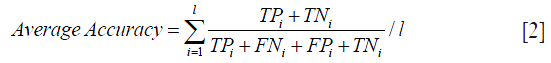
where TP is the true positive, TN is the true negative, FP is the false positive and FN is the false negative. The subscript i indicates category, and l refers to the total category.

The CrossTable() function returns the result of cross tabulation of predicted and observed classifications. The number in each cell can be used for the calculation of four basic parameters true positive (TP), true negative (TN), false negative (FN) and false positive (FP). The process repeated for each category. Finally, the accuracy is 0.93.

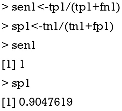
Sensitivity and specificity

Sensitivity is a measure of the proportion of positives that are correctly identify positive observations. Specificity is a measure of the proportion of negatives that are truly negative. They are commonly used to measure the diagnostic performance of a test (9). In evaluation of a prediction model, they can be used to reflect the performance of the model. Imaging a perfectly fitted model that can predict outcomes with 100% accuracy, both sensitivity and specificity are 100%. In multiclass situation as in our example, sensitivity and specificity are calculated separately for each class. The equations are as follows.

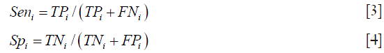
where TP is the true positive, TN is the true negative, FP is the false positive and FN is the false negative. The subscript i indicates category.

Multiclass area under the curve (AUC)

A receiver operating characteristic (ROC) curve measures the performance of a classifier to correctly identify positives and negatives. The AUC ranges between 0.5 and 1. An AUC of 0.5 indicates a random classifier that it has no value. Multiclass AUC is well describe by Hand and coworkers (10). The multiclass.roc() function in pROC package is able to do the task.

As you can see from the output of the command, the multi-class AUC is 0.9212.

Kappa statistic

Kappa statistic is a measurement of the agreement for categorical items (11). Its typical use is in assessment of the inter-rater agreement. Here kappa can be used to assess the performance of kNN algorithm. Kappa can be formally expressed by the following equation:

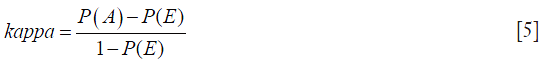
where P(A) is the relative observed agreement among raters, and P(E) is the proportion of agreement expected between the classifier and the ground truth by chance. In our example the tabulation of predicted and observed classes are as follows:

The relative observed agreement can be calculated as

the kNN algorithm predicts 1, 2 and 3 for 31, 7, and 12 times. Thus, the probability that kNN says for 1, 2 and 3 are 0.62, 0.14 and 0.24, respectively. Similarly, the probabilities that 1, 2 and 3 are observed are 0.58, 0.2 and 0.22, respectively. Then, the probability that both classifier say 1, 2 and 3 are 0.62×0.58=0.3596, 0.14×0.2=0.028 and 0.24×0.22=0.0528. The overall probability of random agreement is:

and the kappa statistic is:

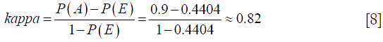
Fortunately, the calculation can be performed by cohen.kappa() function in the psych package. I present the calculation process here for readers to better understand the concept of kappa.

Tuning k for kNN

The parameter k is important in kNN algorithm. In the last section I would like to tune k values and examine the change of the diagnostic accuracy of the kNN model. Custom-made R function is helpful in simplify the calculation process. Here I write a function named “accuracyCal” to calculate a series of average accuracies. There is only one argument for the function. That is the maximum number of k you would like to examine. There is for loop with in the function that calculates accuracy repeatedly from one to N. When you run the function, the results may not exactly the same for each time. That is because the knn() function breaks ties at random. To explain, if we have 4 nearest neighbors and two are classified as A and 2 are classified as B, then A and B are randomly chosen as predicted result.

The following code creates a visual display of the results. An inset plot is created to better visualize how accuracy changes within the k range between 5 and 20. The subplot() function contained in TeachingDemos package is helpful in drawing such an inset. It is interesting to adjust graph parameters to make the figure a better appearance (Figure 3). The figure shows that the average accuracy is highest at k=15. At a large k value (150 for example), all observations in the training dataset are included and all observations in the test dataset are assigned to the class with the largest number of subjects in the training dataset. This is of course not the result we want.

Figure 3 Graphical presentation of average accuracy with different k values. The inset zooms in at k range between 0 and 30.

Summary

The article introduces some basic ideas underlying the kNN algorithm. The dataset should be prepared before running the knn() function in R. After prediction of outcome with kNN algorithm, the diagnostic performance of the model should be checked. Average accuracy is the most widely used statistic to reflect the performance kNN algorithm. Factors such as k value, distance calculation and choice of appropriate predictors all have significant impact on the model performance.

Acknowledgements

None.

Footnote

Conflicts of Interest: The author has no conflicts of interest to declare.

References

1. Short RD, Fukunaga K. The optimal distance measure for nearest neighbor classification. IEEE Transactions on Information Theory 1981;27:622-7. [Crossref]
2. Weinberger KQ, Saul LK. Distance metric learning for large margin nearest neighbor classification. The Journal of Machine Learning Research 2009;10:207-44.
3. Cost S, Salzberg S. A weighted nearest neighbor algorithm for learning with symbolic features. Machine Learning 1993;10:57-78. [Crossref]
4. Breiman L. Random forests. Machine Learning. 2001;45:5-32. [Crossref]
5. Zhang Z. Too much covariates in a multivariable model may cause the problem of overfitting. J Thorac Dis 2014;6:E196-7. [PubMed]
6. Lantz B. Machine learning with R. 2nd ed. Birmingham: Packt Publishing; 2015:1.
7. Venables WN, Ripley BD. Modern applied statistics with S-PLUS. 3rd ed. New York: Springer; 2001.
8. Hernandez-Torruco J, Canul-Reich J, Frausto-Solis J, et al. Towards a predictive model for Guillain-Barré syndrome. Conf Proc IEEE Eng Med Biol Soc 2015;2015:7234-7.
9. Linden A. Measuring diagnostic and predictive accuracy in disease management: an introduction to receiver operating characteristic (ROC) analysis. J Eval Clin Pract 2006;12:132-9. [Crossref] [PubMed]
10. Hand DJ, Till RJ. A simple generalisation of the area under the ROC curve for multiple class classification problems. Machine Learning 2001;45:171-86. [Crossref]
11. Thompson JR. Estimating equations for kappa statistics. Stat Med 2001;20:2895-906. [Crossref] [PubMed]