
Using the confidence interval confidently
Introduction
Biomedical research is seldom done with entire populations but rather with samples drawn from a population. There are various strategies for sampling, but, wherever feasible, random sampling strategies are to be preferred since they ensure that every member of the population has an equal and fair chance of being selected for the study. Random sampling also allows methods based on probability theory to be applied to the data.
Although we work with samples, our goal is to describe and draw inferences regarding the underlying population. Values obtained from samples are referred to as ‘sample statistics’ which we have to use to garner idea of corresponding values in the underlying population, that are referred to as ‘population parameters’. But how do we do this? If we are doing ‘census’ type of studies, then the measured values are directly the population parameters since a census covers the entire population. However, if we are studying samples, then what we have in our hand at study end are the sample statistics. If we have a large enough and adequately representative sample, it is logical to presume that the sample statistics would be close to the ‘true values’, that is the population parameters, but they would probably not be identical to them. Strictly speaking, without doing a census it is not possible to get true population values. Practically speaking, it is possible to use a sample statistic and estimates of error in the sample to get a fair idea of the population parameter, not as a single value, but as a range of values. This range is the confidence interval (CI). How well the sample statistic estimates the underlying population value is always an issue. The CI addresses this issue because it provides a range of values which is likely to contain the population parameter of interest.
The CI is a descriptive statistics measure, but we can use it to draw inferences regarding the underlying population (1). In particular, they often offer a more dependable alternative to conclusions based on the P value (2). They also indicate the precision or reliability of our observations—the narrower the CI of a sample statistic, the more reliable is our estimation of the underlying population parameter. Wherever sampling is involved, we can calculate CI. Thus we can calculate CI of means, medians, proportions, odds ratios (ORs), relative risks, numbers needed to treat, and so on. The concept of the CI was introduced by Jerzy Neyman in a paper published in 1937 (3). It has now gained wide acceptance although many of us are not quite confident about it (4). To be fair it is not an intuitive concept but requires some reflection and effort to understand, calculate and interpret correctly. In this article we will look at these issues.
Meaning of CI
The CI of a statistic may be regarded as a range of values, calculated from sample observations, that is likely to contain the true population value with some degree of uncertainty.
Although the CI provides an estimate of the unknown population parameter, the interval computed from a particular sample does not necessarily include the true value of the parameter. Therefore, CIs are constructed at a confidence level, say 95%, selected by the user. This implies that were the estimation process to be repeated over and over with random samples from the same population, then 95% of the calculated intervals would be expected to contain the true value. Note that the stated confidence level is selected by the user and is not dependent on the characteristics of the sample. Although the 95% CI is by far the most commonly used, it is possible to calculate the CI at any given level of confidence, such as 90% or 99%. The two ends of the CI are called limits or bounds.
CIs can be one or two-sided. A two-sided CI brackets the population parameter from both below (lower bound) and above (upper bound). A one-sided CI provides a boundary for the population parameter either from above or below and thus furnishes either an upper or a lower limit to its magnitude.
Calculation of CIs
Formulas for calculating CIs take the general form:
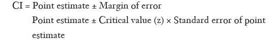
The point estimate refers to the statistic calculated from sample data. The critical value or z value depends on the confidence level and is derived from the mathematics of the standard normal curve. For confidence levels of 90%, 95% and 99% the z value is 1.65, 1.96 and 2.58, respectively. The standard error depends on the sample size and the dispersion in the variable of interest.
Calculation of the CI of the mean is relatively simple. Here the formula is:
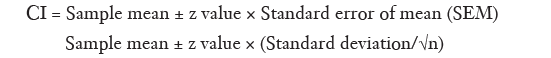
If we are calculating the 95% CI of the mean, the z value to be used would be 1.96. Table 1 provides a listing of z values for various confidence levels. The margin of error depends on the size and variability of the sample. Naturally, the error will be smaller if the sample size (n) is large or the variability of the data [standard deviation (SD)] is less and this is reflected in the SEM.

Full table
Ideally the SD used in the calculation should be the population SD. However, this is often unknown and if we are dealing with a reasonably large (say n >100, or at least >30) random sample, then the sample SD can be used as a fair approximation of the population SD. If the sample is small and one has to rely on the sample SD, then this requires derivation of the CI using the t distribution rather than the z value from the normal distribution. In this situation, the z value is to be replaced with the appropriate critical value of the t distribution with (n–1) degrees of freedom. Note that the Student’s t distribution, resembles the normal distribution, although its precise shape depends on the sample size. The required t value can be found from a t distribution table included in most statistical textbooks. For example, if the sample size is 25, the critical value for the t distribution that corresponds to a 95% confidence level with 24 degrees of freedom, is 2.064.
Let us now work out an example. The mean systolic blood pressure (SBP) and diastolic blood pressure (DBP) of 72 randomly selected chest physicians aged over 50 is 134 and 88 mmHg, with SD of 5.2 and 4.5 mmHg. What is the 95% CIs for the blood pressure readings?
Here we will consider the sample SD as fair approximation to the population SD. Therefore:

Thus the chest physicians appear to be non-hypertensive at present although they still need to keep a regular check on their blood pressure readings.
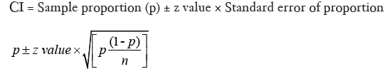
Unlike numerical variables, categorical variables are summarized as counts or proportions, and we will now deal with CI of a proportion. The formula for this is a bit more intimidating, but is still manageable for manual calculation.
Let us work through an example. A radiology resident has done a small observational study to find out the sensitivity and specificity of pleural effusion detected on digital chest X-rays (CXR) in predicting the risk of malignancy among subjects presenting with suggestive clinical findings. Her data is summarized in Table 2.

Full table
The sensitivity of his diagnostic modality is [63/(63+25)]×100, i.e., 71.59%, while specificity is [53/(33+53)]×100, i.e., 61.63%; The 95% CI for the sensitivity would be:

And the 95% CI for the specificity would be:

In this same example, the odds of malignancy being present when pleural effusion is detected on CXR is 63/33, i.e., 1.9091, while the odds when pleural effusion is absent is 25/53, i.e., 0.4717. Therefore the OR for detecting malignancy when pleural effusion is present, compared to when it is absent, would be 1.9091/0.4717, i.e., 4.047.
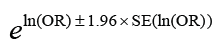
Calculation of the 95% CI of the OR requires a more complicated formula, where we first derive the natural logarithm (log to base e, or ln) of the sample OR and then calculate its standard error. From this we derive the two confidence limits of the ln(OR), and then take their antilog to derive the 95% CI of the OR.
The formula is:
Where, 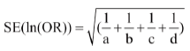
Thus in the above example ln(OR) would be
The SE of ln(OR) would be 1.3980±1.96×0.3241=1.3980±0.6352, i.e., 0.7628 to 2.0332.
The 95% confidence limits for ln(OR) would be
Taking antilog of these two boundaries, the 95% CI of OR of 4.047 in this case would be 2.144 to 7.638. Note that since this 95% CI of the OR does not span the value 1, it implies that a pleural effusion detected by CXR in a patient with clinical examination findings suggestive of malignancy is approximately 2.1 to 7.6 times as likely to indicate malignancy than when it is not detected.
The reason why we resort to such an apparently complicated formula is that ORs are not normally distributed. They tend to be skewed towards the lower end of possible values. As a result, we must take the natural log of the OR and first compute the confidence limits on a logarithmic scale, and then convert them back to the normal OR scale. The same applies to relative risks and other sample statistics that are skewed in this manner.
Calculating CIs for distribution free statistics
From the examples above, it should be evident that CI take the general form of Point estimate ± Margin of error, where the margin of error is calculated by multiplying a critical value selected as per the required confidence limits with the standard error.
Standard errors cannot be calculated for distribution free statistics. Nevertheless, CIs can be calculated and have the same interpretation, that is they will present a range of values with which the true population value is compatible. In this case, the confidence limits are not necessarily symmetric around the sample estimate and are given by actual values in the sample that are chosen from the applicable formula.
The formula for calculating the CI of the median is:
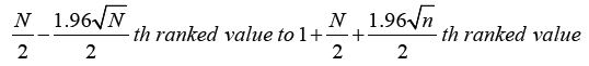
For example, if there are 100 values in a sample data set, the median will lie between 50th and 51st values when arranged in ascending order. Applying the formula shown above, the lower 95% confidence limit is indicated by 40.2 rank ordered value, while the upper 95% confidence limit is indicated by 60.8 rank ordered value. Since there are no actual 40.2 and 60.8 ranked values, we choose the ranks nearest to these and values of these ranks then provide the approximate 95% CI for the median. For the 100 value series, this will therefore be the range indicated by the 40th to 61st rank ordered value.
For large samples, the CI for the median and other quartiles can be determined on the basis of the binomial distribution. You can see examples online (5).
Factors affecting the width of the CI
The width of the CI indicates the utility of our estimation of the population parameter. Suppose the weather forecaster uses the concept of the 99% CI to declare that tomorrows maximum temperature is going to be anywhere between 1 to 50 °C. It is extremely unlikely that he or she will be wrong but for you and me it would be utmost perplexing as to what to wear outdoors tomorrow. On the other hand if he says that the range is likely to be 20 °C to 30 °C on the basis of the 95% CI, then he has more chance of being wrong but it is easier for us to decide how we dress tomorrow. The factors affecting the width of the CI include the desired confidence level, the sample size and the variability in the sample.
The width of the CI varies directly with the confidence level. A 99% CI would be wider than the corresponding 95% CI from the same sample. This stands to reason, since a larger likelihood of containing the true population value would lie with the wider interval.
A larger sample size expectedly will lead to a better estimate of the population parameter and this is reflected in a narrower CI. The width of the CI is thus inversely related to the sample size. In fact, required sample size calculation for some statistical procedures is based on the acceptable width of the CI.
Variability in a random sample directly influences the width of the CI. A larger spread implies that it is more difficult to reliably estimate population value without large amounts of data. Thus as the variability in the data (often expressed as the SD) increases, the CI also widens.
Practical use of the CI
In descriptive statistics, CIs reported along with point estimates of the variables concerned, indicate the reliability of the estimates. The 95% confidence level is often used, though the 99% CI are used occasionally. At 99%, the width of the CI will be larger but it is more likely to contain the true population value, than the narrower 95% CI. Bioequivalence testing makes use of the 90% CI. In such studies, we can conclude that two formulations of the same drug are not different from one another if the 90% CI of the ratios for peak plasma concentration (Cmax) and area under the plasma concentration time curve (AUC) of the two preparations (test vs. reference) lies in the range 80–125%.
Conflict between clinical importance and statistical significance is an important issue in biomedical research. Clinical importance is best inferred by looking at the effect size, that is how much is the actual change or difference. However, statistical significance in terms of P only suggests whether there is any difference in probability terms (6). One way to combine statistical significance and effect sizes is to report CIs. If a corresponding hypothesis test is performed, the confidence level is the complement of the level of significance, that is a 95% CI reflects a significance level of 0.05, while at the same time providing an estimate of the ‘true’ value. Indeed, if there is no overlap on comparing 95% CI surrounding point estimates of the outcome variable in different groups, once can conclude that statistically significant difference exists. On the other hand, even if there is small overlap, the difference between groups may not be clinically significant, irrespective of the P value. Thus stating the CI shifts the interpretation from a qualitative judgment about the role of chance to a quantitative estimation of the biologic measure of effect (7).
Of late, clinical trials are being designed specifically as superiority, non-inferiority or equivalence studies. The conclusions from these alternative trial designs are based on CI values rather than the P value from intergroup comparison (8). CI around the outcome point estimate for the test drug must fall wholly within a predefined equivalence margin on both sides of the line of no difference for establishing equivalence. For establishing non-inferiority, the lower bound of the 95% CI for the test drug must not cross the non-inferiority margin set a priori. For establishing superiority, the lower bound of the 95% CI for the test drug must lie beyond the line of no difference, while the upper bound extends beyond the superiority margin set a priori. Figure 1 summarizes these situations graphically. Selection of these margins has to be done with due care based on clinical judgment.

The concept of CIs and confidence levels are also used in the calculation of sample size for prevalence surveys. The margin of error selected by the surveyor determines the acceptable deviation between the prevalence in the surveyed section of the population and the prevalence in the entire population. Thus, the margin of error implies a CI. The confidence level selected indicates how often the percentage of the population that has the condition of interest is likely to lie within the boundaries decided by the margin of error. Table 3 indicates how required sample size for population surveys varies with acceptable margin of error and confidence level.

Full table
Misconceptions regarding the CI
A 95% CI does not mean that 95% of the sample data lie within that interval. A CI is not a range of plausible values for the sample, rather it is an interval estimate of plausible values for the population parameter.
It is natural to interpret a 95% CI as a range of values with 95% probability of containing the population parameter. However, the proper interpretation is not that simple. The true value of the population parameter is fixed, while the width of the 95% CI based on a random sample will also vary randomly. If we take repeated random samples of equal size from the population, we will get a corresponding number of 95% CI values not all of which will contain the population parameter—in fact only 95% of them can be expected to contain the population parameter value. Thus the CI may not always give an idea of the population parameter.
Selection of the acceptable confidence level is arbitrary. We often use the 95% CI in biological sciences, but this is a matter of convention. A much higher level is often used in the physical sciences. For instance the six sigma concept, the quality improvement program that Motorola originated, and which is now popular in many manufacturing companies, utilizes a confidence level of 99.99966% (9). The engineers want to eliminate all risk of manufacturing poor-quality products and therefore work at this level of precision.
Finally, it is worthwhile to remember that the concept of the CI was introduced to provide an answer to the vexing issue in statistical inference of how to deal with the uncertainty inherent in results derived from data that represent randomly selected subset of a population. There are other answers, notably that provided by Bayesian inference in the form of credible intervals. Calculation of the conventional CI depends on set rules that ensure that the interval determined by the rule will include the true value of the population parameter. This is the so called ‘frequentist’ approach. The Bayesian approach offers intervals that can, subject to acceptance of interpretation of ‘probability’ as Bayesian probability, be interpreted as meaning that the specific interval calculated from a given dataset has a particular probability of including the true value, conditional on the particular situation (10). Bayesian intervals treat their bounds as fixed and the estimated parameter as a random variable, whereas conventional approach treats confidence limits as random variables and the population parameter as a fixed value. Unlike the Bayesian method, the frequentist method of computing CIs does not make use of any other prior information regarding the location of the population parameter. Thus, there is a philosophical difference between the two approaches which we can address at a later stage.
Acknowledgements
None.
Footnote
Conflicts of Interest: The author has no conflicts of interest to declare.
References
- Altman DG. Why we need confidence intervals. World J Surg 2005;29:554-6. [Crossref] [PubMed]
- Akobeng AK. Confidence intervals and p-values in clinical decision making. Acta Paediatr 2008;97:1004-7. [Crossref] [PubMed]
- Neyman J. Outline of a theory of statistical estimation based on the classical theory of probability. Philos Trans R Soc Lond A 1937;236:333-80. [Crossref]
- Hoekstra R, Morey RD, Rouder JN, et al. Robust misinterpretation of confidence intervals. Psychon Bull Rev 2014;21:1157-64. [Crossref] [PubMed]
- Bland M. Confidence interval for a median and other quantiles [Monograph on the internet]. Available online: https://www-users.york.ac.uk/~mb55/intro/cicent.htm
- Thiese MS, Ronna B, Ott U. P value interpretations and considerations. J Thorac Dis 2016;8:E928-31. [Crossref] [PubMed]
- Medina LS, Zurakowski D. Measurement variability and confidence intervals in medicine: why should radiologists care? Radiology 2003;226:297-301. [Crossref] [PubMed]
- Lesaffre E. Superiority, equivalence, and non-inferiority trials. Bull NYU Hosp Jt Dis 2008;66:150-4. [PubMed]
- Anonymous. What is a confidence interval and why would you want one? [Monograph on the internet]. Available online: http://www.uxmatters.com/mt/archives/2011/11/what-is-a-confidence-interval-and-why-would-you-want-one.php
- Jaynes ET. Confidence intervals vs Bayesian intervals. In: Harper WL, Hooker CA, editors. Foundations of probability theory, statistical inference, and statistical theories of science. Vol II. Dordrecht: D. Reidel Publishing Company 1976:175-257.

