A comparison of association methods for cytotoxicity mapping in pharmacogenomics

Cytotoxicity assays of immortalized lymphoblastoid cell lines (LCLs) represent a promising new in vitro approach in pharmacogenomics research. However, previous studies employing LCLs in gene mapping have used simple association methods, which may not adequately capture the true differences in non-linear response profiles between genotypes. Two common approaches summarize each dose-response curve with either the IC50 or the slope parameter estimates from a hill slope fit and treat these estimates as the response in a linear model. The current study investigates these two methods, as well as four novel methods, and compares their power to detect differences between the response profiles of genotypes under a variety of different alternatives. The four novel methods include two methods that summarize each dose-response by its area under the curve, one method based off of an analysis of variance (ANOVA) design, and one method that compares hill slope fits for all individuals of each genotype. The power of each method was found to depend not only on the choice of alternative, but also on the choice for the set of dosages used in cytotoxicity measurements. The ANOVA-based method was found to be the most robust across alternatives and dosage sets for power in detecting differences between genotypes.

1. Introduction

Important progress continues to be made in the treatment of most common cancers, but therapeutic benefit remains difficult to predict and severe or fatal adverse events occur frequently. The Human Genome Project has fueled the notion that genetic information can produce effective and cost-efficient selection of therapies for individual patients (Manolio et al., 2008), but validated genetic signatures that predict response to most chemotherapy regimens have yet to be identified. Numerous genes potentially influence drug response, but current candidate-gene approaches aimed at discovering and characterizing pharmacogenetic effects are limited by the requirement of a priori knowledge about the genes involved (Auman and McLeod, 2008). While genome-wide association analyses represent unbiased approaches to trait mapping, the moderate size of most clinical trials often limits this avenue for cancer pharmacogenomics discovery (Ratain et al., 2006). Furthermore, many pharmacogenomic studies are performed with the unstated and untested assumption that the drug response is a heritable trait, potentially wasting scarce clinical and analytical resources if this assumption proves false.

In response to these limitations, a novel in vitro assay system has emerged as a promising new approach for gene mapping in pharmacogenomics cancer therapy (Watters et al., 2004). This in vitro system relies on cytotoxicity assays of immortalized lymphoblastoid cell lines (LCLs) to measure dose-response phenotypes of individual cell lines (Dolan et al., 2004; Watters et al., 2004; Huang et al., 2007; Bleibel et al., 2009; Duan et al., 2009; Peters et al., 2009, 2011a; Gamazon et al., 2010; Stark et al., 2010; Watson et al., 2011a,b). While the direct translational relevance of these assays is not fully understood, LCL-based assay systems can be used to measure interindividual response to cytotoxic drugs, and to assess and map the genetic components that explain this variability (Zhang et al., 2008; Welsh et al., 2009). Unlike the practical limitations of in vivo pharmacogenomic mapping, mentioned above, family-based and population-based cohorts can be assayed to perform heritability assessment (Stark et al., 2010; Peters et al., 2011a; Watson et al., 2011b), linkage mapping (Peters et al., 2011a; Watson et al., 2011a,b), and association mapping (Huang et al., 2011).

While initial studies are exciting, there are many statistical and computational challenges presented by such data, especially when fine-mapping with genome-wide genotyping approaches are considered. The large-scale of such in vitro studies presents interesting and important analytical, computational, and statistical challenges. This model system generates high-throughput data at several biological levels. The drug response outcomes are measured for a large number of drugs, for many dose points, and for a large number of cell lines and replicates. There are several potential sources of noise in this phenotype collection that need to be considered in analysis. Summarizing response across doses requires non-linear modeling, and traditional methods may not be suitable for high-throughput data (Beam and Motsinger-Reif, 2010). Additionally, there are important open questions in how best to test for associations of the genetic data (genome-wide association data with millions of single nucleotide polymorphisms, SNPs) with these non-linear dose-response outcomes.

Previous studies that have performed gene mapping have employed simple association methods, using summary measures from non-linear modeling of the dose-response curves (Dolan et al., 2004; Watters et al., 2004; Huang et al., 2007; Bleibel et al., 2009; Duan et al., 2009; Peters et al., 2009, 2011a; Gamazon et al., 2010; Stark et al., 2010; Watson et al., 2011a,b). These studies have summarized dose-response with either IC50 values (the interpolated dose at which 50% of cells have been killed), or the hill slope (the slope of the non-linear model) estimated for each individual (Beam and Motsinger-Reif, 2010). While this approach is seemingly straightforward, there are both biological and statistical assumptions that are propogated in this analysis strategy. Such analyses assume that differential response is defined by one parameter of a complex non-linear model (discussed more below), which may not capture the true array of potential differential response. This assumption will limit the power of such approaches to detect other types of differential response (if the assumption is not correct), and may introduce error into the association analysis by assuming a summary measure captures all information about the dose-response curve. There are well-documented challenges in non-linear dose-response modeling, that are of particular concern in high-throughput studies (Beam and Motsinger-Reif, 2010).

In order for such in vitro assays to reach their full potential for gene mapping, proper analytical strategies need to be tested and developed to take full advantage of this complex data. In the current study, we perform a large-scale simulation study to compare and contrast analytical approaches for association analysis. We compare the two approaches previously reported, and propose and evaluate new approaches that use the dose-response curves. We use real cytotoxicity data from dose-response data of Gemcitabine to motivate realistic data simulation, and simulate a wide range of genetic association models to evaluate these methods. Methods are evaluated based on power, computational simplicity, and robustness and minimization of model assumptions. We hope that these results will guide the proper application of powerful association methods to detect genetic associations in in vitro cytotoxicity data.

2. Materials and Methods

2.1. Use of Real Data to Guide Simulation Study

A major challenge of many simulation studies is the generation of data that are representative of real data and are likely to be encountered in practice. This is especially true for cell line data, where dose-response curves are necessarily non-linear and the distribution of error terms may not be normal, as explained below. In addition, the non-linear effects between viability and drug concentration can be different for every cell line.

For this reason, simulated data was modeled after real data from 264 LCLs exposed to the cancer drug Gemcitabine. See Section A1 in Appendix for experimental details. Each cell line was exposed to six different concentrations of the drug, with four replications at each concentration. The concentrations (in mM) used were: 1.0 × 10⁻⁴, 4.0 × 10⁻⁵, 2.0 × 10⁻⁵, 8.0 × 10⁻⁶, 5.0 × 10⁻⁶, and 2.5 × 10⁻⁶. This drug produced responses that generally had a smooth sigmoidal shape.

Several quality control (QC) measures were used to maximize the integrity of the real data. The dose-response data for two cell lines were eliminated because of poor viability. Two other cell lines had 10% dimethyl sulfoxide viability readings that were too high to be realistic (possibly due to the chemical adhering to the side of the plate well). These high readings were exchanged for the same measurements with the same cell lines from another experiment. In addition, whenever the coefficient of variation (CV) for a block of four replications exceeded 0.4796, the most deviant response was replaced with the mean of the other three. This step was repeated, if necessary. This resulted in 0.2% of the responses being replaced.

Briefly, these parameters were chosen based on parameter sweeps across a large number of drug response experiments (Motsinger-Reif et al., 2011; Peters et al., 2011b). The QC approach was aimed to reduce noise and outliers in the data, while still preserving meaningful variation in the data. The CV cutoffs were chosen based on the distribution of CV seen across the data for hundreds of cell lines across twenty eight drugs, using the 99th percentile to determine the cutoff value. In our experience, such a high CV could generally be traced back to a single extremely errant value (orders of magnitude away from the others), and we feel represents technical error and not true variation.

After preliminary QC, responses were normalized according to the equation:

where Y_ijk,Raw is the raw data response for a sample from the ith cell line exposed to the jth drug concentration for the kth replication and Y_ijk is the normalized response. Also, is the average response of four readings of the same cell line exposed to a 10% dimethyl sulfoxide solution (thought to kill all living cells), and is the average of four readings of the same cell line exposed to a 0.1% dimethyl sulfoxide solution. This latter solution was the vehicle used for all experiments, and was needed to solvate the drug.

After this normalization, a final QC measure replaced deviant responses (similar to that above) using a CV threshold of 0.25. This resulted in an additional 0.6% of responses being replaced. After imputation of deviant responses and normalization, many responses still exceeded their expected maximum of one. Therefore, the responses for each cell line were individually scaled, if necessary, so that the mean response of the lowest concentration was no greater than 1.0. This resulted in 63% of response curves being scaled.

Cell line responses from Gemcitabine were used to estimate parameter distributions and residual distributions for the simulated data. Each individual curve was assumed to follow a hill slope function, and parameter estimates were made for each individual. The distribution of individual curves was then modeled by estimating the distributions of these (estimated) hill slope parameters. The hill slope equation used was used to fit dose-response curves:

where x_j is the concentration of drug that response Y_ijk was exposed to. All of the β_i parameters have biological interpretation. The parameter represents the expected response as concentration, x_j, approaches zero, while the parameter represents the expected response as concentration, x_j, approaches infinity. The parameter reflects that concentration which gives a response halfway between and The parameter has the interpretation of being proportional to the slope of the tangent line when concentration Stated otherwise, a very negative will cause a sharp drop in response when the concentration is near The β⁽²⁾ and β⁽³⁾ parameters are frequently referred to as the “IC50” and “Slope” parameters in the literature. We will refer to β⁽⁰⁾ and β⁽¹⁾ as the “Max” and “Min” parameters, respectively.

The curve-fitting algorithm, described in Section A2 in Appendix, was used to fit hill slope curves to all 262 cell lines from the Gemcitabine data. Generally, the fits were very good, as indicated in a plot of fitted dose-response curves from nine random cell lines in Figure 1.

FIGURE 1

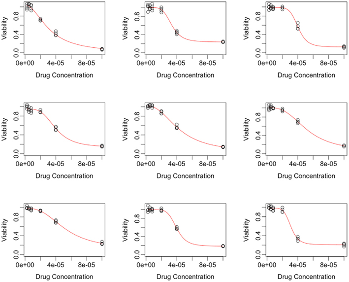
Figure 1. Hill slope functions fit to real data from nine random Gemcitabine dose-response curves.

The distributions for each of the hill slope parameters were modeled as either gamma or Laplace. The goal was not to reproduce the distribution of the hill slope parameters exactly, but to get a sense of what the distribution for these parameters would be for a typical cancer drug. Distributional parameters for each hill slope parameter were then estimated using maximum likelihood via R’s “nlm” routine (R Development Core Team, 2010). Figure 2 shows histograms of the hill slope parameters with the fitted distributions overlaid. The histograms are of the estimated hillslope parameters from the 262 viable cell lines exposed to Gemcitabine, while the fitted distributions were used for generating realizations of hillslope parameters as part of the simulation. In a similar manner, the distribution of residuals were modeled as Laplace. The distributions for the hill slope parameters and residuals were used together for the generation of simulated data, as explained in Section 2.2.

FIGURE 2

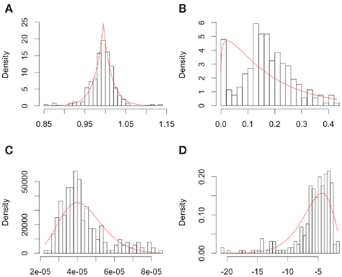
Figure 2. Plots of individual hill slope parameters for Gemcitabine. Histograms represent parameters estimated from observed real data, while red lines represent the distribution for parameters used in simulation. (A–D) represent the distributions for the Max, Min, IC50, and slope parameters, respectively.

2.2. Data Simulation

Data was simulated in sets of 496 dose-response curves. For each null distribution, 10,000 data sets were generated, while 2500 data sets were generated for each alternative. Each data set is characterized by its genetic model, minor allele frequency (MAF), affected parameter, effect size, and set of drug concentration values. Each dose-response curve contained twenty-four dose-response pairs, comprised of four replications at each of six concentrations. Genotype frequencies were calculated according to MAF using Hardy-Weinberg Equilibrium (Hardy, 1908; Weinberg, 1908). The distributional means for the affected parameters were modified according to the cell line’s genotype and the data sets’ genetic model and effect size (the distributional variances remained constant throughout), as explained in the following paragraphs.

Let A and a represent the major and minor alleles, respectively. For the additive model, the mean of the affected parameter was made more extreme by the effect size for genotype Aa and by twice the effect size for genotype aa. For the dominant model, the mean of the affected parameter was made more extreme by twice the effect size for genotype aa, only. A dose-response curve was constructed by first generating hill slope parameters, according to their estimated distributions and effect size modifications. Responses were then simulated by calculating the mean response at each drug concentration (using the hill slope function), and adding residual noise. The estimation procedure of the distributions for parameters and residuals are described in Section 2.1.

This process is illustrated below under the null, where Y_ijkl is the response for the lth replication at drug concentration x_k for the jth cell line having the genotype i:

where f(x_k,β_ij) is the hill slope function given in Eq. 1. Although parameters were generated independently of each other, a check was added to the simulation that ensured that If a simulated β_ij value failed this check, the parameter vector was discarded and regenerated (this occurred with probability 0.003). This check guaranteed that dose-response curves decreased in viability as drug concentration increased, and ensured that extreme outliers for estimates of were avoided.

Under the alternative, if is an affected parameter (p ∈ {1,2,3}), the shape and scale parameters for the gamma distribution of are adjusted such that the mean is increased according to the genotype, effect size and genetic model, and the variance remains unchanged. For example, if K is the effect size, under an additive genetic model, we see that the mean of is adjusted:

where is the mean and is the standard deviation of under the null. Then we have the distribution for :

For data generated under the null distribution, three MAF’s (0.1, 0.25 and 0.5) and two sets of drug concentrations were used in data simulation. The first set uses six concentrations equally spaced over the “action range” of the hill slope equation: (in mM) 3.125 × 10⁻⁶, 2.75 × 10⁻⁵, 5.1875 × 10⁻⁵, 7.625 × 10⁻⁵, 1.00625 × 10⁻⁴, and 1.25 × 10⁻⁴. The second set uses six concentrations equally spaced on the log scale, using the same range as the first set: 3.125 × 10⁻⁶, 6.25 × 10⁻⁶, 1.0 × 10⁻⁵, 2.5 × 10⁻⁵, 5.0 × 10⁻⁵, and 1.25 × 10⁻⁴. This latter set is the same as was used in the real data.

For data generated under the alternative, the affected parameters include β⁽¹⁾, β⁽²⁾, and β⁽³⁾. For each of these parameters and each MAF from above, six effect sizes were used; 0.0, 0.1, 0.2, 0.3, 0.4, and 0.5. The “0.0” effect size actually simulates data under the null distribution, using a different random number starting seed, and is used to estimate the type I error rate. For each affected parameter, MAF and effect size, data was simulated according to either a dominant or additive genetic model. Finally, for each of these combinations, one of the two sets of drug concentrations was used. All of these simulations are described in Table 1.

TABLE 1

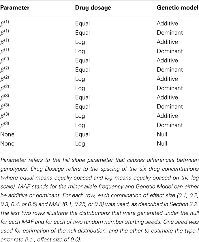
Table 1. Simulations performed in the current study.

2.3. Statistical Methods

Previously, investigators of LCL cytotoxicity data have used two primary methods in searching for meaningful single nucleotide polymorphisms (SNPs; Dolan et al., 2004; Watters et al., 2004; Huang et al., 2007; Bleibel et al., 2009; Duan et al., 2009; Peters et al., 2009, 2011a; Gamazon et al., 2010; Stark et al., 2010; Watson et al., 2011a,b). These two methods summarize the dose-response curve by the IC50 and Slope parameters estimated by the best-fit hill slope curve. Both methods can be considered to fall into the same class of methods (see Section 2.3.1 below). The current study compares the performance of these two methods, along with a new class of methods, with two novel methods from each class, on simulated data.

2.3.1. Univariate and multivariate methods

All methods considered make some use of analysis of variance (ANOVA). One class of methods, univariate methods, makes a univariate summary of each dose-response curve and performs ANOVA against genotype:

where (Y_ij, x_ij) represents the jth dose-response curve for genotype i, α_i represents the fixed effect for genotype i, and s(Y_ij, x_ij) ∈ ℝ. The advantage of these methods is that the error terms are independent, and typical tests of significance using the F-distribution are valid. A disadvantage is the assumption that differential response between genotypes is defined by one parameter of a complex non-linear model. This may not capture the true array of potential differential response and may limit the power of such approaches to detect other types of differential response.

Another class of methods, multivariate methods, attempts to make use of all of the information contained in (Y_ij, x_ij) by comparing a full model, that uses genotype and drug concentration to predict the response, to a reduced model that only uses drug concentration. The full model and reduced models can be characterized by:

In this case, an F-statistic can be calculated:

where SSE_R, SSE_F, df_R, df_F, are the sums of squared errors, and degrees of freedom for the full and reduced models. The disadvantage with this method is that the error terms are correlated within individuals (i.e., Cov[e_ijkl, e_ijk′l′] ≠ 0).

2.3.2. IC50 and slope

The first two methods considered are univariate, and summarize (Y_ij, x_ij) with either the β⁽²⁾ or β⁽³⁾ parameter that is estimated by the best-fit hill slope curve. If the true difference in curves between genotypes is due to differences between β⁽²⁾ or β⁽³⁾ values, and these parameters can be estimated accurately, then these methods can be expected to perform well in detecting differences between genotypes. Here, the ANOVA model is:

where is the estimated β⁽²⁾ or β⁽³⁾ parameter for (Y_ij, x_ij). With a slight abuse of notation, the methods using estimated β⁽²⁾ and β⁽³⁾ parameters will be referred to as the IC50 and Slope methods, respectively. This is not to be confused with alternative distributions created by differences in the IC50 and Slope parameters between genotypes.

2.3.3. Area under the curve

The next two methods are also univariate, and summarize (Y_ij, x_ij) with the area under the dose-response curve (AUC) for some maximum concentration value M and minimum value m:

where f(x, β_ij) is given in Eq. 1. In the current study, M was chosen to be 1.5 times the maximum dose from the dose-response curve (in this case 1.875 × 10⁻⁴), and m was the minimum dose (3.125 × 10⁻⁶). The closed form solution for this integral is complicated, so it was approximated in two ways. First, the integral can be approximated by its Riemann sum:

where

and P is any large integer (P = 20 in the current simulation). Here, is the parametric approximation to AUC_ij. For equally spaced drug concentrations, the integral can also be approximated by the average of the mean of the response for each of the concentrations:

where is the empirical approximation to AUC_ij. In either case, these methods involve substituting either or for s(Y_ij, x_ij) in Eq. 1.

2.3.4. ANOVA and GenoCurve

The third model tests the combined significance of the genotype (G_i) and genotype-concentration interaction effects ((GXC)_ij) in the ANOVA model:

where C_j is the drug concentration and G_i is the genotype for response y_ijkl. Here, test statistics are calculated by comparing the full model above to the reduced model y_ijkl = C_j + e_ijkl. The corresponding F-statistic is:

The last model calculates SSE_F using:

and calculates SSE_R using:

The F-statistic is then:

These last two methods will be referred to as the ANOVA and GenoCurve methods, respectively.

2.4. Permutation Testing

Because the error terms in the multivariate methods are not independent, the constructed F-statistics do not follow the typical F-distribution (see Figure 3). For this reason, these methods would require an estimation of the null distribution in order to calculate p-values under the alternative. In practice, permutation (or some equivalent) testing would be necessary. However, due to the sheer computational time involved with permutation testing within a simulation study, the null distribution was estimated by simply sampling 10,000 test statistics under the null distribution. For consistency, this was done for all six methods, although in practice it would only be necessary for the ANOVA and GenoCurve methods. In this way, p-values for each observed test statistic were estimated by the proportion of test statistics under the appropriate null distribution that were larger than the observed statistic.

FIGURE 3

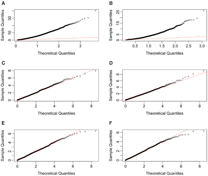
Figure 3. Quantile-quantile plots of test statistics for each method, under H₀ with a MAF of 0.25 and equally spaced drug concentrations. Plots (A–F) represent the methods GenoCurve, ANOVA, IC50, Slope, AUC ^emp, and AUC ^para, respectively. The red dotted line in each plot represents an idealized case where theoretical test statistic quantiles match simulated test statistic quantiles.

2.5. Implementation

All of the analysis was performed using either the R statistical package (R Development Core Team, 2010) or Java. Implementation of all code was performed either on a MacBook Pro (2.66 GHz Intel Core 2 Duo processor with 4 GB 1067 MHz DDR3 memory) or on a computing cluster [two Intel(R) Xeon(R) CPU E5450 processors with 32 GB RAM].

3. Results

Test statistics were generated in two ways for each of the simulation conditions described in Section 2.2. In the first way, hill slope parameters were estimated using the simulated data, while in the second, the true parameter values (generated as part of the simulation) were used for calculating test “statistics.” The quotations reflect that the true parameter values are not a function of the data, and are not typically known in practice. True parameter values were used to calculate the loss in power involved in hill slope parameter estimation. Since only the IC50, Slope, and AUC ^para methods use individual hill slope parameter estimates in calculating test statistics, differences will only be observed for these methods. For each of these methods, scatterplots and correlations of test statistics between estimated and true parameter values are shown in Figure 4 for data generated under the null with a MAF of 0.25. The left hand column of Figure 4 has test statistics calculated using equally spaced drug concentrations, while the right hand column uses concentrations equally spaced on the log scale (see Section 2.2 for details). The correlation between these statistics are strong (0.97, 0.94, and >0.99) for the IC50, Slope, and AUC ^para methods for the equally spaced drug concentrations, but the correlations drop to 0.88 and 0.39 for the IC50 and Slope parameters when the concentrations are equally spaced on the log scale. These results are fairly representative for test statistics drawn from the other alternatives, as well as the null distributions, considered in this study.

FIGURE 4

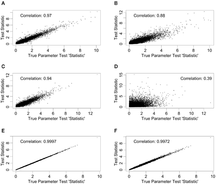
Figure 4. Correlations between test statistics generated using estimated and true parameters. All scatter plots are between test statistics generated under the null hypothesis and a MAF of 0.25. The plots (A,C,E) are of statistics generated from data with equally spaced drug concentrations, while plots (B,D,F) used log-equally spaced data. Plots (A,B) are of the IC50 method, plots (C,D) are of the Slope method, and (E,F) are of the AUC_par method.

There are also correlations for the test statistics between methods (see Figure 5). Here, only the test statistics calculated using estimated parameters are shown, since true parameter values are not typically known in practice. The statistics shown in Figure 5 use the same data (null distribution, with MAF of 0.25) as the ones used in Figure 4, again, with the left hand column representing equally spaced drug concentrations and the right hand column representing drug concentrations equally spaced on the log scale. The most dramatic comparison is between the ANOVA and GenoCurve methods, whose correlation is essentially one for both sets of drug concentration choices. Also the correlations were high between the test statistics for the two AUC methods (0.96 and 0.75 for the two sets of drug concentrations), with more modest correlations between test statistics for the IC50 method and ANOVA methods (0.48 and 0.60 for the two sets of drug concentrations). Again, these results are fairly representative for the other conditions in the study.

FIGURE 5

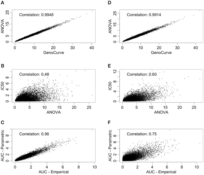
Figure 5. Correlations between test statistics. All scatter plots are between test statistics generated under the null hypothesis and a MAF of 0.25. The plots (A,C,E) are of statistics generated from data with equally spaced drug concentrations, while plots (B,D,F) used log-equally spaced data.

The reason for the higher correlations for the equally spaced vs. the log-equally spaced concentrations is that parameter estimates are more accurate for the former. This makes sense, intuitively, because when the drug concentration sampling scheme is not dense near the “action region,” curves with very different parameter values can still give good fits for the data. However, the total area under the curve tends to be somewhat similar for these different curves. As a dramatic example of this, consider Figure 6, whose data was generated under the null distribution with drug concentrations log-equally spaced. The black and red curves give essentially the same sum of squared errors. However, the percent change from the black curve to the red curve for the Min, IC50, and Slope parameters are (− 111%, 91%, and − 83%), respectively, while percent change for the AUC ^para statistic is only 12% and AUC ^emp is identical for the two curves (since it is estimated using only the data).

FIGURE 6

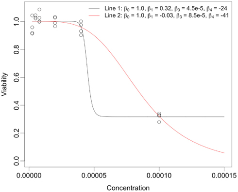
Figure 6. Dramatic example of how very different hill slope curves can give near identical fits for data when drug concentration choices are not well-designed. The legend provides the set of hill slope parameters for each of the lines.

This intuition is substantiated with m-estimation theory. Consider a single dose-response curve {(Y_i, x_i)}, with f (y_i, β) = f_i. Because of least-squares estimation, is an m-estimator:

and E(∂f_i/∂β(Y_i − f_i)) = 0. Therefore:

where

and β_T is the true value for the parameter β. However, β_T varies between cell lines. It follows that:

The first term is the variation in β_T between cell lines, while the second term is the variation due to estimating β_T. From m-estimation theory, we have that (Cox and Hinkley, 1974):

where,

where e_i = Y_i − f_i. Given a value of β_T, these expressions can be evaluated analytically. Therefore generating β_T,i repeatedly from its distribution, calculating , and averaging is a way to approximate E(Σ). This was done for both the equally spaced and log-equally spaced drug concentrations. The percent difference in variance between these concentration choices is given in Table 2. Equal spacing on the log scale gives higher variances than equal spacing for the Min, IC50, and Slope parameters (86, 16, and 10% increases, respectively) and gives a lower variance for the Max parameter (51% decrease).

TABLE 2

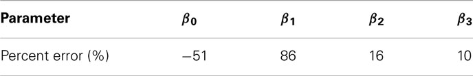
Table 2. Estimated percent change in variation when switching from equally spaced to log-equally spaced drug concentrations.

3.1. Power Comparisons

A p-value was calculated for each test statistic under the alternative, by comparison with its appropriate null distribution as described in Section 2.4. Power was approximated by the proportion of p-values below 0.05. Using STATA (StataCorp, 2011), power was fit as the response in a mixed model analysis, with main effects for genetic model, affected alternative parameter, MAF, dosage, effect size, and method, resulting in a p-value of 0.0299 for the method term.

Power curves for a dominant genetic model, with a minor allele frequency of 0.25, with IC50 as the affected parameter, and with equally spaced drug concentrations, are given in Figure 7A, and also in Table 3. Using an additive genetic model, or increasing the MAF to 0.5 raised powers modestly (results not shown for MAF effects). However, the qualitative implications were the same, with the IC50 method being most powerful, followed by the GenoCurve and ANOVA methods (which had identical power curves), and then by the AUC ^emp and AUC ^para methods. The Slope method never produced power significantly above 0.05 for any method when the affected parameter was IC50. These power curves match well with the power curves produced under the same alternatives using the test statistics derived using true parameter values. This is shown in Figure 7C, with powers being slightly higher for the IC50 method (the ANOVA, and AUC ^emp will be identical, since no hill slope parameters are estimated with these methods). Because p-values were calculated by comparison with an empirically generated null distribution (see Section 2.4 for details), the nominal type I error rate was calculated by comparing test statistics under the null, and using a different random number starting seed, to the same empirically generated null distribution. This resulted in a type I error rate that was within standard error of 0.05 for all methods.

TABLE 3

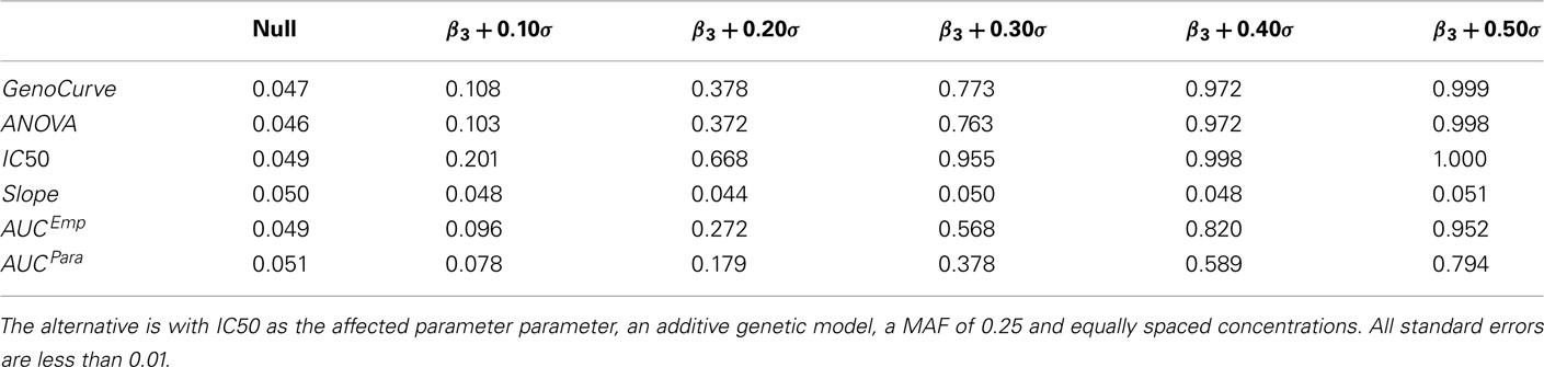
Table 3. Power estimates at α = 0.05 under the alternative using estimated parameters for various effect sizes.

FIGURE 7

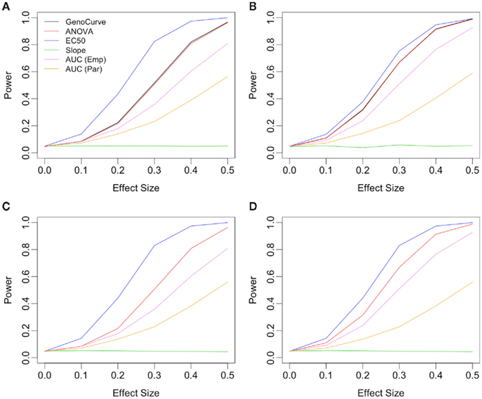
Figure 7. Power plots showing the effects of drug spacing. All plots consider an alternative with IC50 as the affected parameter, with a dominant genetic model and a MAF of 0.25. Plots (A,C) show results for equally spaced drug concentrations, while plots (B,D) show results for log-equally spaced drug concentrations. Plots (C,D) use the true data-generating parameters in calculating test statistics, while in plots (A,B) these parameters are estimated using the data.

The situation is similar for the same alternative using log-equally spaced drug concentrations, as seen in Figure 7. Here, the power for the IC50 method is somewhat lower when using estimated parameters (Figure 7B), than when using the true parameter values (Figure 7D) for the calculation of test statistics. In both cases of drug concentrations, as expected, it appears that when the true differences between genotypes is due to the IC50 parameter, that the IC50 method is most powerful.

When the alternative involves changes to the Slope parameter between genotypes, the power curves are very different. In this case the Slope method uniformly performed best under every alternative as shown in Figure 8C, with ANOVA/GenoCurve as the only other methods ever having power substantially above 0.05. Interestingly, when Min is the affected parameter under the alternative, as shown in Figure 8D, all methods seem to perform similarly except the IC50 and Slope methods, both of which perform poorly. These qualitative results for Min and Slope as the affected parameters remain unchanged under the two genetic models and three MAFs (Figure 8 actually shows results for an additive model with a MAF of 0.5).

FIGURE 8

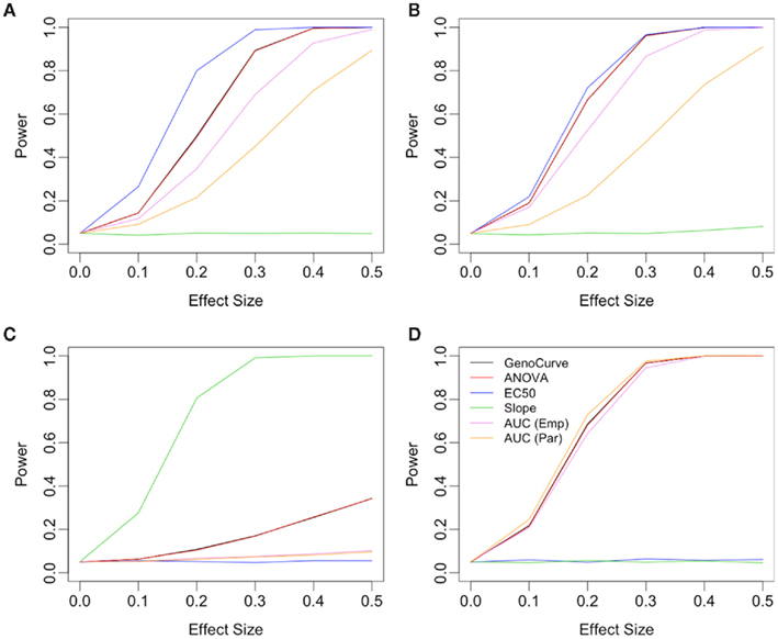
Figure 8. Power plots under various alternatives, effect sizes, and drug concentration spacings. Each plot shows power curves under alternatives with a single affected parameter, with plots (A,B) using the IC50 parameter, plot (C) using the Slope parameter and plot (D) using Min parameter. Plot (B) uses drug concentrations equally spaced on the log scale, while all others are equally spaced. All plots show for an additive genetic model and a MAF of 0.5.

4. Discussion

The current study gave some interesting insight to the performance of various methods used for detecting differences between genotypes for dose-response curves of LCLs. However, there is also a need for improvement in both methods and simulation.

None of the methods considered was especially powerful for all three affected parameters (IC50, Slope, and Min). However, the ANOVA method may be the most robust method for the current choice of alternatives and distribution of hill slope parameters. Although this method was often not the most powerful, it was consistently at least the second most powerful method for every set of alternatives.

The GenoCurve method gave essentially identical power as ANOVA for every alternative. However, the GenoCurve method is computationally less efficient for genome-wide association studies (GWAS). This is because non-linear curve fits must be performed for each genotype, and for each SNP in the GWAS.

The choice for the fixed set of drug concentrations that each LCL is exposed to may be very important for maximizing power to detect differences between genotypes. It is especially important to choose concentrations in the neighborhood of the mean for the population IC50 value, when the true difference between genotypes is IC50. Unsurprisingly, the power of the IC50 method drops when a poor choice of drug concentrations is chosen. When drug concentrations are equally spaced across the expected range of IC50 values from the population, test statistics created from parameters estimated using the data are nearly as powerful as the same “statistics” created with the true parameter values. This indicates that equal spacing may be optimal, or nearly optimal, for this scenario. This result is supported using asymptotic variance arguments.

The current study attempted to simulate data that was similar in spirit to real dose-response data. In this effort, hill slope parameters and residual distributions were estimated from dose-response data from LCLs exposed to the drug Gemcitabine. However, not all of the complexity of the real data was captured in this simulation. For example, the current study assumes that hill slope parameters were independently distributed. However, moderate correlations actually exist, at least between the parameter estimates (see Table 4) in the real data. All of the correlations were significant (with p-values < 0.01), except between β₀ and β₃.

TABLE 4

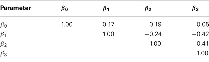
Table 4. Sample Spearman rank correlations between hill slope parameter estimates for dose-response curves of LCLs exposed to Gemcitabine.

However, it is unclear whether the origin of these correlations are due to actual correlations between parameters in the population, or between the estimated parameters from the data. It is possible to have high correlations between estimated parameters, even if the true parameters are not correlated (for example, the slope and intercept estimates are correlated in simple linear regression). This was also demonstrated by generating 1000 random dose-response curves, whose hill slope parameters were generated (independently) according to Section 2.2. For each of these curves, hill slope functions were fit and the resulting hill slope parameters had significant Spearman rank correlations (p-value < 10⁻⁶) between every pair, except β₂ and β₃ (see Table 5).

TABLE 5

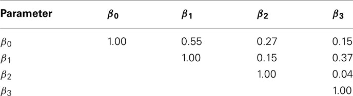
Table 5. Sample Spearman rank correlations between estimates of hill slope parameters for dose-response curves simulated under H₀ with a MAF of 0.25 and equally spaced drug concentrations.

A second limitation is that data was simulated with an assumption of equal variances for error terms among all cell lines. However, in the real data this is not the case, as indicated by highly significant Brown-Forsythe test (p-value <0.0001).In addition, residuals variance was substantially different at different drug concentrations (see Figure 9). Ignoring how variation changes as a function of drug concentration, by using ordinary least-squares (OLS) estimation leads to estimators that are unbiased, but inefficient relative to generalized least-squares (GLS) estimators (Bates and Watts, 1988). It would be interesting to simulate data that captures this pattern of variability, and then compare methods employing OLS estimators to methods using GLS estimators for calculating hill slope parameters.

FIGURE 9

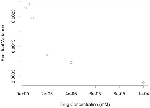
Figure 9. Plots of residual variance vs. concentration for dose-response data of LCLs exposed to Gemcitabine and fit with a hill slope function.

Additionally, the simulations did not take into account measurement error in data, either in the genotyping, or in the concentration levels (Berkson errors). Future studies should evaluate the impact of sure error on the performance of the association analysis methods.

Another interesting method that was not considered is a multivariate ANOVA (MANOVA) approach, where a vector of summary statistics, s(y_ij, x_ij) = {s₁(y_ij, x_ij),…,s_n(y_ij, x_ij)}, is the response (Timm, 2002). This vector could include any combination of the univariate summary statistics considered in this study. This approach attempts to partition the covariance matrix of the response into an effect due to genotype and an effect due to residual error. The partition due to genotype effects can be summarized as a function of its eigenvalues, for example using Wilk’s λ. Because each vector s(y_ij, x_ij) is generated from a single dose-response curve, the vectors are independent and typical F-distributions apply, unlike the ANOVA/GenoCurve methods considered in this study. In addition to multivariate analysis, interactions should also be considered. The current approach only check for univariate genotype effects, but both gene-gene and gene-dose (exposure) effects could be considered. It is reasonable to assume that dose-response outcomes are due to complex genetic etiologies, and future studies should consider interaction effects as one potential genetic architecture.

Conflict of Interest Statement

The authors declare that the research was conducted in the absence of any commercial or financial relationships that could be construed as a potential conflict of interest.

Acknowledgments

This work was supported by Grant Number T32GM081057 from the National Institute of General Medical Sciences and the National Institute of Health.

References

Auman, J. T., and McLeod, H. L. (2008). Cancer pharmacogenomics: DNA genotyping and gene expression profiling to identify molecular determinants of chemosensitivity. Drug Metab. Rev. 40, 303–315.

Pubmed Abstract | Pubmed Full Text | CrossRef Full Text

Bates, D. M., and Watts, D. G. (1988). Nonlinear Regression Analysis and Its Applications. New York, NY: John Wiley and Sons.

Beam, A., and Motsinger-Reif, A. (2010). Optimization of nonlinear dose- and concentration-response models utilizing evolutionary computation. Dose Response 9, 387–409.

Pubmed Abstract | Pubmed Full Text | CrossRef Full Text

Bleibel, W. K., Duan, S., Huang, R. S., Kistner, E. O., Shukla, S. J., Wu, X., Badner, J. A., and Dolan, M. E. (2009). Identification of genomic regions contributing to etoposide-induced cytotoxicity. Hum. Genet. 125, 173–180.

Pubmed Abstract | Pubmed Full Text | CrossRef Full Text

Cox, D. R., and Hinkley, D. V. (1974). Theoretical Statistics. London: Chapman and Hall/CRC.

Dolan, M., Newbold, K., Nagasubramanian, R., Wu, X., Ratain, M., Cook, E., and Badner, J. (2004). Heritability and linkage analysis of sensitivity to cisplatin-induced cytotoxicity. Cancer Res. 64, 4353–4356.

Pubmed Abstract | Pubmed Full Text | CrossRef Full Text

Duan, S., Huang, R. S., Zhang, W., Mi, S., Bleibel, W. K., Kistner, E. O., Cox, N. J., and Dolan, M. E. (2009). Expression and alternative splicing of folate pathway genes in HapMap lymphoblastoid cell lines. Pharmacogenomics 10, 549–563.

Pubmed Abstract | Pubmed Full Text | CrossRef Full Text

Gamazon, E. R., Duan, S., Zhang, W., Huang, R. S., Kistner, E. O., Dolan, M. E., and Cox, N. J. (2010). PACdb: a database for cell-based pharmacogenomics. Pharmacogenet. Genomics 20, 269–273.

Pubmed Abstract | Pubmed Full Text

Hardy, G. (1908). Mendelian proportions in a mixed population. Science 28, 49–50.

Pubmed Abstract | Pubmed Full Text | CrossRef Full Text

Huang, R. S., Duan, S., Bleibel, W. K., Kistner, E. O., Zhang, W., Clark, T. A., Chen, T. X., Schweitzer, A. C., Blume, J. E., Cox, N. J., and Dolan, M. E. (2007). A genome-wide approach to identify genetic variants that contribute to etoposide-induced cytotoxicity. Proc. Natl. Acad. Sci. U.S.A. 104, 9758–9763.

Pubmed Abstract | Pubmed Full Text | CrossRef Full Text

Huang, R. S., Johnatty, S. E., Gamazon, E. R., Im, H. K., Ziliak, D., Duan, S., Zhang, W., Kistner, E. O., Chen, P., Beesley, J., Mi, S., O’Donnell, P., Fraiman, Y. S., Das, S., Cox, N. J., Lu, Y., Macgregor, S., Goode, E. L., Vierkant, R. A., Fridley, B. L., Hogdall, E. V., Kjaer, S. K., Jensen, A., Moysich, K. B., Grasela, M., Odunsi, K. O., Brown, R., Paul, J., Lambrechts, D., Despierre, E., Vergote, I., Gross, J., Karlan, B. Y., Defazio, A., Chenevix-Trench, G., and Dolan, M. E. (2011). Platinum sensitivity-related germline polymorphism discovered via a cell-based approach and analysis of its association with outcome in ovarian cancer patients. Clin. Cancer Res. 17, 5490–5500.

Pubmed Abstract | Pubmed Full Text | CrossRef Full Text

Manolio, T. A., Brooks, L. D., and Collins, F. S. (2008). A HapMap harvest of insights into the genetics of common disease. J. Clin. Invest. 118, 1590–1605.

Pubmed Abstract | Pubmed Full Text | CrossRef Full Text

Motsinger-Reif, A. A., Brown, C., Havener, T., Hardison, N. E., Peters, E. J., Beam, A., Everitt, L., and McLeod, H. (2011). “Ex-vivo modeling for heritability assessment and genetic mapping in pharmacogenomics,” Proceedings of the Joint Statistical Meeting 2011, Miami, FL.

Peters, E. J., Kraja, A. T., Lin, S. J., Yen-Revollo, J. L., Marsh, S., Province, M. A., and McLeod, H. L. (2009). Association of thymidylate synthase variants with 5-fluorouracil cytotoxicity. Pharmacogenet. Genomics 19, 399–401.

Pubmed Abstract | Pubmed Full Text | CrossRef Full Text

Peters, E. J., Motsinger-Reif, A., Havener, T. M., Everitt, L., Hardison, N. E., Gresham, V., Richards, K., Province, M. A., and McLeod, H. (2011a). Pharmacogenomic dissection of FDA-approved cytotoxic drugs. Pharmacogenomics 12, 1407–1415.

CrossRef Full Text

Peters, E. J., Motsinger-Reif, A., Havener, T. M., Everitt, L., Hardison, N. E., Watson, V. G., Wagner, M., Richards, K. L., Province, M. A., and McLeod, H. L. (2011b). Pharmacogenomic characterization of US FDA-approved cytotoxic drugs. Pharmacogenomics 12, 1407–1415.

CrossRef Full Text

R Development Core Team. (2010). R: A Language and Environment for Statistical Computing. Vienna: R Foundation for Statistical Computing.

Ratain, M. J., Miller, A. A., McLeod, H. L., Venook, A. P., Egorin, M. J., and Schilsky, R. L. (2006). The cancer and leukemia group B pharmacology and experimental therapeutics committee: a historical perspective. Clin. Cancer Res. 12, 3612s–3616s.

Pubmed Abstract | Pubmed Full Text | CrossRef Full Text

Stark, A. L., Zhang, W., Mi, S., Duan, S., O’Donnell, P. H., Huang, R. S., and Dolan, M. E. (2010). Heritable and non-genetic factors as variables of pharmacologic phenotypes in lymphoblastoid cell lines. Pharmacogenomics J. 10, 505–512.

Pubmed Abstract | Pubmed Full Text | CrossRef Full Text

StataCorp. (2011). Stata Statistical Software: Release 11. College Station, TX: StataCorp LP.

Timm, N. H. (2002). Applied Multivariate Analysis. New York, NY: Springer-Verlag.

Watson, V. G. A. M.-R., Hardison, N. E., Harris, T. P., Peters, E. J., Havener, T. M., Everitt, L., Auman, J. T., Comins, D. L., and McLeod, H. (2011a). Genomic profiling in ceph cell lines distinguishes between the camptothecins and indenoisoquinolines. Mol. Cancer Ther. 10, 1839–1845.

CrossRef Full Text

Watson, V. G., Motsinger-Reif, A., Hardison, N. E., Peters, E. J., Havener, T. M., Everitt, L., Auman, J. T., Comins, D. L., and McLeod, H. L. (2011b). Identification and replication of loci involved in camptothecin-induced cytotoxicity using CEPH pedigrees. PLoS ONE 6, e17561. doi: 10.1371/journal.pone.0017561

CrossRef Full Text

Watters, J. W., Kraja, A., Meucci, M. A., Province, M. A., and McLeod, H. L. (2004). Genome-wide discovery of loci influencing chemotherapy cytotoxicity. Proc. Natl. Acad. Sci. U.S.A. 101, 11809–11814.

Pubmed Abstract | Pubmed Full Text | CrossRef Full Text

Weinberg, W. (1908). Eber den Nachweis der Vererbung beim Menschen. Jahreshefte des Vereins für vaterländische Naturkunde in Württemberg 64, 368–382.

Welsh, M., Mangravite, L., Medina, M. W., Tantisira, K., Zhang, W., Huang, R. S., McLeod, H., and Dolan, M. E. (2009). Pharmacogenomic discovery using cell-based models. Pharmacol. Rev. 61, 413–429.

Pubmed Abstract | Pubmed Full Text | CrossRef Full Text

Zhang, W., Huang, R. S., and Dolan, M. E. (2008). Cell-based models for discovery of pharmacogenomic markers of anticancer agent toxicity. Trends Cancer Res. 4, 1–13.

Pubmed Abstract | Pubmed Full Text

A Appendix

A1 Lymphoblastoid Cell Line Experimental Methods

Epstein-Barr virus immortalized lymphoblastoid cell lines (LCLs) were the generous gift of Ronald Krauss, Children’s Hospital Oakland Research Institute. The 264 lymphoblastoid cell lines used were of Caucasian decent and obtained from the Pharmacogenomics and Risk of Cardiovascular Disease study. LCL’s were cultured in RPMI medium 1640 containing 2 mM L-glutamine (Gibco) and 15% fetal bovine serum (Sigma). No media antibiotics were used for these studies.

Forty-five microliter of fresh cultures of cells were seeded in 384-well plates (Corning) at a density of 4000 cell/well containing 5 μl of six dilutions of each drug in quadruplicate wells. All liquid handing was performed using a Tecan EVO150 (Tecan Group Ltd.) with a 96 head MCA. Plates were incubated for 72 h at 37°C, 5% CO₂ before the addition of 5 μl of Alamar Blue (Biosource International). Plates were incubated an additional 24 h. Fluorescence intensity measurements at EX535 and EM595 nm were read on an Infinite 200 microplate reader with Connect Stacker (Tecan Group Ltd.) using iControl software (Version 1.6).

A2 Non-Linear Curve-Fitting Algorithm

The creation of a fast and accurate non-linear curve-fitting algorithm (that always converges) was important in this study because the entire simulation study required over 280 million curve fits (180 data sets of size 2500, and twelve data sets of size 10,000, with each data set having 496 dose-response curves, see Table 1). The proposed algorithm operates well for fitting hill slope curves to dose-response data. Essentially, the simplified pseudo-code is:

while(j < maxIter) {
    for(I in 1 to numParams) {
        dir = sign(cost(param(i))
                -cost(param(i) + eps(i)))
        stepSize = stepSizes(i) * dir
        while(stepNum < maxSteps &&
                stepSize < tolerance(i)){
            if(cost(param(i) + stepSize)
                  < cost(param(i))) {
              parameter(i) += stepSize
            } else
                parameter(i) += stepSize
                stepSize *= -0.5
            }
                stepNum ++
        }
    }
    iterations ++
}.

Here, cost (the cost function) was the sum of squared residuals between response and hill slope predicted values. The above algorithm works well when good starting values are used. Generally, good starting values for β₀ is max y_i + δ, while β₁ is min y_i − δ, for some small δ > 0. Then, estimates for β₂ and β₃ can be found using the following identity:

and regressing log(x_i) on y_i − β₁/β₀ − y_i. The speed and accuracy of the algorithm was tested on data that was simulated to be similar to the Gemcitabine data. Fitting 1000 dose-response curves, each containing 24 points, took approximately 5 s on a MacBook Pro (2.66 GHz Intel Core 2 Duo processor with 4 GB 1067 MHz DDR3 memory). When residual error was negligible and concentrations were equally spaced, under the null with a MAF of 0.25, the algorithm had good accuracy in calculating the true parameters, with errors averaging less than 1% for all parameters (see Table A1).

TABLE A1

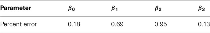
Table A1. Estimated percent errors of the curve-fitting algorithm for 1000 simulated curves.