Meeting the memory challenges of brain-scale network simulation
- 1 Functional Neural Circuits Group, Albert-Ludwig University of Freiburg, Freiburg im Breisgau, Germany
- 2 Bernstein Center Freiburg, Albert-Ludwig University of Freiburg, Freiburg im Breisgau, Germany
- 3 Institute of Neuroscience and Medicine (INM-6), Computational and Systems Neuroscience, Research Center Jülich, Jülich, Germany
- 4 RIKEN Computational Science Research Program, Wako, Japan
- 5 Department of Mathematical Sciences and Technology, Norwegian University of Life Sciences, Ås, Norway
- 6 RIKEN Brain Science Institute, Wako, Japan
- 7 Medical Faculty, RWTH Aachen University, Aachen, Germany
The development of high-performance simulation software is crucial for studying the brain connectome. Using connectome data to generate neurocomputational models requires software capable of coping with models on a variety of scales: from the microscale, investigating plasticity, and dynamics of circuits in local networks, to the macroscale, investigating the interactions between distinct brain regions. Prior to any serious dynamical investigation, the first task of network simulations is to check the consistency of data integrated in the connectome and constrain ranges for yet unknown parameters. Thanks to distributed computing techniques, it is possible today to routinely simulate local cortical networks of around 105 neurons with up to 109 synapses on clusters and multi-processor shared-memory machines. However, brain-scale networks are orders of magnitude larger than such local networks, in terms of numbers of neurons and synapses as well as in terms of computational load. Such networks have been investigated in individual studies, but the underlying simulation technologies have neither been described in sufficient detail to be reproducible nor made publicly available. Here, we discover that as the network model sizes approach the regime of meso- and macroscale simulations, memory consumption on individual compute nodes becomes a critical bottleneck. This is especially relevant on modern supercomputers such as the Blue Gene/P architecture where the available working memory per CPU core is rather limited. We develop a simple linear model to analyze the memory consumption of the constituent components of neuronal simulators as a function of network size and the number of cores used. This approach has multiple benefits. The model enables identification of key contributing components to memory saturation and prediction of the effects of potential improvements to code before any implementation takes place. As a consequence, development cycles can be shorter and less expensive. Applying the model to our freely available Neural Simulation Tool (NEST), we identify the software components dominant at different scales, and develop general strategies for reducing the memory consumption, in particular by using data structures that exploit the sparseness of the local representation of the network. We show that these adaptations enable our simulation software to scale up to the order of 10,000 processors and beyond. As memory consumption issues are likely to be relevant for any software dealing with complex connectome data on such architectures, our approach and our findings should be useful for researchers developing novel neuroinformatics solutions to the challenges posed by the connectome project.
1. Introduction
There has been much development of the performance and functionality of neuronal network simulators in the last decade. These improvements have so far largely been aimed at investigating network models that are at or below the size of a cubic millimeter of cortex (approximately 105 neurons) and within the context of the current dominant laboratory high-performance computing paradigm, i.e., moderately sized clusters up to hundreds of nodes and SMP machines (e.g., Lytton and Hines, 2005; Morrison et al., 2005; Migliore et al., 2006; Plesser et al., 2007; Pecevski et al., 2009). However, there is a growing interest in performing simulations at the scale of multiple brain areas or indeed the entire brain. Firstly, the predictive power of models of the local cortical circuit is severely limited. Such models can account for all the local synapses, but each neuron receives 50% of its synapses from external sources. Thus half of the inputs to the neurons remains unaccounted for, and must be replaced by external currents or random spike input. Secondly, such simulations are a necessary accompaniment to the development of the brain connectome (Sporns et al., 2005), as a structural description of the brain is by definition static. By performing dynamic simulations of the meso- and macroscale networks, we can check the consistency of the anatomical data, integrate it into models, identify crucial missing parameters, and constrain ranges for yet unknown parameters (Potjans and Diesmann, 2011). Thirdly, no part of the brain works in isolation; functional circuits are only closed at the brain-scale. Simulation studies of the interaction of multiple brain areas are necessary to understand how they coordinate their activity to generate brain function. Finally, experimentalists interested in brain function use imaging techniques such as fMRI and MEG and mass recordings such as the LFP to identify the brain’s functional circuits and uncover the dynamics of the interaction between bottom-up and top-down processing. Models of corresponding size are required to create predictions for such measurements.
Brain-scale simulations will necessarily be orders of magnitude larger than the local network models discussed above, and will exceed the capacity of the small-to-medium sized clusters available to researchers within their own research facilities. Fortunately, massively parallel computing architectures installed at dedicated high-performance computing centers are becoming ever more available. In particular, the Blue Gene architectures, incorporating very large numbers of processors with moderate clock speed and relatively small amounts of RAM, provide computational power efficiently, and are consequently increasing in popularity. To exploit these new possibilities for brain-scale simulations, we need simulation software that will scale up to tens or hundreds of thousands of processes. Although very large scale networks have been previously investigated (e.g., Ananthanarayanan and Modha, 2007; Izhikevich and Edelman, 2008; Ananthanarayanan et al., 2009), the underlying simulation technologies have not been described in sufficient detail to be reproducible by other research groups, and so the value of these studies to the neuroscientific community remains somewhat limited.
A major challenge to the scalability of neuronal simulators on such architectures is the limited RAM available to each core. Data structure designs that are reasonable and efficient in the context of clusters of hundreds of processes may be insufficiently parallelized with respect to architectures that are two or three orders of magnitude larger. Insufficient parallelization results in substantial serial memory overhead, thus restricting the maximum network size that is representable on the architecture. We therefore conclude that a systematic approach to understanding memory consumption and designing data structures will be of benefit to any research team attempting to extend the scalability of a neuronal simulator, or indeed any other application, from moderate to very large cluster sizes.
In this manuscript we develop a technique for analyzing the memory consumption of a neuronal simulator with respect to its constituent components on the basis of a linear memory model, extending the approach presented in Plesser et al. (2007). We apply it here to the specific example of the freely available Neural Simulation Tool NEST (Gewaltig and Diesmann, 2007), however the principles are sufficiently general to be applied to other simulators, and with some adaptation to other distributed applications that need to store large numbers of objects. In particular, although we apply the model to a simulator designed for efficient calculation of point neuron models, the technique is equally applicable to simulators optimized for anatomically detailed multi-compartment neuron models. We demonstrate that the model allows the software components that are most critical for the memory consumption to be identified. Moreover, the consequences of alternative modifications to the design can be predicted. As a result of these features, development effort can be concentrated where it will have the greatest effect, and a design approach can be selected from a set of competing ideas in a principled fashion. Finally, we show that this technique enables us to remove major limitations to the scalability of NEST, and thereby increase the maximum network size that can be represented on the JUGENE supercomputer by an order of magnitude.
The conceptual and algorithmic work described here is a module in our long-term collaborative project to provide the technology for neural systems simulations (Gewaltig and Diesmann, 2007). Preliminary results have been already presented in abstract form (Kunkel et al., 2009).
2. Materials and Methods
Typically, memory consumption in a distributed application is dependent not only on the size of the problem but also on the number of processes deployed. Moreover, the relative contributions of the various components of an application to its total memory usage can be expected to vary with the number of processes. To investigate this issue in a systematic way, in the following we develop a model which captures the contributions of the main software components of a neuronal network simulator to the total memory usage (Sec. 2.1). We applied the model to the Neural Simulation Tool NEST. Specifically, the parameterization of the model with theoretically determined parameters (Sec. 2.3) or empirically determined values (Sec. 3.1) is based on version NEST2.0-rc4 using Open MPI 1.4.3 on one core of a 12-core AMD Opteron 6174 running at 2.2 GHz under the operating system Scientific Linux release 6.0.
2.1. Model of the Memory Usage of a Neuronal Network Simulator
Our primary assumption is that the memory consumption on each process is a function of M, the total number of processes:

where 𝓜0(M) is the base memory consumption for an empty network, 𝓜n(M, N) is the memory consumed by N neurons distributed over M processes, and 𝓜c(M, N, K) denotes the additional memory usage that accrues for K incoming synaptic connections for each neuron.
The first term 𝓜0(M) is a serial overhead that consists of the fundamental infrastructure required to run a neuronal network simulator, i.e., the data structures for each process that support the essential tasks sustaining the simulation flow such as event scheduling and communication. It also includes the libraries and data buffers of the message passing interface (MPI) which are necessary for parallelization.
Assuming neurons are distributed evenly across processes and each neuron receives K incoming synapses, NM = N/M neurons and KM = NMK synapses are represented on each process. We previously developed an approximation of the total memory consumption of a neuronal simulator based on the consumption of these objects (Plesser et al., 2007). However, additional data structures may be needed, for example to enable sanity checks during network construction and efficient access to neurons and synapses during simulation. In this manuscript, we will refer to the contribution of these data structures to the memory consumption as neuronal and connection infrastructure, respectively. These data structures are maintained on each process and are a source of serial overhead which increases proportionally with the network size N. Taking into consideration not only neurons and synapses but also the required infrastructures, the memory usage that accrues when creating and connecting neurons is given by:
where mn is the memory consumed by one neuron and mc is the memory consumed by one synapse. The neuronal infrastructure causes  serial overhead per neuron and, additionally,
  per local neuron and
  per non-local neuron. The connection infrastructure causes
  serial overhead per neuron and, additionally,
  per neuron with local targets and
  per neuron without local targets. Our model is based on the assumption of random connectivity. Specifically, each neuron draws K inputs from N possible sources, with repetition allowed. The probability that a neuron i does not select a given neuron j as one of its inputs is (1 − 1/N)K. Therefore, the probability that a given neuron has no local targets on a specific process is given by
  which results in an expected number of
  neurons without local targets on each process. For a specific implementation of a neuronal network simulator, these expressions could be somewhat simplified; for example, the smaller of
  and
and  could be absorbed into
  However, in this manuscript we will be evaluating alternative designs with varying values for these components. We will thus use the full forms of (2) and (3) at all times to ensure consistency.
Our model does not account for any network topology or hierarchy, and it does not consider other types of nodes such as stimulating and recording devices, as the contribution of such devices to the total memory consumption is typically negligible.
2.2. Identification of Simulator Components Contributing to Memory Consumption Terms
Although the aim of this manuscript is to present a general method for analyzing the memory consumption of massively distributed simulation software and planning design alterations, to demonstrate the usefulness of the technique we apply it to the specific example of NEST (Gewaltig and Diesmann, 2007). Figure 1 illustrates the key data structures in NEST that contribute to the parameters of the memory consumption model (2) and (3). Many other simulators are organized along similar lines (e.g., Migliore et al., 2006; Pecevski et al., 2009), however the precise data structures used are not critical for the method. A different design will simply result in different contributions to the memory model parameters.
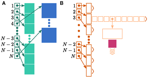
Figure 1. Neuronal and connection infrastructure. The color of elements denotes which memory term they contribute to:  (dark green),
  (mid green), mn (blue),
  (dark orange),
  (light orange), mc (pink). (A) Neuronal infrastructure for M = 4. A
 vector of length N (dark green) is maintained of pointers to either local nodes (blue squares) or Proxy nodes (filled green squares). (B) Connection infrastructure. A vector of length N (dark orange) is maintained of pointers to initially empty vectors (dark orange boxes with single chevrons). If a node makes a synaptic connection to a target on the local machine, the length of the vector is extended to the number of synapse types available in the software (light orange boxes). A GenericConnector object is initialized for the type of the synaptic connection (large light orange box), and a pointer to it laid in the corresponding entry of the vector. The new synaptic connection (pink box) is stored in a deque (four chevrons) within the GenericConnector.
In NEST 2.0-rc4, from hereon referred to as the original implementation, the neuronal infrastructure is organized as a vector of length N on each process of pointers to local nodes and Proxy nodes which represent non-local neurons (see Figure 1A). This structure allows access to neurons on the basis of their unique global identifier, or GID. Access is required for functionality such as setting or querying their variables and connecting neurons. Getting and setting variables does not require the existence of Proxy nodes; assuming the simulation is described by a single serial instruction set, rather than a specific set for each process, all that is required is that each process does nothing when it reads the instruction to manipulate the variables of a non-local neuron. These nodes become important when creating connections, as a Proxy node contains information about the model of the non-local node it is representing. As not all models support all possible types of connection, by querying a Proxy node a process can determine whether a connection specified in its instruction set is valid. In addition to the persistent pointer to each node shown, a second persistent pointer exists that allows a hierarchy of sub-networks to be maintained. It is omitted from all diagrams in this manuscript for clarity. Simulation of the network relies on an additional vector of persistent pointers to local nodes. Thus  comprises the two persistent pointers used for access, mn and
  consist of the size of a local node and the size of a
 Proxy node, respectively, and  is the persistent pointer to local nodes used during simulation.
In NEST, synapses are stored on the same process as their post-synaptic target. When a neuron spikes, its GID is communicated at the next synchronization point to all processes, which activate the corresponding synapses. Certainly for clusters on which the number of machines is less than the average number of post-synaptic targets, this structural organization reduces the bulk of the data to be communicated (Morrison et al., 2005). In the original implementation, the connection infrastructure which mediates the local dispatch of spikes is provided by a vector of length N on each process, as shown in Figure 1B. The contents of the vector are pointers to further structures which contains the synapses sorted by type. The inner structure is a vector which is initially empty; the first time a neuron is connected to a local target, the vector is extended to the length of the total number of distinct built-in and user-defined synapse types. The contents of the vector are pointers to GenericConnector objects which contain deques of synapses of their respective types. This vector of vectors allows the synapses of a particular source neuron, and synapses of a particular type, to be located very quickly. A GenericConnector object for a given synapse type is only instantiated if a neuron actually has synapses of that type. Consequently, the pointer to a vector and the empty inner vector contribute to  mc is the size of a single synapse and
  comprises the pointers to
 GenericConnector objects, the objects themselves and their corresponding empty deques. As there is no representation of non-local synapses,  is zero.
Naturally, other simulation software may not have the constraints described above, or may have additional ones. For example, if all node types support all event types, there is no need to perform validity checking of connections, and the data structures chosen will reflect that. Similarly, if a simulation software has only one type of synapse, no structures are needed to separate different types. Independent of the similarity of the data structures of a specific application to those described above, a careful classification of objects as contributory terms to the different model parameters must be carried out.
2.3. Theoretical Determination of the Model Parameters
We can determine the memory consumptions mn and mc directly by counting the number and type of data they hold. This can either be done by hand, for example by counting 7 variables of type double with 8 B per double, or by using an inbuilt sizeof() function. All neurons derive either directly from the base class Node that takes up 56 B of memory or from the intermediate class ArchivingNode that uses at least 184 B; the greater memory consumption in the latter case is mainly due to a deque that stores a certain amount of the neuron’s spiking history in order to efficiently implement spike-timing dependent plasticity (Morrison et al., 2007).
Many types of neurons and synapses are available within NEST. They vary in the number of state variables and parameters that need to be stored. Hence, mn varies across models. In this manuscript, we will use a leaky integrate-and-fire neuron model with alpha-shaped post-synaptic currents (NEST model name: iaf_neuron), which consumes mn = 424 B. On the 64-bit architecture chosen for our investigations, a pointer consumes 8 B, therefore  (two persistent pointers) and
  (one persistent pointer). The
 Proxy class derives directly from Node without specifying any further data, such that each Proxy consumes 
Similarly, the amount of memory consumed by an individual synapse mc depends on the amount of data stored by the model. We will assume a synapse type that implements spike-timing dependent plasticity that stores variables common to all synapses in a shared data structure (NEST model name: stdp_synapse_hom), such that mc = 48 B. The memory overhead for each potential source neuron is the pointer to a vector (8 B) and the size of an empty vector (24 B), thus  For the sake of simplicity, in this manuscript we will only consider the case that a neuron has exactly one type of outgoing synapse. The additional memory consumption for a neuron with local targets, once the
 vector has been expanded to be able to store the nine built-in synapse types available, therefore consists of 9 × 8 B for pointers to GenericConnector objects and one GenericConnector object of size 104 B, including the empty deque (80 B) that contains the synapses, i.e.,  No additional overhead occurs for neurons that do not have local targets, therefore
3. Results
3.1. Empirical Parameter Estimation
Counting the number of bytes per element or using an inbuilt sizeof() function as in Sec. 2.3 neglects any overhead that a container or the operating system may introduce for the allocation of this memory. Therefore, in this section we measure the actual memory consumption of NEST for a variety of networks to determine the parameters of (2) and (3) empirically; the results are shown in Figure 2.
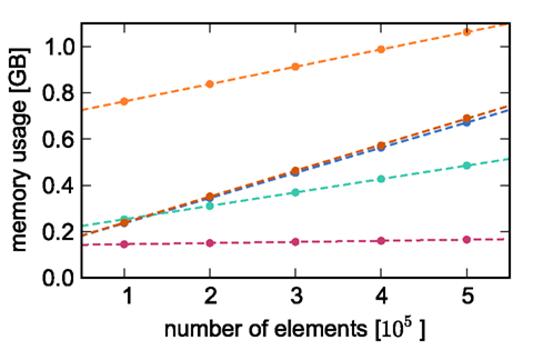
Figure 2. Measured memory usage of simulator components as functions of the number of elements. Memory usage on one process for an unconnected network as a function of the number of nodes (blue circles), an unconnected network distributed over two processes as a function of the number of nodes (green circles), a network with exactly one synaptic connection as a function of the number of nodes (dark orange circles), a single neuron as a function of the number of autapses (pink circles), and a network of 5 × 10⁵ neurons as a function of the number of autapses (light orange circles). The dashed lines indicate linear fits to the respective data sets. All networks created on a single process unless otherwise stated, with neurons of type iaf_neuron and synapses of type stdp_synapse_hom.
To estimate the contribution of MPI to the total memory consumption of NEST at start-up, we compare the measured memory usage when running NEST compiled with MPI support to that used when NEST is compiled without MPI support. On the JUGENE system, we determine that the memory usage of MPI is at most 64 MB and that of NEST 30 MB (for an empty network). For simplicity, we assume a base memory usage of 𝓜0(M) = 94 MB throughout this paper.
To determine the parameters of (2), we create unconnected networks of neurons (type iaf_neuron) on a single process. We increase the number of neurons from 100,000 to 500,000 in steps of 100,000 and measure the memory consumption at each network size. The slope of the linear fit to the data gives the memory consumed by an iaf_neuron object plus the memory overhead per node (local or remote), i.e.,  As the overhead per node consists of two persistent pointers and the overhead per local node of one persistent pointer, in the following we assume
  and mn = 1072 B. Here, we slightly increase the estimate of mn such that it is divisible by eight. To determine the memory usage of
 Proxy representations of non-local nodes, we repeat the measurements for M = 2, such that half of the created nodes are local and half are non-local. Note that memory measurements are still taken on a single process. As mn,  and
and  have already been determined as described above, we can easily extract the amount of memory that is taken up by one
 Proxy node  from the slope of the linear fit, resulting in
  to the nearest multiple of eight.
To parameterize (3), we first repeat the measurements on a single process for increasing network size, with exactly one synaptic connection included at each network size. The existence of a single synapse ensures that the connection infrastructure is initialized but almost entirely empty, similar to Figure 1B. The slope of the linear fit is therefore  resulting in
  to the nearest multiple of eight. We then measure the amount of memory consumed by a single synapse of type
 stdp_synapse_hom by creating one iaf_neuron on a single process with connections to itself. We increase the number of autapses from 100,000 to 500,000 in steps of 100,000 and measure the memory consumption at each network size. The slope of the linear fit to the data reveals mc = 48 B to the nearest multiple of eight. Finally, we determine the additional memory overhead for a neuron with local targets  We create a network of 5 × 10⁵ neurons and successively connect each neuron to itself exactly once. We increase the number of autapses from 100,000 to 500,000 in steps of 100,000 and measure the memory consumption at each network size. The slope of the linear fit to the measurements comprises
  resulting in
  to the nearest multiple of eight. In the original implementation there is no additional overhead for nodes without local targets, therefore
Our results show that the theoretical considerations discussed in Sec. 2.3 do not always accurately predict the true memory consumption. Having made the assumption that the theoretical values for  and
and  are correct, we determine a value for
  which is close to its theoretical value (i.e., 57 B compared to 56 B). However, the empirically measured value for mn is substantially larger than its theoretical value (1074 B compared to 424 B). Similarly, assuming that the theoretical value for
  is correct, we measure values for
  and mc that are near to their theoretical values (35 B compared to 32 B and 50 B compared to 48 B, respectively). The empirically measured value for
  is markedly larger than its theoretical value (700 B compared to 176 B). The fact that the empirically determined values for
  and mc are so close to their theoretical values suggests that it was reasonable to make the assumption that
  and
and  are correctly predicted by their theoretical values.
The empirical values that are well predicted by their theoretical values measure the memory consumption of objects containing only static data structures, whereas the two empirical values that are underestimated by their theoretical values, mn and  measure the memory consumption of objects that also contain dynamic data structures, specifically
 deque containers. The underestimation is due to the fact that dynamic data structures can be allocated more memory when they are initialized than the results of the sizeof() function reveal. In the case of the deque, memory is pre-allocated in anticipation of the first few entries. Increasing the number of autapses for each neuron from one to two does not cause the memory consumption to increase by 48 B per neuron, because the synapses are stored in this pre-allocated memory; a new section of memory is only allocated when the originally allocated memory is full (data not shown). However, this is exactly the extreme case we need to be concerned with for large scale networks/clusters: each neuron having either zero or a very small number of local targets on any given machine. Therefore in the following we will use the empirically determined values, at the risk of a certain inaccuracy for small networks/clusters.
3.2. Analysis of Memory Consumption
On the basis of our model for the memory consumption of a neuronal simulator (Sec. 2.1) with empirically determined parameters (Sec. 3.1), we calculated the usage of memory by NEST for the individual components and in total. Here and in the rest of the manuscript, we assume K = 10,000 synapses per neuron, representing a worst-case connectivity at least for cortical network models. The results for the cases of strong scaling (i.e., fixed network size on an increasing number of processes) and of weak scaling (i.e., network size increases proportionally to the number of processes) are displayed in Figure 3. The strong scaling results demonstrate that although the memory that is consumed by one neuron (mn = 1072 B) is two orders of magnitude greater than the memory that is consumed by one synapse (mc = 24 B), neurons contribute far less to the overall memory consumption. As the number of synapses is four orders of magnitude greater than the number of neurons, the contribution of neurons to the total memory consumption is negligible, whereas the contribution of synapses dominates the total memory consumption for less than around 300–700 processes. At these small-to-moderate cluster sizes, the size of an individual synapse plays a substantial role in determining the maximum neuronal network size that will fit on a given cluster. As the number of processes increases, the relative contribution of the size of synapse objects decreases and the curves for total memory consumption converge.
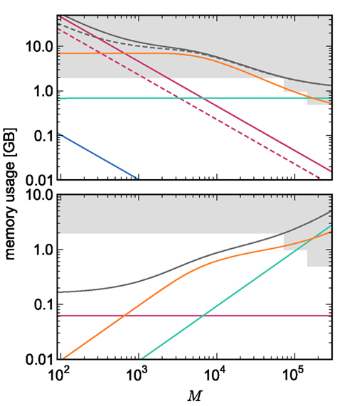
Figure 3. Prediction of component and total memory usage per process as a function of the number of processes. Upper panel: Memory usage for a network containing N = 9.5 × 10⁶ neurons and K = 10,000 synapses per neuron: memory consumed by neurons (blue, mn = 1072 B), neuronal infrastructure (turquoise,  ), synapses (pink), connection infrastructure (orange,
  ), and total memory (gray). Dashed lines show memory consumption using a light-weight static synapse with mc = 24 B, solid lines using a more complex plastic synapse model with mc = 48 B. The gray area indicates a regime that lies beyond the memory capacity of the JUGENE Blue Gene/P machine. Lower panel: Memory usage for a network with NM = 129 neurons on each machine and K = 10,000, such that N = 9.5 × 10⁶ just fits on M = 73,728 processes with 2 GB RAM each. Line colors and shaded area as in upper panel.
For cluster sizes greater than 700, the dominant component of memory consumption is the connection infrastructure; for greater than 3000–7000 processes, the neuronal infrastructure also consumes more memory than the synapses. The neuronal infrastructure is proportional to N for all but very small values of M (2); the connection infrastructure memory consumption is proportional to N up to around M = 10,000 (3). This results in constant terms in the case of strong scaling (Figure 3, upper panel) and linearly increasing terms in the case of weak scaling (Figure 3, lower panel). For M > 10,000 the increase in memory of the connection structure is sub-linear with respect to N, because the number of neurons with no local targets  increases. However, the absolute value of the memory consumption of the connection infrastructure remains very high, and is only overtaken by the consumption of the neuronal infrastructure at around M = 200,000. We can therefore conclude that the serial terms in the memory consumption of neuronal and connection infrastructures represent major limiting factors on the simulation of brain-scale models in NEST.
3.3. Evaluation of Design Strategies
In the previous section we determined that infrastructures, rather than the actual objects of interest in a simulation, are the most memory consuming components for large numbers of processes. In this section we demonstrate that, having identified a problem, the memory modeling approach can be used to predict the effects of design alterations, and thus provide a foundation for deciding on which optimization to focus resources. The commonality between the issues of neuronal infrastructure and connection infrastructure is that as network and machine sizes increase, the infrastructures become increasingly sparse. For a network containing N = 9.5 × 10⁶ neurons on M = 73,728 processes with 2 GB RAM each, there are only 129 neurons on each machine (see Figure 3) and thus almost 9.5 × 10⁶ entries in the neuronal infrastructure to account for non-local neurons. Similarly, under the assumption of random connectivity, around 87% of neurons will not have any local targets on a given machine. Thus, taking this sparseness into consideration will help to avoid serial overheads that grow with the network size. Note that for smaller clusters and network sizes, sparseness is not a major consideration. For less than around 700 processes, the serial overheads are dominated by the memory consumption of synapses. In this regime, it is reasonable to use data structures that do not exploit sparseness.
There are two requirements on data structures to replace the neuronal and connection infrastructure. The first requirement is that memory overheads for non-present items are extremely low, so that sparseness is effectively exploited. The second requirement is that the data structures enable efficient search routines. This requirement is based on the assumptions that a distributed simulation described by a single serial instruction set, or script, and that a pre-synaptic spike is delivered to all processes and then dispatched to the local targets. If the former assumption is false, then it is not necessary to search the neuronal infrastructure for neurons that may be located on other machines. If the latter is false, it is not necessary to search the connection infrastructure for local targets of a neuron that may not have any on that specific process. If the assumptions are true, the requirement is that a search routine exists for the candidate data structure that terminates rapidly, both when a searched-for item is present and when it is not present. The original implementation of the neuronal infrastructure, consisting of a vector of pointers to local neurons and proxies of non-local neurons, fulfills the second requirement but not the first. A well-loaded hash map fulfills the first requirement but not the second, as the worst-case look-up time (which can be expected to occur frequently for high degrees of sparseness) is 𝒪(n) for typical implementations, where n is the number of items stored. The worst-case look-up time has been improved to 𝒪(log n) and even 𝒪(1) but at the cost of higher memory consumption (Dietzfelbinger et al., 1994). Two candidates which fulfill both requirements are sparse tables (Silverstein, 2005) and cuckoo hash maps (Pagh and Rodler, 2004).
Sparse tables store entries in groups of equally sized successive index ranges; by default sgr = 48 entries per group with an overhead of mgr = 10 B per group; each group contains a contiguous block of entries and a bitmap of size sgr, which indicates whether there is an entry for the given index or not; to store entries with maximum index n the total overhead of the sparse table (i.e., not including the memory consumption of the stored items) is n(mtest + mgr/sgr) where mtest = 1 bit.
Cuckoo hashing is an interesting alternative to standard hashing as it provides a look-up time that is constant in the worst-case (Pagh and Rodler, 2004). In its original formulation it consists of two hash functions and two hash tables. To store an item x, the first hash function is used to generate a location. If the location is already occupied by an item y, the new item x replaces the stored item y, and the second hash function is used to generate a location for item y in the second hash table. Should this location also be occupied by an item z, the items are swapped, and then the first hash function is used to generate a location for the displaced item z in the first hash table. The process continues, alternating hash functions and tables, until an empty location is found or a predefined maximum number of iterations is reached. In the latter case, a rehash is performed. This concept was later extended to d-ary cuckoo hashing, i.e., d hash functions that code for alternative positions in one hash table, where the capacity threshold ch depends on the number of hash functions: ch = 0.49, 0.91, 0.97, 0.99 for d = 2, 3, 4, 5 (Fotakis et al., 2003). In common with other imperfect hashing schemes, i.e., where there is no guarantee that the hash function will generate a unique location for each key, the keys need to be stored with the items to allow identification at look-up time. This results in an overhead of mkey per entry. To store n entries the hash size should be at least n/ch, which entails a total memory usage (i.e., including the memory consumption of the stored items) of n(mkey + mval)/ch, where mval is the memory consumption of payload per entry. In the rest of the manuscript, we will consider tertiary cuckoo hashing schemes (ch = 0.91).
3.3.1. Neuron infrastructure
Let us first consider an alternative approach to implementing the neuronal infrastructure. The infrastructure has two critical functions, related to access and connection, respectively. Firstly, it has to enable a rapid determination of whether a given global index (GID) refers to a local or remote node, and return a pointer to the node if it is local. In the original implementation of the neuronal infrastructure, this functionality is ensured by a vector of pointers to local neurons and proxies for the non-local neurons (Figure 4A). The locality of a node with a given GID can be determined very quickly, as the GID of a node determines which index of the vector to examine. If following the pointer results in a non-proxy node, then by definition the node with that GID is local. Conversely, if following the pointer results in a Proxy node, then the node is non-local. Similarly, returning a valid pointer once a node has been determined to be local is trivial.
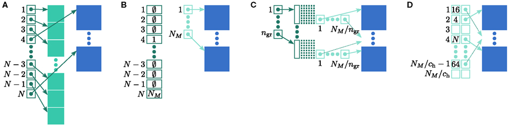
Figure 4. Alternative designs for the neuronal infrastructure. In all panels M = 4, and the color of elements denotes which memory term they contribute to:  (dark green),
  (mid green),
  (light green), mn (blue). (A) Original implementation. A
 vector of length N (dark green) is maintained of pointers to either local nodes (blue squares) or Proxy nodes (filled green squares). (B) Look-up tables implementation. A vector of length N (dark green) is maintained that contains the local indices in a vector of length NM (light green) for local nodes and a special value (here ∅) for remote nodes. The shorter vector contains pointers to the local nodes. (C) Sparse table implementation. A vector of length ngr (dark green) is maintained of pointers to sparse groups, that is ngr = N/sgr denotes the number of sparse groups. A sparse group has an overhead of mgr (vertical dark green boxes) and sgr bits (tiny dark green squares) that are set to 1 if an item is present at the given index and 0 if it is absent. The NM/ngr local items in each group (light green squares) are pointers to local nodes. (D) Cuckoo hashing implementation. A hash table of size NM/ch (light green squares) is maintained that contains pointers to local neurons as payload and also the keys of the items (i.e., the global indices of the stored nodes).
Secondly, as not all neuron models support all possible connection types, the neuronal infrastructure must allow the model of a node with a given GID to be determined, independent of whether it is local or remote. In NEST a model is a separate object from the nodes it creates. Local nodes and Proxy nodes explicitly store a model index (MID), which can be used to access a local model object. Therefore, Proxy nodes can uniquely identify the model of their remote counterparts. With access to this information, a process can check whether a connection described in the instruction set is valid.
One strategy to exploit the sparseness in the neuronal infrastructure is to use look-up tables. A vector of size NM that stores pointers to local neurons is maintained, see Figure 4B. This is supplemented by a look-up table of size N that maps a node’s GID to its local index in the node vector if it is local, and to a special value if it is remote. This enables a swifter determination of node locality, as fewer indirections are involved. Returning a valid pointer to a local neuron is also trivial in this design. To access the type information of a non-local neuron, an additional look-up table can be used that maps ranges of GIDs to their MID. Usually ranges for a given MID can be expected to be quite large, as it is substantially more convenient to create blocks of neurons of the same model than to create them individually whilst varying models. Thus the MID for a given GID can be obtained by performing a divide-and-conquer search of a table that is expected to be several orders of magnitude smaller than N. As the memory consumed by the model look-up table is negligible, the memory usage of the neuron infrastructure when using look-up tables is given by (2) where  now accounts for the size of the data type that stores the local index of nodes in the node look-up table, and
  accounts for the two persistent pointers to local neurons used for access and the one persistent pointer used during simulation. As there are no proxies,
An alternative strategy is to replace the vector of pointers to nodes and proxies with a sparse table that stores pointers to local neurons, and represents with one extra bit whether an item is present (local) or absent (remote). This is depicted in Figure 4C. As with the previous strategy, this enables a swift determination of locality and return of valid pointers to local neurons. Similarly, this data structure must be supplemented with a model look-up table to provide access to the models of remote nodes. The memory usage for this design is as in (2) with  where mtest = 1 bit, and sgr = 48 and mgr = 10 B are the sparse table group size and memory overhead per group as discussed above,
  and
and 
A third strategy is to use cuckoo hashing to store the pointers for local nodes, as shown in Figure 4D, which reduces the overhead per neuron to  The memory usage for this design is therefore given by (2) with
  . Here, mkey = 4 B is the data type of the key, i.e., the GID of a node (for ranges up to 109), mval = 8 B is the payload, i.e., the size of a persistent pointer to a node, and ch = 0.91 is the capacity threshold of the hash map as discussed above. The final term of 16 B accounts for the two additional persistent pointers to each local neuron. Also in this design, the total removal of proxies results in
All three strategies remove the need for the concept of a Proxy node which stands in for its remote counterpart to fulfill various roles in the simulator functionality. The ideal memory usage for neurons would be (2) with  i.e., no neuronal infrastructure to account for non-local neurons and no persistent pointers required for local neurons. By calculating the memory usage as a function of the number of processes assuming the three strategies above, we can see to what extent these strategies deviate from the ideal case. This is displayed in Figure 5. All three strategies result in reduced memory consumption with respect to the original design described in Sec. 2.3, for all values of M. For M < 1000 both the look-up table and the sparse table design are close to ideal. For M > 1000, the sparse table design results in a greater reduction of memory consumption with respect to the original implementation, and is in fact very close to optimal. The cuckoo hashing design gives very similar results to the sparse tables design for M < 100,000, but marginally improved results for greater numbers of processes (data not shown). As sparse tables and cuckoo hashing result in a more substantial improvement in memory consumption than look-up tables for M > 1000, we can discard look-up tables as a design candidate. We can further conclude that the improvements to memory consumption obtained by cuckoo hashing compared to sparse tables do not compensate for their greater complexity. Thus, we conclude that a sparse table combined with a light-weight model look-up table is the best of the three strategies to reduce the memory footprint of the neuronal infrastructure.
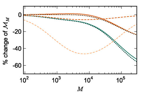
Figure 5. Prediction of change in memory usage per process for infrastructure components for different design choices with respect to the memory usage of the original design. Percentage change of the total memory usage for a network of NM = 1000 neurons on each process predicted as a function of the number of processes when implementing neuronal infrastructure as a look-up table (dark green) or a sparse table (light green) and when implementing connection infrastructure as a hash map with capacity threshold ch = 0.91 (solid dark orange) or a sparse table (solid light orange). The dotted black curves show the ideal cases that there is no memory overhead for neuronal infrastructure,  and no memory overhead for connection infrastructure,
  Assuming no optimizations to exploit sparseness are carried out, the dashed light orange curve shows predicted change to memory usage for synapses stored in
 vectors instead of deques, and the dashed dark orange curve indicates the predicted change for synapses stored in deques, for a reduced size of the vector containing pointers to GenericConnector objects.
3.3.2. Connection infrastructure
The functionality that any implementation of the connection infrastructure must deliver is as follows. Firstly, it must be able to mediate spikes that are communicated to the process. Assuming that each arriving spike event knows the GID of the neuron that produced it (Morrison et al., 2005), the connection infrastructure must be able to determine rapidly whether the node corresponding to that GID has local targets. If so, it must provide access to the synapses that communicate the spiking information from the node to its targets. If communication between processes is implemented such that spikes are guaranteed to be sent only to processes on which they have targets, rather than to all processes, this requirement can be relaxed to swift access to the local synapses of a given node GID, without the initial determination of their existence.
As synapses can be of heterogeneous types, in order to allow the user to query the state of the network it must also be possible to locate all synapses of a given type for a given pre-synaptic node GID. The original implementation of the connection infrastructure, as shown in Figure 6A, consists of a vector of length N of pointers to vectors of pointers to GenericConnectors, one per type of synapse that the node makes to local targets. The GenericConnectors contain deques of synapses of their respective types. Therefore the existence of local targets for a node with a given GID can easily be determined by testing whether the pointer in the vector of length N at index GID points to a non-empty vector. Allowing access to the relevant synapses is then trivial. As the synapses are sorted into vectors according to their types, searching for particular synapses of a particular type for a given node is straightforward.
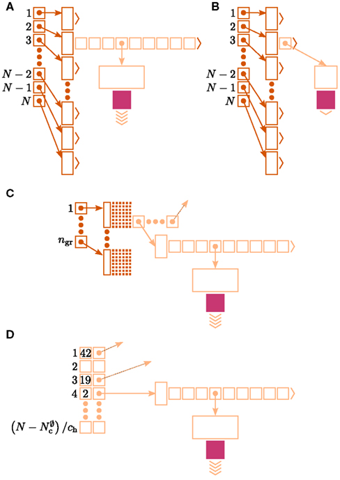
Figure 6. Alternative designs for the connection infrastructure. The color of elements denotes which memory term they contribute to:  (dark orange),
  (light orange), mc (pink). (A) Original implementation. A
 vector of length N (dark orange) is maintained of pointers to initially empty vectors (dark orange boxes with single chevrons). If a node makes a synaptic connection to a target on the local machine, the length of the vector is extended to the number of synapse types available in the software (light orange boxes). A GenericConnector object is initialized for the type of the synaptic connection (large light orange box), and a pointer to it laid at the corresponding index of the vector. The new synaptic connection (pink box) is stored in a deque (four chevrons) within the GenericConnector. (B) Light-weight internal structure implementation. As in (A), but the vector of synapse types is only as long as the number of synapse types a node actually has on the local machine, and synapses are stored in a vector (single chevron) rather than a deque, which decreases the size of the GenericConnector. (C) Sparse table implementation. A vector of length ngr (dark orange) is maintained of pointers to sparse groups, that is ngr = N/sgr denotes the number of sparse groups. A sparse group has an overhead of mgr (vertical dark orange boxes) and sgr bits (tiny dark orange squares) that are set to 1 if an item is present at the given index and 0 if it is absent. The local items in each group (light orange squares) are pointers to vectors of GenericConnector objects and their respective deques of synapses (light orange/pink), as in (A). (D) Cuckoo hashing implementation. A hash table of size  (light orange squares) is maintained that contains the keys of the items (i.e., the global indices of the pre-synaptic nodes) and as payload, pointers to
 vectors of GenericConnector objects and their respective deques of synapses (light orange/pink), as in (A).
Figure 5 shows that improvements in memory consumption can be obtained by reducing the additional memory overhead for nodes with local targets,  Storing synapses in
 vectors instead of deques reduces memory consumption substantially up to a maximum of 46% at around M = 7000, after which the amount of improvement reduces for larger M. For M < 50,000, this adaptation results in greater improvements to the memory consumption than exploitation of sparseness in the neuronal or connection infrastructure. To make this prediction, we estimated  for the case that a
 GenericConnector object contains its synapses in a vector. An empty vector consumes 24 B in comparison to 80 B for an empty deque, therefore the theoretical value for  reduces from 176 B to 120 B. However, as discussed in Sec. 3.1, the theoretical values can substantially underestimate the actual values; we measured
  which implies that the
 deque is approximately seven times larger than its theoretical value. This is likely to be less problematic for vectors than for deques, as the memory allocation of vectors is more straightforward. We therefore make a pessimistic estimate of  assuming that a
 vector also consumes seven times more memory. However, any reasonable estimate would produce qualitatively similar results. We therefore conclude that implementing synapse containers as vectors rather than deques is a useful step to improve the memory consumption. A lesser degree of improvement can be achieved by reducing the size of the vector of pointers to GenericConnector objects. Instead of one entry for each available synapse type, the length of the vector can be reduced to the number of synapse types the source neuron actually has on the local machine. This necessitates increasing the size of the GenericConnector object to include a synapse type index. This adaptation results in a maximum of 6% improvement for 7000 processes. Figure 6B illustrates the strategies for reducing  which are described above.
Disregarding potential improvements to the  component, we can also consider how to exploit the sparseness of the distribution of synapses over the machine network. One possibility to account for the increasing number of neurons without local targets is to replace the
 vector of length N with a sparse table, as shown in Figure 6C. This allows very rapid determination of whether a node has local targets; if local targets exist, access to the corresponding synaptic connections is also swift. For nodes with local targets, the internal structure of a vector of pointers to GenericConnectors is maintained, to allow per-type storage of synapses. The memory usage for this design is as in (3) with  and
and  Note that
  has absorbed 32 B from
  in the original implementation. This accounts for an empty
 vector (and pointer to it) which is now only initialized for nodes which have local targets, rather than all nodes.
As with the neuronal infrastructure, an alternative design strategy is cuckoo hashing. The hash table contains  items, where
  is the number of nodes with local targets, therefore a table of size
  is required. Each item consists of a pointer to a
 vector of pointers to GenericConnector objects, i.e., the same internal structure as in the original implementation. As for the neuronal infrastructure in Sec. 3.3.1, the keys of the items, in this case the GIDs of the pre-synaptic neurons, must be stored with the items. This is illustrated in Figure 6D. In this case, total memory consumed by synapses and connection infrastructure is given by (2) with  where mkey = 4 B, mval = 8 B, and ch = 0.91.
The ideal memory usage would be for the case that there was no infrastructure overhead for neurons without local targets, i.e., as in (3) with  and
and  Figure 5 shows the predicted deviations of the sparse tables and cuckoo hashing strategies from the ideal case as a function of the number of processes M. For M < 4000 neither strategy improves memory consumption with respect to the original implementation; sparse tables require approximately the same amount of memory, and cuckoo hashing requires slightly more. This is because, unlike the situation with the neuronal infrastructure, there is no sparseness to be exploited on small numbers of processes. Assuming each node selects K pre-synaptic source nodes from a total of N nodes distributed evenly on M machines, the probability that a given node has no targets on a given machine is
  With K = 10,000 and N ranging between 105 and 3 × 10⁸ as in Figure 5, 5% of the connection infrastructure is empty for M = 3338, 50% of the connection infrastructure is empty for M = 14,427, and 95% of the connection infrastructure is empty for M = 194,957. For M < 350,000 the sparse table design results in a greater improvement to the overall memory consumption with respect to the original implementation than the cuckoo hashing design, and is in fact close to ideal. For larger values of M, the cuckoo hashing design results in marginally better memory consumption. Due to the better performance of the sparse table implementation for numbers of processes in the relevant range and the greater complexity of cuckoo hashing, we conclude that a sparse table is the better of the two designs for exploiting sparseness in the connection infrastructure for M > 3000.
3.4. Analysis of Limits on Network Size
In this section, we investigate to what extent the improvements to the memory consumption identified in Sec. 3.3.1 and Sec. 3.3.2 increase the maximum problem size that can be represented on a given machine. Table 1 summarizes the parameters of the memory consumption model for the original implementation (see Sec. 2.2) and the parameters after adaptation of the data structures. The adapted values are for the case that sparse tables are used to implement neuronal and connection infrastructure. Moreover, synapses are contained in vectors rather than deques, and the length of the vector of pointers to GenericConnector objects has been reduced as suggested in Sec. 3.3.2. The empirical memory measurements for the adapted data structures are carried out as described in Sec. 3.1. The memory consumption for a neuron and synapse remain constant, mn = 1072 B and mc = 48 B. Once again, we see that the empirical value for  (136 B) exceeds the theoretical value (96 B) due to the presence of a dynamic data structure, but the discrepancy for a
 vector is not as large as that for a deque in the original implementation. The empirical value for  is less than the theoretical value whereas the empirical value for
  is greater, although they are measuring the overhead of the same type of data structure. This is likely to be due to the limits of measurement accuracy, as the expected value is so small.
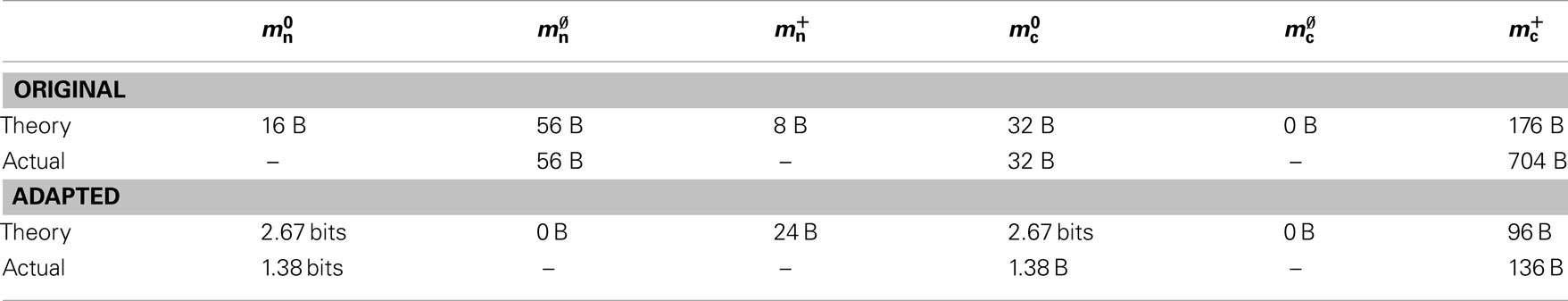
Table 1. Parameters of the memory model. The theoretically and empirically determined parameters of (2) and (3) for the original implementation and the adapted implementation. All empirical values in bytes given to the nearest multiple of eight; empty entries indicate that the corresponding theoretical value was assumed to be accurate to enable determination of other parameters in that row.
Figure 7A shows the predicted memory required for the infrastructure components and the total memory consumption as a function of the number of processes M for two networks. With 1056 neurons on each process, the maximum network size is 7.8 × 10⁷, which just fits on 73,728 processes with 2 GB RAM each, i.e., using one core per machine node of JUGENE. Using the original implementation, the largest network that could be represented with 1056 neurons per process would be 1.7 × 10⁶ neurons on 1642 processes with 2 GB RAM each. With a load of 129 neurons on each machine, a maximum network size of N = 9.5 × 10⁶ is predicted (see Figure 3). Thus, the maximum network size that can be represented on the available machine has increased by an order of magnitude. In addition, the improved infrastructures allow a much more effective use of the entire machine. A network of 5.9 × 10⁷ neurons can be distributed over all 294,912 cores of JUGENE (0.5 GB RAM each) with a load of 201 neurons per core (Figure 7). For the original implementation, the maximum network size that could be represented on the entire machine is 3.1 × 10⁶ neurons with a load of 10 neurons per core, thus the adaptations have increased the size of the network representable on the entire machine by a factor of nearly twenty.
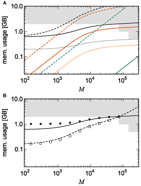
Figure 7. Prediction and measurement of total memory usage per process. (A) Predicted memory usage as a function of the number of processes for a network of NM = 1056 neurons on each machine such that N = 7.8 × 10⁷ just fits on M = 73,728 processes with 2 GB RAM each. Solid curves indicate the memory usage for the adapted implementation, and dashed curves the original implementation. Usage shown for neuronal infrastructure (dark green), connection infrastructure (dark orange), and total memory (black). Dashed curves indicate memory consumption predicted using the original data structures to implement infrastructure. The light orange curve indicates the memory consumption of the connection infrastructure and the light gray curve indicates the total memory consumption for a network with NM = 201 neurons such that N = 5.9 × 10⁷ just fits on M = 294,912 processes with 0.5 GB RAM each. (B) Measured memory usage as a function of the number of processes. Original implementation: memory consumption for a network of NM = 129 neurons on each machine such that N = 9.5 × 10⁶ just fits on 73,728 processes (open circles). Adapted implementation: memory consumption for a network of NM = 1056 neurons on each machine such that N = 7.8 × 10⁷ just fits on 73,728 processes each (filled circles). The theoretical predictions of memory consumption for these networks are given by the dashed and solid curves, respectively.
The memory consumption model accurately predicts the actual memory usage of NEST. Figure 7B shows the memory required per process for a simulation in which each neuron receives 10,000 randomly chosen inputs. As predicted, the largest network that could be represented on JUGENE using the original implementation contains 9.5 × 10⁶ neurons distributed over 73,728 processes with 2 GB RAM each. The measured memory consumption for the corresponding weak scaling experiment with 129 neurons per process is well fitted by the theoretical prediction. As for the previous measurements, these results are obtained on a single core by falsely instructing the application that it is one of M processes. Thus, it only creates the desired N/M local neurons, but all infrastructures are initialized on the assumption that there are an additional N − N/M neurons on remote processes. When using the adapted implementation, the maximum network size on 73,728 processes increases to 7.8 × 10⁷ neurons. The memory consumption for the corresponding weak scaling experiment with 1056 neurons per process is well fitted by the theoretical prediction for M > 2000. For smaller numbers of processes, the model underestimates the true memory consumption. This is due to the vectors containing the synapses doubling their size when they are filled past capacity, thus allocating more memory than is strictly needed. As the number of local synapses per source neuron decreases, the vectors are more optimally filled, leading to a convergence of the measured memory consumption to the theoretical prediction. A better fit can be obtained by accounting for the sub-optimal filling of vectors in the model, but as we are more concerned with correct prediction of the model for large numbers of processes, we omit this extension of the model for the sake of simplicity. Note that this effect does not occur for the original implementation, as the synapses are stored in deques, which allocate memory in constant-sized blocks.
The shallow slope of the memory consumption curve for the adapted implementation means that doubling the number of available processes will approximately double the size of the network that can be represented to 1.5 × 10⁸. In sharp contrast, the steep slope of the memory consumption curve for the original implementation means that doubling the machine size would only increase the size of the maximum network to 1.2 × 10⁷, a factor of 1.3.
The adaptations to the data structures alter not only the absolute memory usage of the various components of NEST, but also the relative usage. Figure 8 shows the proportion of the total memory consumed by each of the components in the original and the adapted implementation. The cross-over point at which the neuronal infrastructure requires more memory than the synapses is eliminated in the adapted implementation; the memory consumption for the neuronal infrastructure is essentially negligible for a large range of processes, having been reduced to under 3 bits per node. The point at which the memory usage of the connection infrastructure is greater than that of the synapses is shifted from M = 700 for the original implementation to M = 4000 for the adapted implementation. However, even this shifted value is comparatively low with respect to the number of processes available on a large Blue Gene machine. At M = 200,000, the connection infrastructure accounts for nearly 70% of the total memory usage, synapses for just over 20%, and neurons approximately 5%. It is therefore clear that any further increases to the maximum network size that can be simulated on a machine with in the order of 100,000 processes can only be achieved by further reducing the overhead for the connection infrastructure. Given that the connection infrastructure also exploits the sparseness of the distribution of synapses over the processes, the question arises of why it is still the dominant memory component for large M. The answer is that although the first term of (3) has also been reduced to less than 3 bits per node and so is negligible, the third term  is not. This term expresses the memory consumption of the data structure containing the synapses with local targets, which is comparatively large,
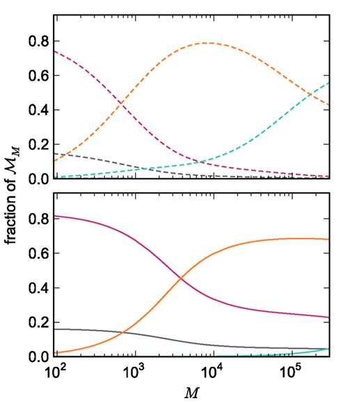
Figure 8. Relative memory consumption per process as a function of the number of processes. Fraction of total memory consumption predicted for the following components: NEST and MPI (gray), synapses (pink), connection infrastructure (orange), neuron infrastructure (green) for the case that the number of neurons per process is set to NM = 1000. Upper panel: original implementation. Lower panel: adapted implementation.
The potential benefits of reducing  are illustrated in Figure 9, which shows the largest network size that could be represented as a function of the number of processes. The original implementation shows a saturating behavior, whilst the adapted implementation shows an approximately linear relationship. The ideal case is that there is no memory overhead for neuronal or connection infrastructure. By reducing the overhead for neurons with local targets from
  to 16 B, a close to optimal performance could be achieved. Therefore we can conclude that the next priority for reducing memory consumption should be optimizing this aspect of the connection infrastructure, rather than reducing the sizes of the neuron and synapse objects themselves, or attempting to further exploit sparseness in the data structures.
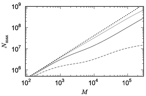
Figure 9. Prediction of maximum network size as a function of the number of processes. Original implementation (dashed curve), adapted implementation with  (solid dark gray curve), adapted implementation assuming
  (solid light gray curve). The dotted curve indicates the predicted maximum network size for the ideal case, i.e., no overhead for neuronal or connection infrastructure
  Curves are based on the assumptions of 2 GB RAM per process and 10,000 incoming connections per neuron.
4. Discussion
Saturation of speed-up at distressingly low numbers of processes is a very common experience when parallelizing an initially serial application, occurring when the contribution of the serial component of an algorithm to the total computation time outweighs that of the parallel component. Here, we consider the analogous problem of saturation of the available memory, which occurs when serial components of data structures consume all the memory available for each process, such that increasing the number of processes available does not increase the size of the problem that can be represented. The shift from saturation in computation time to saturation in problem size may be a characteristic of technological progression: an algorithm that performs perfectly well in a serial program may be poorly designed with respect to later parallelization, i.e., has large serial computational overhead. Re-designing algorithms with the previously un-dreamed-of parallelization in mind results in better parallel algorithms and extends the realm of scalability to much higher numbers of processes. When trying to extend the realm of scalability to ever larger problems and cluster sizes, a data structure design that performs perfectly well on the moderate scale may turn out to be poorly designed with respect to massive parallelization, i.e., it contributes a substantial serial term as well as a parallel term to the total memory usage. The serial overhead is not noticeable or problematic on moderate scales, but becomes dominant on large scales, resulting in a constant term in strong scaling investigations and a linear term in weak scaling investigations.
To analyze this problem in a systematic fashion, we developed a model for the memory consumption of a neuronal simulator which allows us to separate serial and parallel contributions. In this manuscript we apply the model to understanding and improving the memory consumption of NEST (Gewaltig and Diesmann, 2007). This entails taking the constraints of NEST’s fundamental design into consideration, for example that it must be possible to determine the model of every node, regardless of locality, and that spikes are distributed to all processes and then dispatched by the local synapses. However, the expressions are general enough to be used for any neuronal simulator, in particular those developed to simulate networks of complex compartmental neuron models. For a given simulator, the data structures of the simulator must be analyzed to determine which objects contribute to which parameters of the memory model. If a simulator has different underlying constraints from NEST, this will reduce or expand the range of possible data structures that can be considered as alternative designs. The role of the model is to evaluate the consequences of potential design choices in terms of memory consumption, not to identify the range of possible solutions. Moreover, the principles are applicable to any distributed application that needs to maintain a large number of objects, although in such cases the terms of the memory model would have to be adapted.
By empirically determining the parameters of the model, we found that the theoretical values for the memory consumption of some data structures underestimate their actual memory consumption. In particular, dynamic data structures typically use more memory than would be predicted by the sum of the size of the empty structure and the size of their contents, due to the dynamic allocation of memory. The additional memory overhead of dynamic data structures depends on their type and size. A deque from the C++ standard template library typically allocates a section of memory that is substantially bigger than that needed to store a single element. As further elements are stored, the total memory consumed does not increase until all that memory is filled. It then allocates another section of the same size. Therefore, deques are not a good choice for storing small numbers of elements if conserving memory is important. The typical strategy for a vector from the standard template library is to initially allocate little or no memory for storage. When the capacity of the vector is exceeded, the memory allocation is doubled. As a result, vectors are memory efficient for storing small numbers of items, but for large numbers the difference between the allocated memory and the desired memory can be quite substantial. This discrepancy can be eliminated if the number of items to be stored is known in advance. At present, network models tend to be expressed in terms of connection probabilities or distributions of the number of incoming or outgoing synapses. Consequently, whereas it is generally possible to predict the number of neurons in a network model, the same is not true for the number of synaptic connections a neuron makes to targets on a specific machine.
Using the empirically parameterized model, we found that the ranking of components of the simulator with respect to their memory consumption varied with the numbers of processes. For tens to hundreds of processes, synaptic connections account for most of the memory consumption in a fixed size problem. At around 700 processes, the connection infrastructure that allows the synapses to be stored and accessed becomes the most dominant component, followed by the neuronal infrastructure at around 7000 processes. This analysis revealed that serial terms of the infrastructure components cause a saturation in the scalability of the simulator with respect to memory consumption.
As well as analyzing the memory consumption for the implemented data structures, we showed that the technique can also be applied to predicting memory consumption for alternative designs. These two features enable us to determine, in a principled fashion, which components are the highest priority to be improved, and which of multiple competing design strategies will be most effective. By comparing the memory consumption of potential designs to ideal cases, i.e., where there is no overhead for infrastructure, it is also possible to determine if there is anything more to be gained by improving a given data structure.
Whereas this approach would be useful for any range of processes, it is particularly helpful for large values of M. Without a principled approach to analyzing memory consumption as described here, developers are reduced to assumptions and intuition. These can both be misleading, especially for extremely large numbers of objects with a high degree of sparseness, resulting in long development cycles and wasting precious time allocations on supercomputers.
In the case of NEST, we discovered that exploiting sparseness in the neuronal and connection infrastructures was the most promising way to reduce memory usage, rather than, for example, reducing the size of neurons or synapses. It turned out that a design based on sparse tables results in greater improvements to the memory consumption than one based on look-up tables. A design based on cuckoo hashing consumes a similar amount of memory to a sparse table design, but is more complex. Therefore, we selected sparse tables as the most memory efficient strategy to exploit sparseness. Reducing the memory overhead for neurons with local synapses  was also useful, indeed for architectures with a number of processes less than 50,000, this is the single most effective way to reduce memory consumption. Taken together, these adaptations increased the maximum network size that can be represented on the JUGENE supercomputer by an order of magnitude. This is assuming a high number of synapses per neuron – our calculations are based on K = 10,000 throughout. Clearly, a lower value would allow larger networks to be represented. Similarly, the assumption of random connectivity represents a worst-case, as it results in neurons typically having zero or one synapses on a given process. Topological considerations that result in fewer and longer lists of outgoing synapses for a given source neuron will also decrease the memory consumption, and so allow larger problems to be represented.
Meso- and macroscale simulations will for the next 10 years be bound to very large scale hardware, where scientists depend on using the architectures they have access to at computer centers. To be a useful tool, freely available simulators such as NEST need to work efficiently across a range of such architectures, as opposed to being optimized for a given architecture (e.g., Ananthanarayanan and Modha, 2007). This requires them to have a design that allows infrastructure optimizations without affecting user- and model-developer interfaces, models of the software, e.g., its memory consumption as developed here, to provide an understanding of bottlenecks and help in prioritizing optimizations, and a modular design that separates concerns as much as possible. The benefit of such a modular design is adequately demonstrated by the fact that we could perform all the described adaptations without requiring any changes at the user or model-developer level. Ultimately, the increasing range of hardware sizes may demand greater flexibility in the design of data structures, such that the size of the hardware determines which data structures are used at either compile or run-time. In the absence of the constraint of flexibility across architectures, a further use of the memory model is to help prioritize development resources with respect to a particular intended problem or machine. For example, for maximum cluster sizes below 10,000, exploiting sparseness could be considered a priority for the neuronal infrastructure but not for the connection infrastructure (see Figure 5).
Irrespective of the range of M for which the application should exhibit good performance, in general, trade-offs must be negotiated between memory consumption and computation time. Current trends indicate that hardware will move to increasingly multicore designs with massive processing power and limited and slow memory. Our adaptations here reflect this trend, as we replace algorithmically simple but memory-demanding representations with compact, but algorithmically more complex representations. For example, storing data in a hash table rather than a vector requires applying the hash function to the item key to determine its location in the table, which is computationally more expensive. Similarly, one can imagine a design where synapses are not addressable by the index of the pre-synaptic neuron, as in all potential designs considered here, but in a contiguous block of all synapses of the same type. This would reduce the memory overhead for neurons with local targets substantially, but would necessitate additional indirections or a searching strategy to locate the outgoing synapses for a given neuron and thus may increase the run-time. On the other hand, reducing the memory footprint can increase cache efficiency and thus decrease the run-time, despite additional indirections. The model we have proposed here does not account for computation time, and thus cannot predict these effects.
In Morrison et al. (2005) we presented the data structures and algorithms that allow networks in the order of 105 neurons with 109 synapses to be routinely simulated on small clusters. As a result, local cortical networks with realistic connectivity and sparseness could be studied for the first time. Here, we develop adaptations to those data structures that allow networks of the order of 107 neurons and 1011 synapses to be simulated on a popular modern supercomputer architecture, the Blue Gene, whose characteristics are a very large number of processors and a modest amount of RAM per core. These advances allow networks with macroscopic connectivity to be studied, in which some functional circuits are closed and the majority of synapses are accounted for. Networks of 108 neurons and 1012 synapses are also realizable, by either increasing the number of cores available, or reducing the overhead for neurons with local targets  see Figure 9.
However, we are then still about three orders of magnitude away from the human brain. What are the next challenges, assuming the trends of increasing number of cores but low RAM per core continue? If 1 GB per core is a reasonable prediction of the amount of memory available for each core, the next decisive barrier is at 109. Although we have reduced the serial overhead in the neuronal and connection infrastructure to a matter of a few bits by using sparse tables, when the number of neurons approaches the number of bytes available in a core’s RAM, these serial terms will dominate the total memory consumption and cause the maximum network size to saturate. Therefore, data structures must be implemented that eradicate any serial overhead, at the cost of a greater number of computational operations required to test whether neurons are local or have local targets, and also to access the objects that are stored locally. By this size the degree of sparseness is so great that all-to-all communication would be extremely inefficient. A more sophisticated approach to route the exchange of spikes between neurons on different processes will be necessary, for example by mapping the topology of the model network to that of the underlying machine architecture (see Kozloski and Wagner, 2011).
Between 109 and 1011 neurons, the full size of the human brain, no decisive barrier is expected according to our model; greater network sizes should be realizable by increasing the machine size. In this regime the communication mechanisms are likely to become the cause of saturation, analogous to the serial terms in the memory consumption of data structures between 105 and 107 neurons and the parallelizability of simulation algorithms between 103 and 105 neurons.
Conflict of Interest Statement
The authors declare that the research was conducted in the absence of any commercial or financial relationships that could be construed as a potential conflict of interest.
Acknowledgments
This study was conceived with our late colleague and friend Rolf Kötter. We dedicate this work to him. Partially funded by JUGENE Grant JINB33, BMBF Grant 01GQ0420 to BCCN Freiburg, EU Grant 15879 (FACETS), EU Grant 269921 (BrainScaleS), DIP F1.2, the Helmholtz Alliance on Systems Biology (Germany), the Next-Generation Supercomputer Project of MEXT (Japan), the Research Council of Norway under grant 178892/V30 (eNeuro), Neurex, and the Junior Professor Program of Baden-Württemberg.
References
Ananthanarayanan, R., Esser, S. K., Simon, H. D., and Modha, D. S. (2009). “The cat is out of the bag: cortical simulations with 109 neurons and 1013 synapses,” in Supercomputing 09: Proceedings of the ACM/IEEE SC2009 Conference on High Performance Networking and Computing, Portland, OR.
Ananthanarayanan, R., and Modha, D. S. (2007). “Anatomy of a cortical simulator,” in Supercomputing 2007: Proceedings of the ACM/IEEE SC2007 Conference on High Performance Networking and Computing (New York, NY: Association for Computing Machinery).
Dietzfelbinger, M., Karlin, A., Mehlhorn, K., Meyer auf der Heide, F., Rohnert, H., and Tarjan, R. E. (1994). Dynamic perfect hashing: upper and lower bounds. SIAM J. Comput. 23, 738–761.
Fotakis, D., Pagh, R., Sanders, P., and Spirakis, P. (2003). “Space efficient hash tables with worst case constant access time,” in STACS 2003, Vol. 2607 of Lecture Notes in Computer Science, eds H. Alt, and M. Habib (Berlin: Springer), 271–282.
Izhikevich, E. M., and Edelman, G. M. (2008). Large-scale model of mammalian thalamocortical systems. Proc. Natl. Acad. Sci. U.S.A. 105, 3593–3598.
Kozloski, J., and Wagner, J. (2011). An ultrascalable solution to large-scale neural tissue simulation. Front. Neuroinform. 5:15.
Kunkel, S., Potjans, T. C., Abigail, M., and Markus, D. (2009). “Simulating macroscale brain circuits with microscale resolution,” in Frontiers in Neuroscience Conference Abstract: Neuroinformatics 2009.
Lytton, W. W., and Hines, M. L. (2005). Independent variable time-step integration of individual neurons for network simulations. Neural Comput. 17, 903–921.
Migliore, M., Cannia, C., Lytton, W. W., Markram, H., and Hines, M. (2006). Parallel network simulations with NEURON. J. Comput. Neurosci. 21, 119–223.
Morrison, A., Aertsen, A., and Diesmann, M. (2007). Spike-timing dependent plasticity in balanced random networks. Neural Comput. 19, 1437–1467.
Morrison, A., Mehring, C., Geisel, T., Aertsen, A., and Diesmann, M. (2005). Advancing the boundaries of high connectivity network simulation with distributed computing. Neural Comput. 17, 1776–1801.
Pecevski, D., Natschläger, T., and Schuch, K. (2009). PCSIM: a parallel simulation environment for neural circuits fully integrated with python. Front. Neuroinform. 3:11.
Plesser, H. E., Eppler, J. M., Morrison, A., Diesmann, M., and Gewaltig, M.-O. (2007). “Efficient parallel simulation of large-scale neuronal networks on clusters of multiprocessor computers,” in Euro-Par 2007: Parallel Processing, Volume 4641 of Lecture Notes in Computer Science, eds A.-M. Kermarrec, L. Bougé, and T. Priol (Berlin: Springer-Verlag), 672–681.
Potjans, T. C., and Diesmann, M. (2011). The cell-type specific connectivity of the local cortical network explains prominent features of neuronal activity. Neurons Cogn. arXiv:1106.5678.
Silverstein, C. (2005). Implementation of sparse_hash_map, dense_hash_map, and sparsetable. Available at: http://google-sparsehash.googlecode.com/svn/trunk/doc/implementation.html
Keywords: brain-scale simulation, memory consumption, supercomputer
Citation: Kunkel S, Potjans TC, Eppler JM, Plesser HE, Morrison A and Diesmann M (2012) Meeting the memory challenges of brain-scale network simulation. Front. Neuroinform. 5:35. doi: 10.3389/fninf.2011.00035
Received: 28 July 2011; Accepted: 09 December 2011;
Published online: 24 January 2012.
Edited by:
Claus Hilgetag, Jacobs University Bremen, GermanyReviewed by:
Romain Brette, Ecole Normale Supérieure, FranceFernando Perez, University of California at Berkeley, USA
Copyright: © 2012 Kunkel, Potjans, Eppler, Plesser, Morrison and Diesmann. This is an open-access article distributed under the terms of the Creative Commons Attribution Non Commercial License, which permits non-commercial use, distribution, and reproduction in other forums, provided the original authors and source are credited.
*Correspondence: Susanne Kunkel, Bernstein Center Freiburg, Hansastraße 9a, 79104 Freiburg im Breisgau, Germany. e-mail: kunkel@bcf.uni-freiburg.de