Institute of Neuroinformatics, University of Zurich/Swiss Federal Institute of Technology Zurich, Zurich, Switzerland
The development of neural tissue is a complex organizing process, in which it is difficult to grasp how the various localized interactions between dividing cells leads relentlessly to global network organization. Simulation is a useful tool for exploring such complex processes because it permits rigorous analysis of observed global behavior in terms of the mechanistic axioms declared in the simulated model. We describe a novel simulation tool, CX3D, for modeling the development of large realistic neural networks such as the neocortex, in a physical 3D space. In CX3D, as in biology, neurons arise by the replication and migration of precursors, which mature into cells able to extend axons and dendrites. Individual neurons are discretized into spherical (for the soma) and cylindrical (for neurites) elements that have appropriate mechanical properties. The growth functions of each neuron are encapsulated in set of pre-defined modules that are automatically distributed across its segments during growth. The extracellular space is also discretized, and allows for the diffusion of extracellular signaling molecules, as well as the physical interactions of the many developing neurons. We demonstrate the utility of CX3D by simulating three interesting developmental processes: neocortical lamination based on mechanical properties of tissues; a growth model of a neocortical pyramidal cell based on layer-specific guidance cues; and the formation of a neural network in vitro by employing neurite fasciculation. We also provide some examples in which previous models from the literature are re-implemented in CX3D. Our results suggest that CX3D is a powerful tool for understanding neural development.
During the past two decades Computational Neuroscience has developed sophisticated methods for simulating physiology of neurons (Markram, 2006
; Izhikevich and Edelman, 2008
). This progress has been partly due to advances in computational resources as well as our improved understanding of the basic principles of electrophysiology. But importantly, this approach has been facilitated by the development of robust simulation packages such as NEURON (Hines and Carnevale, 1997
) and GENESIS (Bower and Beeman, 1995
). By providing neuroscientists with the building blocks and the environment in which to assemble their own neuronal and network models, these programs have relieved scientists from the enormous task of writing complicated computational frameworks themselves, and have left them free to concentrate on productive simulation of experimental data. Similarly, researchers in other areas of biology now also have at their disposal powerful modeling environments, for instance for the study of biochemical pathways (Alves et al., 2006
). The simulation package CX3D that will be described here, offers an analogous tool that can be used to simulate the growth of neurons in 3D.
There are two major approaches to the simulation of neural development: construction algorithms, and biologically-inspired growth processes. The construction approach aims to reproduce the geometrical properties of real neurons, and not at understanding the biological processes underlying neural growth. Often the motivation is to produce realistic dendritic structures to be used in an electrophysiology simulator, e.g. (Stiefel and Sejnowski, 2007
). The prototypical example of the construction approach is L-Systems, a recursive procedure initially invented for modeling plant branching structures (Lindenmayer, 1968
), which has been successfully applied to neural morphologies (Hamilton, 1993
; Mulchandani, 1995
; Ascoli et al., 2001
). Other methods have been proposed like probabilistic branching models (van Pelt and Verwer, 1983
; Kliemann, 1987
), Markov models (Samsonovich and Ascoli, 2005
), Monte Carlo processes (da Fontoura Costa and Coelho, 2005
), or diffusion limited aggregation (Luczak, 2006
). But as successful as they are in reproducing neuronal shapes, these models provide very little insight into the fundamental growth mechanisms leading to cortex formation.
Growth models, on the other hand, study the biological mechanisms that underly the generation of neuronal morphology. Many interesting agent-based simulations have been published, reproducing various aspects of development, such as cell proliferation (Ryder et al., 1999
; Shinbrot, 2006
), polarization (Samuels et al., 1996
), cell migration (Cai et al., 2006
), neurite extension (Kiddie et al., 2005
), growth cone steering (Goodhill et al., 2004
; Maskery and Shinbrot, 2005
; Krottje and van Ooyen, 2007
), fasciculation (Hentschel and van Ooyen, 1999) and synapse formation (van Ooyen and Willshaw, 1999
; Stepanyants et al., 2008
). Mean field models have also been proposed, for instance to study axon guidance and map formation (Reber et al., 2004
; de Gennes, 2007
). Unfortunately, all these studies were conducted within different frameworks, which prevents the comparison, or the combination of several computational models in larger simulations.
In addition to allowing for simulations of various aspects of development, a general purpose simulation platform should also emulate the physics of developing tissues, namely mechanics and diffusion. Mechanical forces influence both structural properties (such as cell densities and macroscopic architecture; Hilgetag and Barbas, 2006
) and functional properties (via influences on intracellular biochemical pathways, a mechanism called mechanotransduction; Huang et al., 2004
) of developing tissues. For instance in neurons, the tension in a neurite influences its shape (Shefi et al., 2004
), and its growth rate (Dennerll et al., 1989
), and can determine between an axonal vs. dendritic fate (Lamoureux et al., 2002
). In addition to mechanics, the development of biological tissues depends strongly on the ability of cells to communicate and influence one another, either by contact (Kageyama et al., 2008
) or by release of diffusible signaling molecules (Chilton, 2006
).
CX3D is an open-source software written in Java for modeling all stages of corticogenesis, such as cell division and migration, extension of axonal and dendritic arbors, and establishment of synaptic connections. It provides a simulated physical space governed by a physics engine which computes the forces between objects, and the diffusion of substances through the extracellular space. With this framework, we successfully simulated three important developmental processes: the division and migration of neural precursors to form the cortical plate in an inside-out sequence; the differentiation of pyramidal cells forming layer-specific branching patterns guided by diffusible guidance cues; and the growth of cultured dissociated neurons forming a connected network. The source code and a user tutorial are freely available at http://www.ini.uzh.ch/projects/cx3d/
.
Organization of the Extracellular Space
Neighborhood relation
Neurons in our simulator are composed of discrete physical components such as spheres (somata) and cylinders (neurites), each located at a particular point in 3D space, where they interact locally with one another, simulating the physical and biological processes occurring in the tissue (Figure 1
). Each evaluation for a possible interaction between object i and j has a computational cost. Clearly, to evaluate each possible pair (i, j) at each time step would become prohibitively expensive as the number and complexity of the neurons grow. Instead, we maintain for each object a list of neighboring objects with which it might interact. This list is updated when an object moves, or when an object is added or deleted from the space.
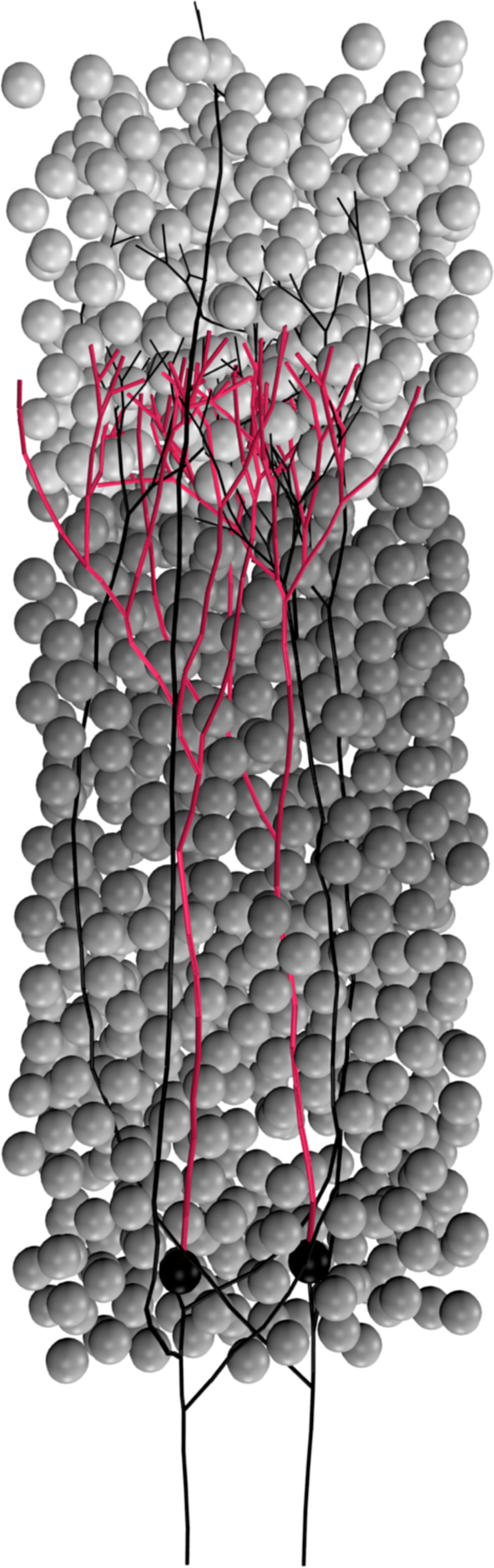
Figure 1. Typical CX3D simulation. The figure shows the result of a simulation in which two neurons extend dendritic (red) and axonal (black) arbors in a dense cortical column, according to the model specification described in Figure 7
. The physics engine prevents a branch from passing through another cell. (Half of the cells in the column were removed for better visualization). The 3D rendering was obtain by exporting the result of the CX3D simulation into the free program Blender (http://www.blender.org
). The mesh used for the rendering was created with the free java-based software ImageJ3DViewer (http://www.neurofly.de/ImageJ3DViewer
).
To define this neighborhood relation we use a 3D Delaunay triangulation (Schaller and Meyer-Hermann, 2004
). Given a set P of points in 2D, a triangulation T is a collection of non-overlapping triangles whose vertices coincide with the members of P, that covers the convex hull formed by P. The points and the edges of the triangle define a graph structure. Two points are defined as neighbors if and only if there is at least one triangle t ∈ T of which both are a vertex, i.e. if they share a common edge in the graph. The Delaunay triangulation is a special triangulation, defined by the condition that no point of P is inside the circumsphere of any triangle of T. In 3D, the method generalizes to the Delaunay tetrahedralization, where a set of points in space defines a set of tetrahedrons (for simplicity, we will nevertheless use the term triangulation even in the 3D case). In our framework, each discrete object is associated with a vertex in a 3D triangulation. CX3D uses the package Dyna3D written by Goehlsdorf
1
.
If the cell density is very low, it might happen that two physical objects far apart are considered as being neighbors, just because there is no other object between them. In this situation, for computational reasons, the user might want to add additional ‘empty’ vertices to the triangulation, so that physical interactions between pairs of remote objects are not evaluated (Figures 2
A,B).
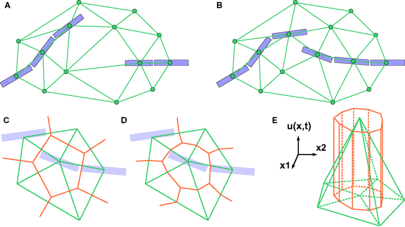
Figure 2. 2D illustration of the Delaunay triangulation and its dual graphs. (A) Each discrete physical object (blue) in the simulation is linked to a vertex in the Delaunay triangulation (green). Additional vertices represent empty regions of space. Two objects are considered as being neighbors when their vertices are linked by an edge. (B) When existing objects move or are deleted, or when new objects are created, their associated Delaunay vertex is automatically moved, deleted or inserted, and the triangulation locally updated. (C) The Voronoi graph (orange) is an example of a dual graph used to define a vertex-centered volume decomposition based on the Delaunay triangulation. The volume around each vertex contains every point in space that is closer to this vertex than to any other. (D) Another dual graph: the median dual graph is the set of lines joining the centroids (or barycenters) of all edges and triangles adjacent to a vertex (in 3D: all the edges, triangular faces and tetrahedrons adjacent to a vertex). (E) In the finite volumes method, for a given substance, only the average concentration ui(t) over a domain Vi is known. The total quantity Qi(t) of the substance inside the domain is equal to ui(t) Vi (the volume of the orange column). If the domain is defined by the median dual graph, a linear vertex-centered function with peak of ui contains exactly the same quantity (volume of the green pyramid). This representation is extremely convenient when we have to interpolate the concentration outside the vertices.
Diffusion processes
For the simulation of diffusion, we use an approach similar to the finite volume method (Barth and Ohlberger, 2004
). The extracellular space is decomposed into small non overlapping domains. When a physical object secretes a certain quantity of a signaling substance, the concentration of this substance increases in the domain containing this object. Let i and j be two compartments with respective volume Vi and Vj, containing the amount Qi and Qj of a given substance (hence the concentrations are ui = Qi/Vi and uj = Qj/Vj). If they are in contact, Fick’s first law tells us that the net flux Ji→j (in units of quantity per time) going from i to j is:
where D is the diffusion coefficient of the substance, Sij the area of contact between the compartments and dij the distance between their centers.
A first approach would be to multiply the flux Ji→j by the simulation time step Δt to compute the quantity transfered from i to j during the time step, to subtract it from Qi and add it to Qj. The new concentrations could be found by dividing the new quantities by the respective volumes. Using this formula in our simulation is equivalent to the Euler explicit method. But it comes with a very high risk of overshoot if the time steps are too large, especially in our case with an irregular decomposition of space. It is thus preferable to solve analytically the diffusion between each pair of neighbors: Remembering that Qx and ux vary with time, we obtain the following ordinary differential equation:
To get rid of the dependence on the quantity in the compartment j, we define the total amount T = Qi + Qj that is time-invariant. We can now solve the equation above and obtain:

with  and the integration constant
and the integration constant The median dual graph
The Delaunay triangulation that we use for near-object detection already provides us with a decomposition of space in discrete volumes (the tetrahedrons). But since all substances are produced and probed at the vertices of the triangulation (where the cell elements are located), it makes sense to use a dual graph, i.e. another decomposition containing the Delaunay nodes in the center of its volumes. The most popular graph with this property is the Voronoi graph (Figure 2
C), but for computational reasons we use the median dual graph (Figure 2
D). Firstly because it is not necessary to compute the boundaries of a domain to compute its volume (it’s simply one-fourth of the volume of the adjacent tetrahedrons). Secondly, because if we consider that the average concentration ui(t) for domain i given by the finite volumes method corresponds to the real concentration at the vertex position, and that we use linear interpolation between the vertices to define the concentration elsewhere, we get a better numerical approximation with the median dual graph (Figure 2
E).
To define the gradient on the Delaunay vertices, we recall that the directional derivative of the concentration u at the point xi along the unitary vector ê is equal to the dot product of ê with the gradient of u at xi:

We can approximate the directional derivative at xi along a vector pointing to any neighbor vertex xj by taking the difference of the two concentrations divided by the distance between them. With three different xj, we obtain a system of three equations that we solve to find the three components of the gradient at xi:

The smaller the volumes of the dual graph are, the better the precision of the diffusion simulation. This is another justification for having additional vertices added to the Delaunay graph even in absence of physical objects at that location.
Figure 3
A shows a test system introduced to illustrate the performance of our simulator on various aspects of diffusion. It consists of 500 vertices randomly distributed into a 200 × 200 × 200 μm3 cubic volume. The points are triangulated, with the median dual graph defining 500 volumes surrounding the vertices. Inside each discrete volume, we place a precise quantity of three diffusible substances in order to get a desired concentration, varying with the position of the vertex along one spatial dimension: The concentration profile of chemical R (red) is a step function, of G (green) a linear function and of B (blue) a cosine. Figures 3
B,C show the evolution of the concentration profiles over time due to diffusion.
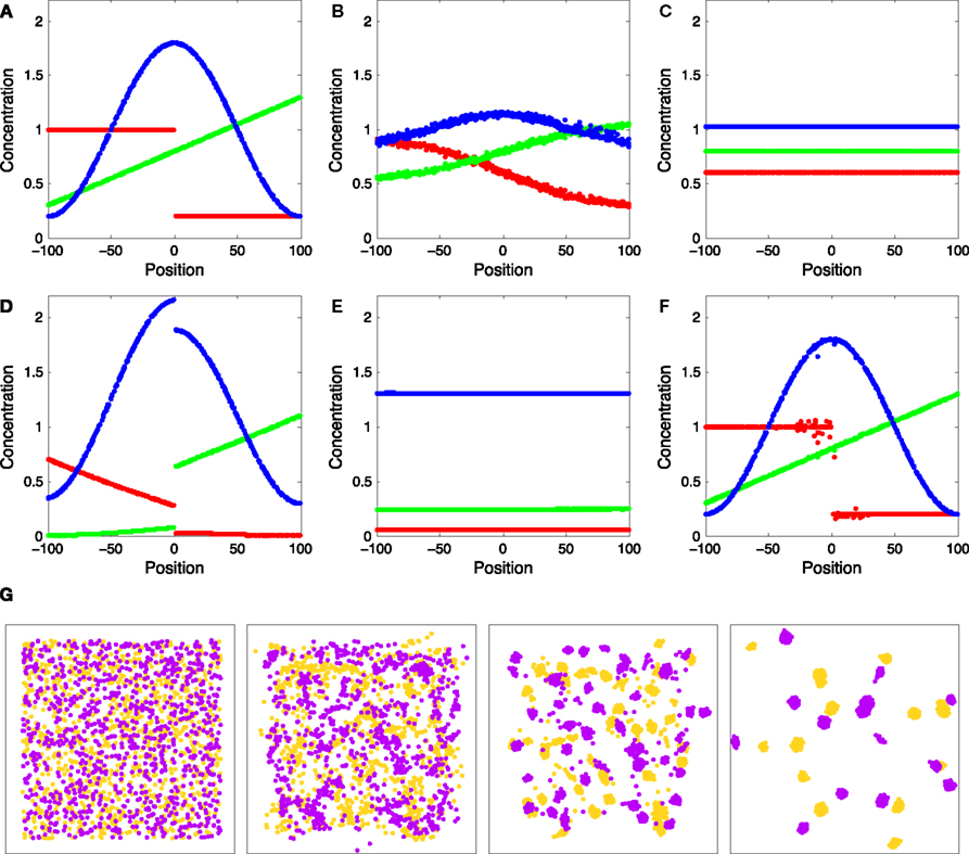
Figure 3. Test system for diffusion and chemical reactions. (A) Initial chemical concentrations in the discrete volumes created by the triangulation of 500 vertices randomly placed inside a cube. The concentration of three substances define a particular profile, dependent on the volume’s central vertex location along the horizontal axis (red substance: step concentration profile; green substance: linear profile; blue substance: cosine profile). (B) Evolution of the concentration profiles due to diffusion after 50 simulation time steps. (C) Concentration profiles after 500 simulation time steps. (D) Concentration profiles after 500 simulation time steps due to the chemical reaction  (see text), without diffusion. (E) Concentration profile after 500 steps of the same chemical reaction with diffusion included. Compare with diffusion without reaction in (C). (F) Minor alteration in the concentration profiles after 100 sequences of movements of three central vertices, without diffusion or reaction. (G) Use of diffusion in simulation: 1000 yellow cells and 1000 violet cells, secreting respectively ‘yellow’ and ‘violet’ diffusible cues, are distributed randomly in a 3D volume. They aggregate by following the gradient of their cell-type specific cue (results after 0, 300, 800 and 6000 time steps).
(see text), without diffusion. (E) Concentration profile after 500 steps of the same chemical reaction with diffusion included. Compare with diffusion without reaction in (C). (F) Minor alteration in the concentration profiles after 100 sequences of movements of three central vertices, without diffusion or reaction. (G) Use of diffusion in simulation: 1000 yellow cells and 1000 violet cells, secreting respectively ‘yellow’ and ‘violet’ diffusible cues, are distributed randomly in a 3D volume. They aggregate by following the gradient of their cell-type specific cue (results after 0, 300, 800 and 6000 time steps).Chemical reactions
In addition to diffusion and secretion by cells, the substances in the extracellular space are subject to concentration changes due to degradation and possibly other chemical reactions. Degradation is processed together with diffusion (a diffusion and a degradation constant can be specified for each extracellular substance). To introduce chemical reactions, the user has the possibility to define changes of concentrations that are applied at each time step on each discrete volume of the extracellular space.
As an illustration, we implemented in our test system the reaction  (with k1 = 10 and k−1 = 0.5), which corresponds to the combination of one molecule of the red and one molecule of the green substance forming one molecule of the blue substance, by applying the following concentration changes in each volume at each time step:
(with k1 = 10 and k−1 = 0.5), which corresponds to the combination of one molecule of the red and one molecule of the green substance forming one molecule of the blue substance, by applying the following concentration changes in each volume at each time step:
Figures 3
D,E show the result without and with concurrent diffusion respectively.
Influence of grid deformations on the concentration profile
Modifications of the Delaunay mesh have dramatic effects on the dual graph that we use to numerically solve diffusion. Thus we needed to incorporate a mechanism to automatically redistribute the different quantities of substances after each operation on the triangulation (physical object displacement, duplication or removal). The two major requirements are to preserve the concentration profiles, and to ensure mass conservation. Consider the case where the Delaunay vertex at position xi moves. If we didn’t update the quantity of substance located inside the surrounding volume, moving the point would result in substance transport. Our update mechanism consists of two phases: first we interpolate the concentration u′i of the chemical at the new location x′i of the moving vertex, and modify the quantity in the newly formed volume V′i to obtain this desired concentration, i.e. define new Q′i so that Q′i/V′i = u′i. Then we compensate for total mass conservation by multiplying the concentrations and the quantities in the surrounding volumes by the ratio between the total quantities before and after the displacement. Similar update mechanisms are used for vertex insertion or removal.
The procedure is tested in our bench test by moving three inner vertices 100 times (Figure 3
F). The displacement is a random 3D vector of less than 5 μm, with a re-centering mechanism to ensure that the points stay inside the convex hull of all other points. This minimally disruptive procedure allows for gradient ascent even in the extreme case where all physical objects are moving (Figure 3
G).
Mechanical Properties of Neurons
The complex shape of neurons, composed of dendritic and axonal arbors, makes the computation of their mechanical properties and interactions a difficult task. Following a technique that is used commonly in mechanical engineering and virtual reality contexts (Ng and Grimsdale, 1996
; Ward et al., 2007
), neurons in CX3D are composed of chains of springs and masses in series to provide structural integrity and propagate tension. Spherical and cylindrical wrappers enclose the spring-mass chain to confer volume on the cell and define spatial interactions between neighboring objects. Each wrapper is an independent object containing a single point mass. At each time step, it computes the local forces on its point mass and moves it accordingly.
Somata are defined by a sphere with a central point mass, whereas neurites are composed of cylinders, each containing one spring and one point mass at its distal end (Figure 4
). The disadvantage of this configuration is the asymmetry of the cylinders. The substantial advantage, on the other hand, is that we can neglect rotations of cylinders. Indeed each one is responsible for moving only its distal end (where the point mass is located), whereas its proximal end is defined by the position of its attachment point on the proximal discrete object. During neurite extension, some cylindrical elements are elongated. If their length exceeds a specified threshold, they split into two elements. Similarly, in case of retraction, short cylinders fuse. By this mechanism we ensure the suitable discretization of the cell. This discretization also permits intracellular diffusion. The simulation is performed in a similar way as for extracellular diffusion, but the volumes are defined by the cylinders and the sphere composing the neuron, and substances flow along the chains of elements regardless of the triangulation or its dual graph.
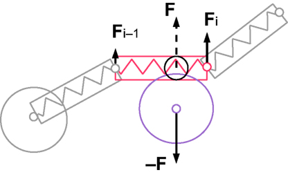
Figure 4. Cartoon representation of the physical discretization and inter-object mechanical forces in CX3D. Neurons are discretized into small physical objects, composed of a single point mass and a spherical (for the cell body) or cylindrical (for the neurite elements) envelope. The envelopes are used to define inter-object forces when two objects come into close contact. In this example, a cylinder in a neurite (red) and the sphere of an other cell’s soma (violet) overlap, which triggers opposite repulsive forces (F and −F). To determine the repulsion intensity, we define a virtual sphere (black circle) on the cylinder. The forces are proportional to the overlap of the virtual sphere and the soma sphere. Spheres have a central point mass, and the force is directly applied on it. Cylinders have their point mass at the distal extremity, so only a fraction of their inter-object force is applied on it (Fi), while the rest is transmitted to the proximal element’s point mass (Fi − 1). In addition, cylindrical elements contain a spring which is always attached to another proximal element, and propagates tension along the chain of point masses.
Forces
Three different types of forces can be applied to each point mass. The first type arises from the interaction between the physical objects when they come into close contact. The second type is the internal tension arising when a neurite is stretched, which is modeled by the springs connecting the masses. This internal tension both influences, and is influenced by, metabolic growth. The third type of forces represents the active movement of cell elements. It follows from the biological properties of the model specified by the user.
Inter-object forces
Cells in a tissue have strong resistance to compression. They also have adhesive properties. Consequently they are conveniently modeled as a granular medium with additional bindings (Schaller and Meyer-Hermann, 2005
; Shinbrot, 2006
). The physical interaction between two spherical somata is then a function of their diameter, their relative distance, and possibly their expression of adherence molecules.
It is possible for users of CX3D to define their own cell–cell interaction function. However, by default a modified version of (Pattana, 2006
) is used, in which the force from sphere si onto sphere sj contains a repulsive component (preventing two cells to overlap) and an attractive component (representing the integrity of the tissue and forces resulting from cell adhesion molecules):
where k is the repulsion coefficient, γ the attraction coefficient, ri, rj the radii of the spheres, δ the overlap: max(0,ri + rj − distij), and ê the unitary vector pointing from the center of sphere i in direction of sphere j.
The radius ri used in the previous equation needs not to be exactly the radius of the sphere si. For instance, to reproduce the different neuron densities observed one can use larger effective radii, which increases the range of interaction and hence pushes cells further apart from each other. Or one can use smaller radii for migrating cells, and thereby model the possible deformations of moving cells that are less perturbed by the surrounding tissue.
In CX3D, we must also consider cylindrical objects, which means that there are in fact three different sorts of interactions: sphere–sphere, sphere–cylinder and cylinder–cylinder. For instance, to compute the interaction between a sphere s1 and a cylinder c, we define on c a virtual sphere s2, and then compute the interaction between the two spheres s1 and s2 as described above.
Cylinders have their unique point mass located at their distal end. So, if the inter-object forces applied to a particular cylinder only affect its own point mass, it means that only one of its extremities will ever move. Therefore, part of this force has to be transmitted to its proximal segment (i.e. the object responsible for the mass situated at the proximal end of the cylinder). This repartition of forces along chains of cylinders is essential for stability.
In addition to the attractive component of the inter-object interaction, additional specific adhesive bonds, permanent or transient, can be added between neighboring objects. These links consist of additional springs between two discrete physical objects. Such links can be used, for example, to stabilize the pre- and post-synaptic cell elements with respect to one another at the location of a synapse.
Intracellular tension
Dennerll et al. (1989)
have reported that neurites show passive viscoelastic properties when stretched with a force smaller than 1 nN. During the 10 first minutes they observed two passive phases: a rapid increase in length and tension, followed by a damped phase. Mechanical models with a spring and a Voigt element (spring and dashpot in parallel) or a Burger element fit these data well. If a larger force is applied for a longer time, a third phase is observed in which the neurite continues to extend while the tension diminishes, sometimes to less than the tension before the application of the perturbing force. This third phase corresponds to active growth, including reorganization of the cytoskeleton and incorporation of membrane components. This phenomenon explains ‘towed growth’ (growth not generated by the growth cone).
Our model does not differentiate between the two passive phases, since we consider only springs in series, which is a reasonable approximation to neurite passive mechanical properties (Dennerll et al., 1988
). The absence of a dashpot is compensated for by the use of the overdamped approximation in the equation for movement (see below). The tension vector due to the internal spring in a cylinder is thus:

where k is the linear spring constant of the neurite, aL the actual length of the spring (length of the cylinder), rL the resting length of the spring and ê the unitary vector aligned with the central line of the cylinder.
The metabolic phase is modeled by changing the resting length of the springs; for instance, rL → rL + ΔL for elongation, which automatically decreases the tension. As described above, the number of discrete cylinders scales with the length of the neurites. The discretization mechanism is based on the resting length: if it exceeds a certain threshold, the cylinder is split into two, each half retaining the same tension.
Active displacement
The biological properties specified by users often require the active movement of spheres and of neurites’ terminal cylinders, for instance in the case of cell migration or neurite extension. In this case, an additional force is applied to the physical objects’ point mass. The moving objects do not modify their trajectories ahead of time in case of an upcoming collision. But if after the displacement two objects have come too close (or interpenetrate), a repulsive force is triggered between them. This system is as stable as trajectory interpolation, but is less computationally demanding.
In the case of neurite extension, the displacement of the distal point mass must result in an increase in the resting length of the corresponding spring (as in towed growth). It has been shown (Lamoureux et al., 1989
) that the extension rate of an axon is proportional to the tension its growth cone is applying, in the following sequence: movement → stretching (increase in actual length) → increase in tension → active growth (increase in resting length). Although we could reproduce this sequence in CX3D, for computational reasons we usually take a short cut: First the growth cone is moved and then the resting length is set in order to obtain the desired tension. Similar mechanisms are possible for retraction: A reduction of the resting length will induce an increase in tension and then a backward movement of the distal point mass. Alternatively, the point mass can be moved first, and then the resting length is updated to maintain the desired tension.
Movement
During the simulation, each discrete physical object evaluates all instances of the three forces applied to it, and sums them to obtain the total force acting on it. If the total force exceeds a certain threshold, the object moves its point mass appropriately (Figure 5
). For instance, the cylinder i checks if any neighbor in the triangulation is exerting a force Fij on it, including possible adhesive bonds b. It also takes into account the tension in its internal spring (Ti) and in the springs of the daughter cylinders directly attached distally to it, if any (note that a terminal cylinder has no daughters, a cylinder in a chain has one daughter and a cylinder proximal to a branching point has two daughters).Finally, it might also have some biological movement M to take into account:
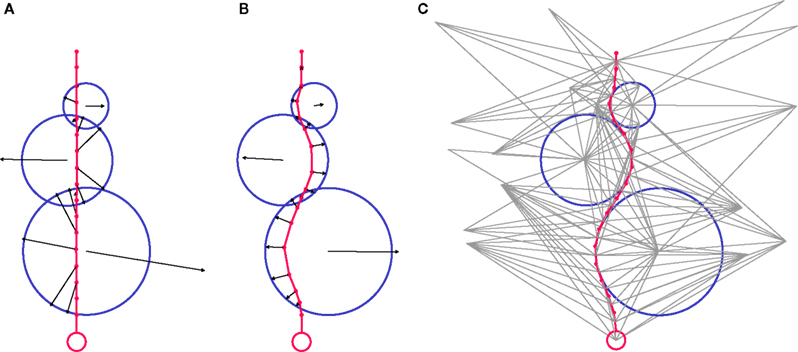
Figure 5. CX3D simulation snapshots demonstrating the mechanical interactions in a test system, composed of a chain of cylinders attached to a small sphere (red), and three bigger spheres (blue). The total force applied to each point mass is represented by a black arrow. (A) We start with the artificial situation where the chain of cylinders and the three spheres are strongly overlapping. This condition triggers a radial force on each of the cylinders’ point masses, pushing them outside the spheres. The spheres are subject to the sum of the opposite forces, plus the sphere–sphere interactions. (B) After the system has started to relax due to objects being displaced, the magnitudes of the forces start to diminish. The radial movement of the cylinder point masses has resulted in an elongation of the internal springs joining them, which triggers an intra-object force that adds to the component due to the object overlap, and hence results in a less radial total force on the cylinders. (C) After complete relaxation, there is no object overlap anymore, and the distances between the point masses of the cylinders chain correspond to the springs resting lengths. Therefore there is no force present anymore. For each discrete object in the system, the link to its neighbors, defined by the 3D Delaunay triangulation is shown (grey). Note the additional vertices that are not corresponding to a physical object.
In classical mechanics, the equation for movement in a medium with friction is

where  is the acceleration,
  the speed, m the mass and β the kinetic friction. Neuron elements in a tissue have a low Reynolds number (typically 10−7 for a growth cone; Aeschlimann, 2000
), which means that the ratio of the inertial forces to the viscous forces is low. It is then perfectly reasonable to make the overdamped approximation: That is, to assume
the speed, m the mass and β the kinetic friction. Neuron elements in a tissue have a low Reynolds number (typically 10−7 for a growth cone; Aeschlimann, 2000
), which means that the ratio of the inertial forces to the viscous forces is low. It is then perfectly reasonable to make the overdamped approximation: That is, to assume  The consequences of this assumption are (1) that an element doesn’t move if it is not currently subject to a force and (2) that the major obstacle to movement is no longer the mass but the friction coefficient. Consequently, physical objects in CX3D move according to:
is the acceleration, the speed, m the mass and β the kinetic friction. Neuron elements in a tissue have a low Reynolds number (typically 10−7 for a growth cone; Aeschlimann, 2000
), which means that the ratio of the inertial forces to the viscous forces is low. It is then perfectly reasonable to make the overdamped approximation: That is, to assume The consequences of this assumption are (1) that an element doesn’t move if it is not currently subject to a force and (2) that the major obstacle to movement is no longer the mass but the friction coefficient. Consequently, physical objects in CX3D move according to:
In addition, we have a term for static friction that provides a threshold for the initiation of movement. If the total force exceeds the static friction, then the actual movement is computed using the explicit Euler method: Multiplying the speed with the time step to obtain the actual displacement:
Implementation
CX3D is written in Java because it is an object-oriented language; it benefits from many libraries (for visualization for instance); it does not have to be recompiled to run on different platforms; and it provides methods for distributing processes across multiple computers, which will be crucial for future development.
Our software design is modular, keeping a clear separation between the biological processes on the one hand, and the infrastructure needed to run the physics and computationally organize the simulation on the other hand. Four abstract layers are used in the representation of cells (Figures 6
A,B and Appendix). In addition, CX3D contains several utility packages that are not discussed in this paper.
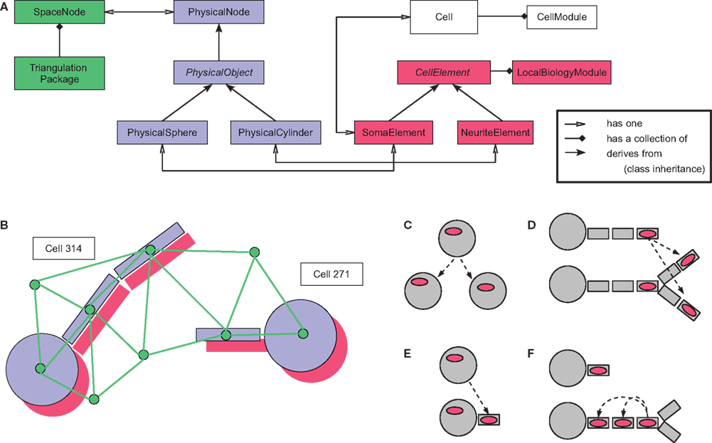
Figure 6. Program architecture of CX3D. (A) Java class diagram and
(B) cartoon representation of the four abstract layers used in the representation of a cell in the CX3D framework: the Delaunay triangulation defining a neighborhood relation between space regions and physical objects (green); the physical layer containing the classes representing the discrete space regions and the physical objects contained in them (blue); the local biology layer, with biological elements associated with the physical objects (red), and finally the higher level biological properties expressed at the cell level (white). See Appendix for a detailed description of the java classes. (C–F) Local biology modules specifying the simulation properties are associated with specific cell elements. When new objects are created, the local biology modules can be automatically copied according to four different schemes: when cells divide, when neurite elements branch, when new neurites are being formed from the soma, and during neurite elongation.
To design a particular cellular model, users must write modules (small java classes implementing a special interface) that are inserted into the cells to engender their specific functionality. There are two different types of modules: Local biology modules; and cell modules.
Local biology modules represent all the local biological processes. Each one is attached to a particular physical object (one of the spheres or cylinders used to represent the neuron) and reads from it physical data such as current volume, tension, or concentration of an extracellular substance. Likewise, the module sends instructions to the physical object, for example to move, change its shape, or to extend a new branch. For instance, the simplest module for performing chemotaxis would repeatedly execute the following three steps: (1) query from the associated physical object the gradient of an extracellular substance’s concentration, (2) compute a desired movement, (3) transmit a movement direction and speed to the physical object. CX3D would perform the displacement, update the physical values (e.g. define a new length in the case of a cylinder), and update the triangulation. If the movement had brought the object too close to another physical object, a symmetrical force will be applied on both objects at the next time step, possibly pushing them away from one another again. Local biology modules can be copied automatically into new discrete cell elements in case of soma division, new neurite extension, neurite branching, or neurite elongation (Figures 6
C–F).
Cell modules are used to model biological processes affecting the whole cell, such as cell cycles, or gene expression. Because they characterize the entire cell, these modules cannot be linked to any particular spatially located spheres or cylinders that represent the spatial discretization of the cell.
CX3D provides a general framework for various types of neural growth simulations. In this section we present five examples of different kinds of problems that could be simulated with CX3D. Each example was obtained by writing appropriate local biology modules and cell modules that provide the biological functionality required for each case. The first three examples are original models, and the final two are previously published models now re-implemented in CX3D.
Formation of a Layered Cortex
Our first example models the formation of a layered cortical-like structure (Figure 7 and Videos S1 and S2 in Supplementary Material). During corticogenesis, neuron precursors are generated by division of the progenitor cells in the ventricular and subventricular zone (Kriegstein and Noctor, 2004
). These precursors then migrate radially, climbing along long processes attached to the radial glial cells (Rakic, 1972
), from which they detach before entering the cells that will form the future layer 1 (L1). It is remarkable that each generation of neurons migrates through all its predecessors, leading to an inside out formation of the cortex, with first cells of layer six (L6), then five (L5), four (L4) and finally three and two (here considered together as L2/3). L1 cells are continuously pushed further away from the ventricular zone. The exact control mechanisms for the detachment is not clear, but the protein reelin, produced by some L1 cells is necessary. We simulated a model in which reelin is the only signal present (Cooper, 2008
).
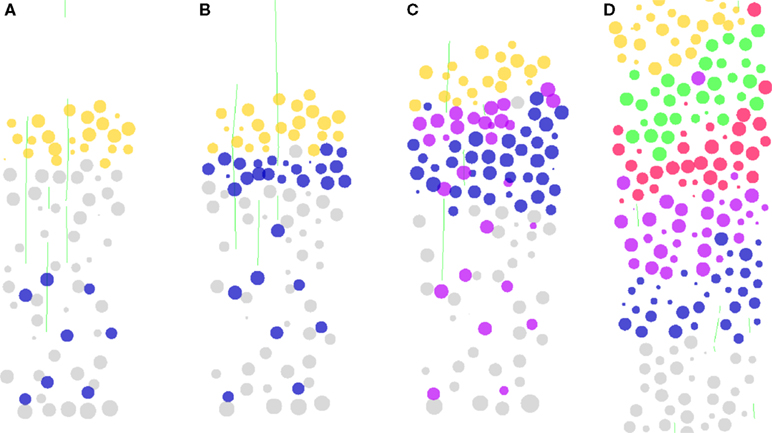
Figure 7. Simulation of cortical layers formation. The figure shows a section through a volume of developing tissue. (A) Layer 6 neuron precursors (blue) are produced by asymmetrical division of the progenitor cells (larger grey, at the bottom). They migrate along radial glial processes (green fibers). (B) Once the neuron precursors detect a contact with the top-most L1 cells (orange), they stop their migration by detaching from the radial fibers. Due to the mechanical interactions between cells, the first layer is pushed upward. (C) When L5 neurons are produced, they follow the same path, passing through L6 cells until they contact L1. (D) Similarly with L4 and L2/3. Each generation passes through all the predecessors, to form a layered structure. Due to the large mechanical forces, a few cells in this simulation end up in the wrong layer, as observed in the cortex (Polleux et al., 2001
).
The simulation is initialized with an array of 8 by 8 radial glial cells, each having a long process that extends vertically through a volume of preplate cells (subplate cells and future layer one cells on the top). These glial cells divide asymmetrically and form neuronal precursors. Depending on time, they form first L6 cells, then L5, L4 and L2/3 (colored in blue, violet, red and green respectively). The neuron precursors have inside their local biological modules the instructions to execute the following sequence: (1) To move randomly until they touch a radial fiber on which they fix themselves. (2) To migrate (distally) along the radial fiber. (3) To leave the fiber when they encounter an L1 cell, and thus stop their migration. Due to the physical properties of the spheres, the neuron precursors split the preplate and push the L1 cells, so progressively displacing the stopping signal. The fact that we can reproduce the inside-out lamination of the cortex with this extremely simple set of instructions highlights the importance of incorporating mechanical interactions in the simulation of developmental processes.
Layer Specific Dendritic Growth
The second example (Figures 1 and 8 and Video S3 in Supplementary Material) illustrates the use of diffusible guidance molecules and how they can be used to produce layer-specific branching patterns of neurites (Castellani and Bolz, 1997
; Dantzker and Callaway, 1998
). The simulation begins with an already-formed three layer cortex that could have been produced by mechanisms similar to those of the previous example. The layers are formed of three different types of cells (L6, L5 and L4), all secreting a diffusible, layer-specific substance (for instance each L4 soma produces only the ‘L4’ substance, etc.). These substances diffuse through the environment, establishing chemical gradients that will guide the development of the axonal and dendritic neurites from two test cells inserted in L6, leading to a branching pattern that respects the layer specificity of pyramidal cells of layer 6. Namely, a down-going main axonal shaft, which produces side branches in L6 that move up to L4, where they ramify, and an apical dendrite, also terminating in L4, but starting to branch earlier than the axons.
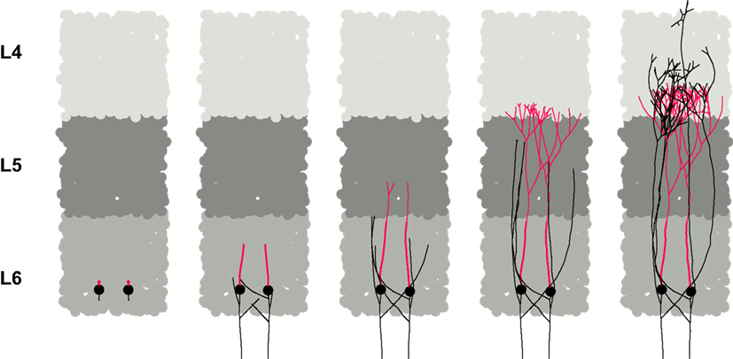
Figure 8. Branching pattern based on extracellular signaling molecules. In this simulation, we started with a column of a cortex-like tissue, with three layers composed of specific cell types (L6, L5 and L4, depicted in medium, dark and light grey respectively). Each cell secretes a layer-specific diffusible chemical, serving as guidance cue for the layer specific growth of the axonal and dendritic arbor of two test cells. The usual layer preference of typical L6 pyramidal branch could be reproduced: an apical dendrite (red) branching at the L5-L4 transition, and a down-going axon (black), with side branches in L6, moving up to ramify in L4.
In this simulation, each cell type forming the layers contains a single module, responsible for secreting the appropriate substance. The diffusion is performed automatically by the physics engine of CX3D. For the development of the branches, we wrote two small modules modeling the growth-cone functions and inserted them into the initial neurites. One of the modules elongates its neurite by moving its cylinder point mass either down the gradient of the L5 substance (for the axonal main trunk) or up the gradient of the L4 substance (for all other branches). The other module allows branching to occur with a probability that depends on the local concentration of a specific substance (L6 for the initial axon, L4 for the others branches). Different concentration thresholds for branching have been defined for the axons and the dendrites, and therefore the latter start their ramification earlier. Both modules are copied at branch points into the two new daughter growth cones. Neurite diameters decrease during elongation and at branch points, and the growth stops when the diameter has become smaller than a certain threshold.
The purpose of this simulation was not to reproduce exactly the morphological properties of specific cell types, but rather to illustrate the importance of long range inter-cellular communication through secretion and detection of diffusible cues.
Dissociated Culture
Much can be learned from dissociated cell cultures, because their architecture is simpler than cells developing in-vivo, and because they are more accessible to imaging technics. Also, by growing cells on multiple electrode arrays it becomes possible to selectively record from, and to simulate, elements of a network. Some research groups have been interested in modeling this neuron–silicon interface, and have made growth simulations of neurons on a plate (Massobrio et al., 2007
).
By restricting the cell movements to a very thin section of space, we can reproduce the 2.5D environment of cell cultures on a Petri dish. Our next simulation (Figure 9
A and Video S4 in Supplementary Material) shows 12 isolated cells on a plate, extending an axon and several dendrites. As in the previous example, each terminal neurite element contains a movement module and a branching module responsible for the extension of the cells. The main difference is that no guidance molecules are produced, so leading to the formation of an isotropic network.
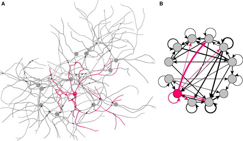
Figure 9. Dissociated culture neurons forming a network. (A) Eleven excitatory (grey) and one inhibitory (red) cells are randomly disposed in a 2.5D environment. They extend 4–7 neurites; one of them, thinner and growing faster, represents the axon. An attractive force between the cell elements induces a tendency to fasciculate. After the growth is completed, synaptic connections are formed randomly between neighboring axons and dendrites (black links). (B) Graph representation of the circuit shown on the left, drawn from a NeuroML description of the network, exported from CX3D after the simulation (black arrows: excitatory projections; red arrows: inhibitory projections; line thickness proportional to the number of synapses between cells).
This example illustrates two other features of CX3D. First, the possibility to change the cell–cell physical force. In this example, by increasing the range and the strength of attraction in the interaction between cylinders, we reproduce the fasciculation of neurites often observed in cultures. Secondly, the formation of a neuronal network: If an axonal neurite element comes into close contact with a dendritic neurite element, a synapse is formed with a certain probability between the two elements (Stepanyants et al., 2002
). Neurons and their connections define a network (Figure 9
B), whose description can be exported as an XML document that conforms to the NeuroML (Goddard et al., 2001
) description used for specifying electrophysiological simulations. This bridge from developmental to electrophysiological simulation offers a valuable tool for scientists interested in studying electrical activity in developing networks. Of course, it would be possible in future to extend CX3D to provide direct simulation of electrophysiology.
Contact Inhibition
Lateral inhibition is an important mechanism for selecting – in an homogeneous population – individual cells that will adopt specific characteristics. One of the most studied pathway involves the transmembrane proteins Delta and Notch, from which Collier et al. (1996)
published a model: Notch is activated by the expression of Delta on the neighboring cells, whereas Delta is inhibited by the Notch level on the same cell. Additionally, both proteins are subject to exponential decay. This gives rise of a pattern of cells with a low Notch and high Delta profile, surrounded by cells with high Notch expression.
Collier et al. (1996)
were mainly inspired by observations on Drosophila, but the Delta-Notch system is commonly found throughout neural systems development, including in the mammalian cortex where it is used to determinate which cells will acquire a neuronal or a glial fate. Therefore, we took it as a test example of how other models can be re-implemented in our framework. By doing so, the model originally developed on a 2D regular grid could be extended to a 3D agent-based version (Figure 10
). In addition, now that it is coded in CX3D, it can be combined with other models in larger simulations. For instance to select the cells that will divide in a tissue (Video S5 in Supplementary Material).
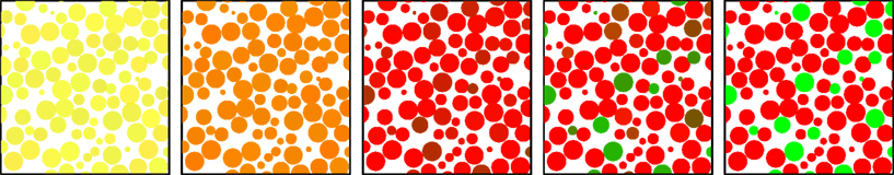
Figure 10. Simulation of pattern formation by lateral inhibition (surface molecules). The simulation starts with a homogeneous population of cells expressing equal concentrations of the membrane bound ligand Delta (D) and its receptor Notch (N). According to the model of (Collier et al., 1996
), each cell activates over time N in the neighboring cells, depending on its own D level, while decreasing its own D concentration based on its N level. The result is the selection by lateral inhibition of cells with a low N and high D. Such cells are not contiguous. (Red color intensity proportional to N, green proportional to D. Equal level of red and green intensity appears yellow).
Cell elements in CX3D can express membrane-bound substances. We designed a local biological module to regulate the expression for Delta (D) and Notch (N), according to the following dynamics:
with f(x) = min(1,20x), g(x) = max(0,1 − x) and  is the average value of Delta on all the cells in close contact. This example is another illustration of the importance of modeling physics in a general purpose simulator (here to detect contact between close neighbors).
is the average value of Delta on all the cells in close contact. This example is another illustration of the importance of modeling physics in a general purpose simulator (here to detect contact between close neighbors).Internal Resource Competition
For this last example, we demonstrate the implementation in CX3D of a previously published model of neurite outgrowth. Kiddie et al. (2005)
presented a 2D model based on a production-consumption mechanism: the soma produces two substances, tubulin (T) and microtubule associated proteins (MAPs), which diffuse intracellularly to the distal branches of the neuron. T accounts for extension and retraction of growing neurites by polymerization and depolymerization of microtubules. MAPs, after transformation into several isoforms, regulate the branching probability by modifying microtubule stability.
To implement their model in CX3D (Figure 11
), we wrote an intracellular secretion module for the soma production of T and MAPs at a fixed rate, and a growth cone module which extends or retracts based on the local concentration of T, and bifurcates with a probability depending on the concentration of MAPs. The growth cone module is copied at each branching point. The intracellular diffusion is processed automatically by the physics engine of CX3D.
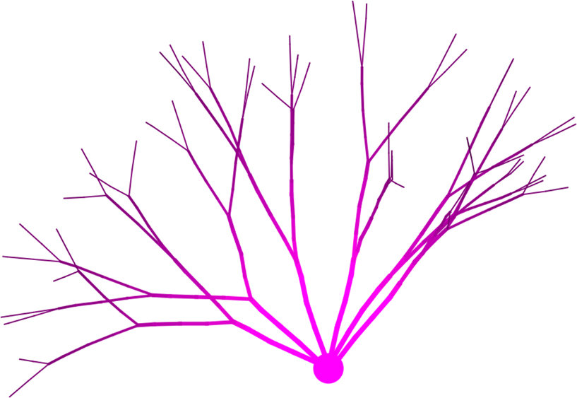
Figure 11. Simulation of branching pattern based on intracellular protein concentrations. The figure shows a 3D implementation in CX3D of the neurite outgrowth model of (Kiddie et al., 2005
). Tubulin is produced in the soma, diffuses internally and is consumed distally for branch elongation. The intracellular concentration is color coded (light pink: higher concentration). Additionally, microtubule associated proteins are also secreted at the soma, diffuse distally where they are transformed in several isoforms, regulating the branching behavior.
This last example was well-suited to the CX3D framework because it relies on local computation by independent agents (in this particular case each growth cone’s behavior depends exclusively on its intracellular concentration of T and MAP), and because it requires the modeling of physical processes (the intracellular diffusion).
Performance Testing
The execution speed of a CX3D simulation depends on the type of operations performed (in particular the proportion of physical objects that are moving). To test the performance of our framework, we present the CPU time required per time step for three different models. The simulation time step is 10−2 h, and the speed of actively moving cell components is uniformly set at 100 μm/h. All tests were performed on a MacBook Pro with a 2.4 GHz Intel Core 2 Duo processor, running Java 1.6.0.
The simulation of cell clustering shown in Figure 3
G is close to the worst case scenario, with each single physical object moving at each time step, and each cell element containing a local biology module. For 2000 cells and 400 additional triangulation vertices (i.e. 2000 PhysicalObjects, LocalBiologyModules, CellElements and Cells, and two substances diffusing across 2400 extracellular volumes), the initialization, i.e. the creation of all objects with the initial triangulation was done in 3.3 s, and the simulation of one time step took 400 ms. The images taken at 300 and 800 time steps are obtained respectively after 2 and 5 min 20 s. It took much more time to have already formed clusters move and fusion into larger cells assemblies; the last image taken after 6000 time steps required 40 min of simulation.
The situation is much more favorable in our model of lateral inhibition, where objects don’t move (and thus the triangulation is not modified), and where the substances are membrane-bound and thus don’t diffuse in the extracellular space. For 2000 cells and no additional triangulation vertex, the simulation takes 63 ms per time step. The pattern presented in Figure 10
is complete after 400 time steps, i.e. 25 s.
Most simulations in practice correspond to intermediate cases, in which only a fraction of the physical objects are actively moving, as for instance in the model presented in Figure 8
. For 1800 static somata and 100 additional triangulation vertices, with three extracellular substances diffusing, the simulation takes initially 135 ms per time step (at an early stage where the growing cells are composed of 140 non-terminal cylinders plus nine terminal cylinders with local biology modules in total). It requires 285 ms per time step at a later stage where there are 840 non-terminal cylinders plus 585 terminal cylinders. The total simulation time was 85 s.
Current efforts in developmental neuroscience research focus on reductive characterization of specific biological processes, such as biochemical pathways or gene expression patterns. These studies are essential to understand the mechanisms of brain development. However, even in the most studied systems, it is often difficult to understand how the higher level process of brain development emerges from interactions between these lower level mechanisms. Simulation offers a means of studying these organizational processes (van Ooyen, 2003
). CX3D, with its physics engine, its multi-agency and modular architecture is well suited for exploring these issues in neural development. Users describe the simulation specifications by writing small mechanistic modules that are incorporated into the cells, defining the biological properties locally or at cell level. Using this approach, one can study growth and development in simulations of hundreds of cells.
In self constructing systems, the environment (including physical laws) plays an active role in constraining the local interactions between agents. For instance, our first original simulation (Figure 7
) showed how a very simple sequence of instructions could reproduce the inside-out migration pattern of cortical neurons; but the division and migration of neural precursors would have failed to produce a layered structure if the inter-cell physical interactions had not participated in displacing the L1 cells upward. This result shows that CX3D could also be used for simulating other situations where mechanical forces play a major role in nervous systems development, for instance the formation of the neural tube (Shinbrot, 2006
), or cortical folding. In the latter case, a simulation might help to distinguish between causes and consequences (see for instance the different hypotheses linking cortical folding to intra-areal connections or respective cell numbers in supra- and infra-granular layers in gyrii and sulcii; VanEssen, 1997
; Hilgetag and Barbas, 2006
; Kriegstein et al., 2006
).
In the model presented in Figure 8
, we could reproduce a layer-specific branching pattern, because the biological modules active in the terminal branches of the neurites could detect the diffusible signaling molecules produced by other cells. Associated with the possibility of expressing and detecting membrane substances, it offers the possibility to investigate by simulation a number of classical problems in developmental neuroscience, such as optical tectum map formation (Goodhill and Richards, 1999
; Willshaw, 2006
), midline crossing (Goodhill, 2003
), and, of course, more accurate models of cortical neuronal development.
These simulation methods demonstrate how morphology and function can arise out of implicit rules. For instance in our second example (Figure 8
), the desired shape of the adult neuron was not explicitly specified in the code. Instead, local decisions on whether to turn or to branch were taken independently in the growth cones, based on local chemical conditions, which lead to the final cell architecture. If the guidance cues had been secreted at different locations, or if they were absent, the resulting branching pattern would have been completely modified. Due to its modularity CX3D provides the ability to run the same biological models in different test environments, which is a valuable tool for a modeler interested in studying the relative importance of extrinsic and intrinsic factors. The model for a cortical cell can be tested in a cortex-like layered structure with several guidance cues, or in a sparse in vitro environment like the one of Figure 9
. This kind of approach is interesting, in that it provides the modeler with two sets of constraints on a single set of parameters in the growth cone module. The fact that similar simulations can be run with various parameters, or after having selectively de-activated specific functions is also of interest for the study of mutations. For instance, in a more elaborated model of cortical plate formation incorporating various signaling molecules, it will be possible to suppress their activity totally or partially, to try to reproduce well-known phenotypes (Assadi et al., 2003
; Herms et al., 2004
), or maybe even to predict new ones.
Our goal was to provide a general purpose simulation framework for the simulation of the physical development of neuronal networks. We showed how two models from the literature could easily be implemented in CX3D. Indeed, we could rely on the physics engine for technicalities like neighbor detection or diffusion, and did not have to code them anew. An obvious advantage in using the same framework for several types of simulations is that they can easily be combined in a larger simulation. As an illustration, we added a cell cycle to the Delta-Notch model of Collier et al. (1996)
(Video S5 in Supplementary Material).
Future Work
We have given several examples of how CX3D can be used to simulate growth of neurons in 3D space. Although we have the ability to generate synapses at contact points between neurons, these synapses are not functional, because our program does not yet incorporate electrophysiology. However, where the electrophysiology is requested, we provide the ability to export a description of a grown network as an XML document with the NeuroML level 3 specification
2
(Goddard et al., 2001
). These documents can be used to configure a simulation in a point neuron electrophysiology simulator such as PCSIM
3
(Pecevski et al., 2009
). Future versions of CX3D could include an electrophysiology module directly inside neurites. Alternatively, modules could implement an interface for online communication with a coexisting electrophysiology simulator. This feature would of course be of great interest, because of the direct influence of electrical activity on neurite outgrowth (Hutchins and Kalil, 2008
), or on interneuron migration (de Lima et al., 2009
); and in a later phase to study phenomena like synaptic competition (Turrigiano, 2008
) and learning (Butz et al., 2009
). A further limitation of the present version of CX3D is that it runs on a single processor, so limiting both the speed and the size of simulations. However, we are currently developing a parallel implementation.
Program Architecture
This section describes the general organization of the CX3D platform by introducing the principal classes of each package.
There are four abstract layers in the representation of a cell in CX3D (Figures 6
A,B). One purely technical with which the user never interacts, one representing the physics of the simulation, on which the user has to call some methods, and two layers with which the user interacts by writing small modules describing the model’s specifications. Each layer correspond to a distinct java package:
(1) ini.cx3d.spatialOrganization: this layer defines the Delaunay triangulation and median dual graph needed to spatially organize the elements of the simulation, and decompose the extracellular volume. We use the package
Dyna3D developed by Dennis Goehlsdorf
4
. Vertices are defined by the class SpaceNode, of which each discrete object or space volume has one instance.(2) ini.cx3d.physics: the second layer represents the physical processes, both of the extracellular matrix (extracellular diffusion) and of the neurons (mechanics and intracellular diffusion), for which we use instances of the
PhysicalSpace class, and sub-classes of the abstract PhysicalObject, respectively. To have the latter derived from the class defining the extra-cellular matrix volumes ensures that any object in the simulation, as soon as it is instantiated, automatically comes with a minimal definition of the space it occupies. To embody the neurons in the simulation framework we discretize them into small spheres (for the somata) and cylinders (for the neurite segments) with the classes PhysicalSphere and PhysicalCylinder. They contain the methods needed for the simulation of the mechanics and offer an interface for communication with the biological modules so that the physical shape of the neurons can be modified by growth, branching, retraction etc.(3) ini.cx3d.localBiology: the third layer specifies the local biological properties of the simulation, namely the behavior of the spheres and cylinders, with the classes
SomaElement and NeuriteElement respectively (both subclasses of the abstract LocalBiologyObject). Instances of these are always associated with a particular PhysicalObject. These instances contain modules written by the users to define the specific rules governing the behavior of each discrete object in the model he wants to simulate. These modules are classes that implement the LocalBiologyModule interface.(4) ini.cx3d.cell: the fourth and last layer defines the higher level biological processes, influencing the whole neuron. As for the local biology level, it is composed of modules that the user can write, implementing a special interface (
CellModule). These modules are contained in the class Cell, of which there is only one instance per neuron.Finally, the user should be familiar with the package ini.cx3d.Simulation, which contains two important classes:
ECM contains a list of all the objects currently active in the simulation (instances of the classes described above). This class is also used for adding supplementary vertices to the triangulation, to define chemicals or chemical reactions, and to add boundary conditions.Scheduler contains methods to execute the simulation. That means that it calls the run() method of each object. Consequently, the physical objects process diffusion, compute their mechanical interactions and move accordingly. The local biology objects and the cells run all their modules (and thus the models are executed). The triangulation, on the other hand, is not run by the scheduler but only updated in case of vertex displacement, removal or insertion. The first time that the scheduling methods are executed, a GUI window appears, and graphically displays the physical objects.A Commented Example
The usage of CX3D is described in a tutorial available on the CX3D website
5
. We briefly illustrate the programming interface by implementing a simplified version of the model presented in Figure 11
: The soma secretes the intracellular substance ‘tubulin’ which diffuses along the neurite branches. The neurite distal segments (the growth cones) consume tubulin to move at a speed proportional to its concentration, and bifurcate with a constant probability.
To encode this simulation, we write three short java classes: two modules (a java class implementing the nine methods of the
LocalBiologyModule interface, or extending the abstract class AbstractLocalBiologyModule), and one additional class to initialize the simulation.Recall that each module is located within a
CellElement. Instances of this first module will be located in a soma, where they secrete tubulin at a constant speed:
The second module represents the growth cone. There is one instance of this class in each terminal neurite compartment. It performs a smooth random walk (the direction is slightly perturbed after each step), with a speed depending on the concentration of tubulin, which is also consumed in proportion to the speed. In addition, the growth cones bifurcate occasionally, in which case copies of the module are inserted into the new daughter branches:
Now we can set up and run the simulation, i.e. write a class to (1) define the substance ‘tubulin’; (2) create a cell (quadruple
Cell-SomaElement-PhysicalSphere-SpaceNode); (3) with an initial neurite segment; (4) place the local biology modules; and (5) start the scheduler:
This model is extremely simplistic, but it already exhibits interesting properties: The elongation speed decreases with the number of terminal branches, but the bifurcation probability over time is constant, and so the distance between two branch points becomes shorter. In addition the tortuosity also increases as the speed decreases.
The authors declare that the research was conducted in the absence of any commercial or financial relationships that should be construed as a potential conflict of interest.
We thank Dennis Goehlsdorf for providing the Delaunay triangulation, Matthew Cook, Jason Rolfe, Andreas Steimer for helpful discussions on simulating diffusion, Sabina Pfister for her contributions to biological models, Fabian Roth for help with the software architecture, Albert Cardona for his expertise in Blender, Adrian Whatley for his help with PCSIM, and Roman Bauer, Klaus Hepp, Giacomo Indiveri, Kevan Martin, and Rudolf Zubler for useful comments on the manuscript. This work was supported by the EU grant 216593 “SECO”.
The Supplemental Material for this article can be found online at http://www.frontiersin.org/computationalneuroscience/paper/10.3389/neuro.10/025.2009/
Assadi, A. H., Zhang, G., Beffert, U., McNeil, R. S., Renfro, A. L., Niu, S., Quattrocchi, C. C., Antalffy, B. A., Sheldon, M., Armstrong, D. D., Wynshaw-Boris, A., Herz, J., D’Arcangelo, G., and Clark, G. D. (2003). Interaction of reelin signaling and lis1 in brain development. Nat. Genet. 35, 270–276.
Kiddie, G., McLean, D., Ooyen, A. V., and Graham, B. (2005). Development, dynamics and pathology of neuronal networks: from molecules to functional circuits, progress in brain research 147. In Biologically Plausible Models of Neurite Outgrowth, J. Van Pelt, M. Kamermans, C. N. Levelt, A. Van Ooyen, G. J. A. Ramakers, and P. R. Roelfsema, eds (Elsevier Science), pp. 67–80.