1
Ophthalmology and Visual Sciences, University of British Columbia, Vancouver, BC, Canada
2
Redwood Center for Theoretical Neuroscience, University of California, Berkeley, CA, USA
Electrophysiology is increasingly moving towards highly parallel recording techniques which generate large data sets. We record extracellularly in vivo in cat and rat visual cortex with 54-channel silicon polytrodes, under time-locked visual stimulation, from localized neuronal populations within a cortical column. To help deal with the complexity of generating and analysing these data, we used the Python programming language to develop three software projects: one for temporally precise visual stimulus generation (“dimstim”); one for electrophysiological waveform visualization and spike sorting (“spyke”); and one for spike train and stimulus analysis (“neuropy”). All three are open source and available for download (
http://swindale.ecc.ubc.ca/code
). The requirements and solutions for these projects differed greatly, yet we found Python to be well suited for all three. Here we present our software as a showcase of the extensive capabilities of Python in neuroscience.
As systems neuroscience moves increasingly towards highly parallel physiological recording techniques, generation, management, and analysis of large complex data sets is becoming the norm. We are interested in the function of localized neuronal populations in visual cortex. The goal is to understand how neurons in visual cortex respond to visual stimuli, to the extent that the responses to arbitrary stimuli can be predicted. Accurate prediction will require an understanding of how these neurons interact with each other. Neurons in close proximity are more likely to show functionally interesting interactions, and insights into how such localized populations work may help guide understanding of other parts of cortex, or even the brain as a whole. To this end we need to record and analyse the simultaneous spiking behaviour of many neurons in response to a wide variety of visual stimuli.
We use 54-channel silicon polytrodes, in both rat and cat primary visual cortex, to extracellularly sample spiking activity constrained to roughly a cortical column (Figure 1
A) (Blanche et al., 2005
). Time-locked visual stimuli are presented to the animal while simultaneously recording from dozens of neurons (Figure 1
B). Waveforms are recorded continuously at a rate of 2.7 MB/s for up to 90 min (∼15 GB) at a time. A single animal experiment can last up to 3 days and generate hundreds of GB of data. Setting up our electrophysiology rig, with custom acquisition software written in Delphi (Blanche, 2005
), was the first step. Although we had existing solutions in place for visual stimulation, waveform visualization and spike sorting, and spike train analysis, all three had limitations which were addressed by rewriting our software in Python.
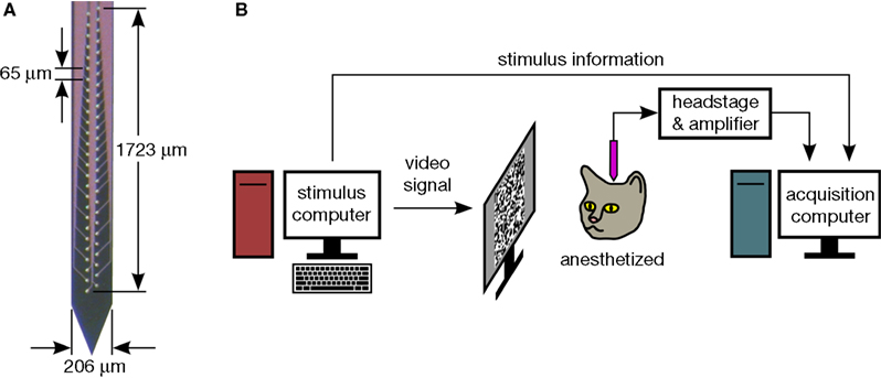
Figure 1. (A) One of several 54-channel silicon polytrode designs used. Recording sites are closely spaced, such that a spike will typically appear on several sites at the same time (see Figure 3
). (B) Experimental setup. Stimuli are presented to the animal while stimulus information and extracellular voltage waveforms are acquired and saved to disk.
The first of those tackled was visual stimulation. After an extensive search for existing software, we discovered the “Vision Egg” (Straw, 2008
), a Python library for generating stimuli. We chose the Vision Egg partly because of the language it was written in and written for: Python. We were thus introduced to Python via one of its many packages, and the experience was so positive that it encouraged us to standardize on Python for the spike sorting and spike train analysis projects to follow. For one of us (M. Spacek), the switch to Python has made programming a much more enjoyable and productive experience, and has resulted in greatly improved programming skills.
The benefits of Python have been extolled at length elsewhere (Hetland, 2005
; Langtangen, 2008
; Lutz, 2006
). Briefly, Python is a powerful, dynamically typed, interpreted language that “fits your brain”, with syntax akin to “executable pseudocode”. Python’s clear, simple syntax is perhaps its biggest selling point. Some of its clarity stems from a philosophy to provide “one – and preferably only one – obvious way” to do a given task (Peters, 2004
), making features easy to remember. Its clarity is also due to a strong adherence to object-oriented programming principles [Chapter 7 of Hetland (2005)
is an excellent introduction]. In Python, nearly everything is an object, even numbers and functions. This means that everything has attributes and methods (methods are functions that are bound to and act on objects), and can thus be treated in a similar way. An object is an instance of a class. A class can inherit attributes and methods from other classes hierarchically, allowing for substantial code reuse, and therefore less code to maintain. Python code is succinct compared to most other languages: a lot can be accomplished in only a few lines. Finally, Python is free and open source, and encourages open source software development. This is partly due to its interpreted nature: the source code and executable are typically one and the same.
Python has a stable and feature-rich numeric library called NumPy
1
which provides an N-dimensional array object. NumPy arrays can be subjected to vectorized operations, most of which call static C functions, allowing them to run almost as fast as pure C code. Yet, these operations remain accessible from within succinct Python code. NumPy turns Python into an effective replacement for MatLab (The MathWorks, Natick, MA, USA), and is used extensively by dimstim, spyke, and neuropy.
While all three projects presented here were written in Python, their use and implementation are very different. Dimstim is script based and is run from the system’s command line. Spyke has a graphical user interface (GUI) and looks like a native application, while neuropy is typically accessed from the Python command line as a library. Here, we explore some of the features and benefits of Python and its many add-on packages for the electrophysiologist, by introducing our own three packages as detailed working examples.
In our experiments, we needed a way to display and control a wide variety of stimuli with many different parameters, often shuffled with respect to each other in various ways. Since spike times are acquired at sub-millisecond temporal resolution, and since precise spike timing may play a role in neural coding (Mainen and Sejnowski, 1995
; VanRullen and Thorpe, 2002
), we also wanted high temporal precision in the stimulus. Our prior stimulus software was written in Fortran and ran under DOS with a 32-bit extender. It was written for the 8514/A graphics standard which has now lapsed. The last graphics cards to support it were limited in the size and speed of movie frames they could draw to screen. Moreover, these cards were limited to a screen refresh rate of 100 Hz at our desired resolution. We found significant artefactual phase-locking of responses in visual cortex at this frequency (Blanche, 2005
), which has been a concern reported elsewhere (Williams et al., 2004
; Wollman and Palmer, 1995
). For these reasons, we needed a better solution.
Dimstim displays full-screen stimuli at a refresh rate of 200 Hz, providing precise control of the display at 5 ms intervals without frame drops. Stimuli include manually controlled, drifting, and flashed bars and gratings, sparse noise, and m-sequence noise (Golomb, 1967
) and natural scene movies. Stimulus parameters can be shuffled with or without replacement, independently or in covariation with each other. Parameters include spatial location and phase, orientation, speed, duration, size, mask, contrast, brightness, and spatial and temporal frequencies. Each stimulus session is fully specified by its own user-editable script. A copy of the script, and an index of the contents of the screen on each screen refresh, are sent to the acquisition computer, for simultaneous recording of stimulus and neuronal responses.
Dimstim relies heavily on the Vision Egg
2
library (Straw, 2008
) to generate stimuli. The Vision Egg uses the well-established OpenGL
3
graphics language, which thanks to the demands of video games, is now supported by all modern video cards on all major platforms. We currently use an Nvidia GeForce 7600 graphics card running under Windows XP. Stimuli are displayed on a 19quotidnquotidn Iiyama HM903DTB and a 22quotidnquotidn HM204DTA CRT monitor, two of only a handful of consumer monitors that are capable of 800 × 600 resolution at 200 Hz. Unfortunately, like most other CRTs, these particular models have now been discontinued, but used ones may still be available. Hopefully the timing of LCD monitors will improve such that they can replace CRTs for temporally precise stimulus control.
Multitasking operating systems (OSes) present a challenge for real-time control of the screen. Often, the OS will decide to delay an operation to maintain responsiveness in other areas. This can lead to frame drops, but can be mitigated by increasing the priority of the Python process. Setting the process and thread priorities to their maximum levels in the Vision Egg completely eliminated frame drops in Windows XP, but with the unfortunate loss of mouse and keyboard polling. In dimstim, this meant that the user had no way of interrupting the stimulus script, other than by resetting the computer. Moving to a computer with a dual core CPU alleviated this problem, as the maximum priority Python process was delegated to one core without interruption, while other OS tasks such as keyboard polling ran normally on the second core.
Dimstim communicates stimulus parameters on a frame-by-frame basis to the acquisition computer via a PCI digital output board (DT340, Data Translations, Marlboro, MA, USA), for simultaneous recording of stimulus timing alongside neuronal responses. Parameters are described by sending the row index of a large lookup table (“sweep table”) on every screen refresh. The sweep table contains all the combinations of the dynamic parameters, i.e. those stimulus parameters that can vary from one screen refresh to the next.
The digital output board is controlled by its driver’s C library. Because Python is written in C (other implementations also exist), it has a C application programming interface (API), and extensions to Python can be written in C. We wrote such an extension to interact with the board’s C library, but today this is no longer necessary. A new built-in Python module called “ctypes” now allows interaction with a C library on any platform directly from within Python code. This is much simpler, as it removes the need to both write and compile C extension code using Python’s somewhat tedious C API. If dimstim were rewritten today, ctypes would be the method of choice. Dimstim includes a demo (
olda_demo.py) of how to use ctypes to directly interact with Data Translations’ Open Layers data acquisition library. Libraries for cards from other vendors (such as National Instruments’ NI-DAQmx) can be similarly accessed.Frame timing was tested with a photodiode placed on the monitor. The photodiode signal, along with the raster signal from the video card and the digital outputs from the stimulus computer, were all recorded simultaneously. We discovered that the contents of the screen always lagged by one screen refresh, due to OpenGL’s buffer swapping behaviour (Straw, 2008
). This was corrected for by adding one frame time (5 ms) to the timestamp of the digitized raster signal in the acquisition system.
Gamma correction was used to ensure linear control of screen luminance. Several levels of uncorrected luminance were measured with a light meter (Minolta LS-100) and fit to a power law expression to determine the exponent corresponding to the gamma value of the screen (Blanche, 2005
; Straw, 2008
). Gamma correction can be set independently for each script, or globally across all scripts in dimstim’s config file.
Natural scene movies used by dimstim were filmed outdoors with an ordinary compact digital camera (Canon PowerShot SD200) with 320 × 240 resolution at 60 frames per second (fps). Unfortunately, this camera could record no more than 1 min of video at a time. To generate longer movies, multiple clips were filmed in succession, while keeping the camera as motionless as possible between the end of one clip and the start of the next. Concatenation of and conversion from multiple colour .avi files to a single uncompressed greyscale movie file was done using David McNab’s y4m
4
package. Processed movies were displayed in dimstim with the same visual angle subtended by the camera, at 67 fps (three 5 ms screen refreshes per movie frame).
Usage
Dimstim’s config file stores default values for a variety of generic parameters that apply to most stimuli. These parameters include spatial location, size, orientation offset, and temporal and spatial frequencies. For simplicity, all spatial parameters are specified in degrees of visual angle. The config file can be edited by hand, but the typical procedure when optimizing parameters for the current neural population is to run a manually controlled bar or grating stimulus. For user convenience, the stimulus is shown simultaneously on two displays driven by two video outputs from the graphics card: one for the animal, and one for the user. The parameters of the manual stimulus are controlled in real-time with the mouse and keyboard. Once the user is satisfied, the parameters are saved to the config file. These can later be retrieved by an experiment script for use as default values.
An example script for a drifting sinusoidal grating experiment is shown in Figure 2
. The script works in a bottom-up fashion. First, objects for storage of static and dynamic parameters are instantiated (“s” and “d” respectively, lines 5–6). To these are bound various different parameters as attributes (denoted by a “ . ”). In this example, most values are declared directly by the script, but two static parameters, grating orientation offset and gamma correction, are retrieved from their defaults in the config file, using the dimstim config parser object named “dc” (lines 15 and 23). Dynamic parameters, if assigned a list of multiple values, will iterate over those values over the course of the experiment. In this case, grating orientation, spatial frequency, and temporal frequency are all assigned multiple values (lines 28, 36, 38). The rest remain constant for the duration of the experiment. In order to describe their interdependence and shuffling, each multiple-value dynamic parameter must be declared as a “Variable” (lines 53–55). Variables with the same dimension value (“dim” keyword argument) covary with each other, and must therefore all have the same number of values and the same shuffle flag. Variables with different dimension values vary independently in a combinatorial fashion, with the lowest numbered dimension varying slowest, and the highest varying fastest. This is implemented by dynamically generating a string object containing Python code with the correct number of nested for loops (equalling the number of independent variables specified in the script), and then executing the contents of the string with Python’s
exec() function (see the dimstim.Core.SweepTable class). Next, the number of times to cycle through all combinations, and the frequency at which to insert a blank screen sweep (for determining baseline firing rates) are specified in their own objects (lines 57–58). Finally, all these objects are passed together to the Grating class (which like all other dimstim stimuli, inherits from the Experiment class) to instantiate a Grating experiment object, and the experiment is run (lines 62–65). With 12 orientations,
6 spatial frequencies, and 4 temporal frequencies, this experiment has 288 unique parameter combinations, presented in shuffled order. Each is presented four times for a total of 1152 stimulus sweeps, lasting 4 s each, for a total experiment time of about 77 min (not including blank sweeps).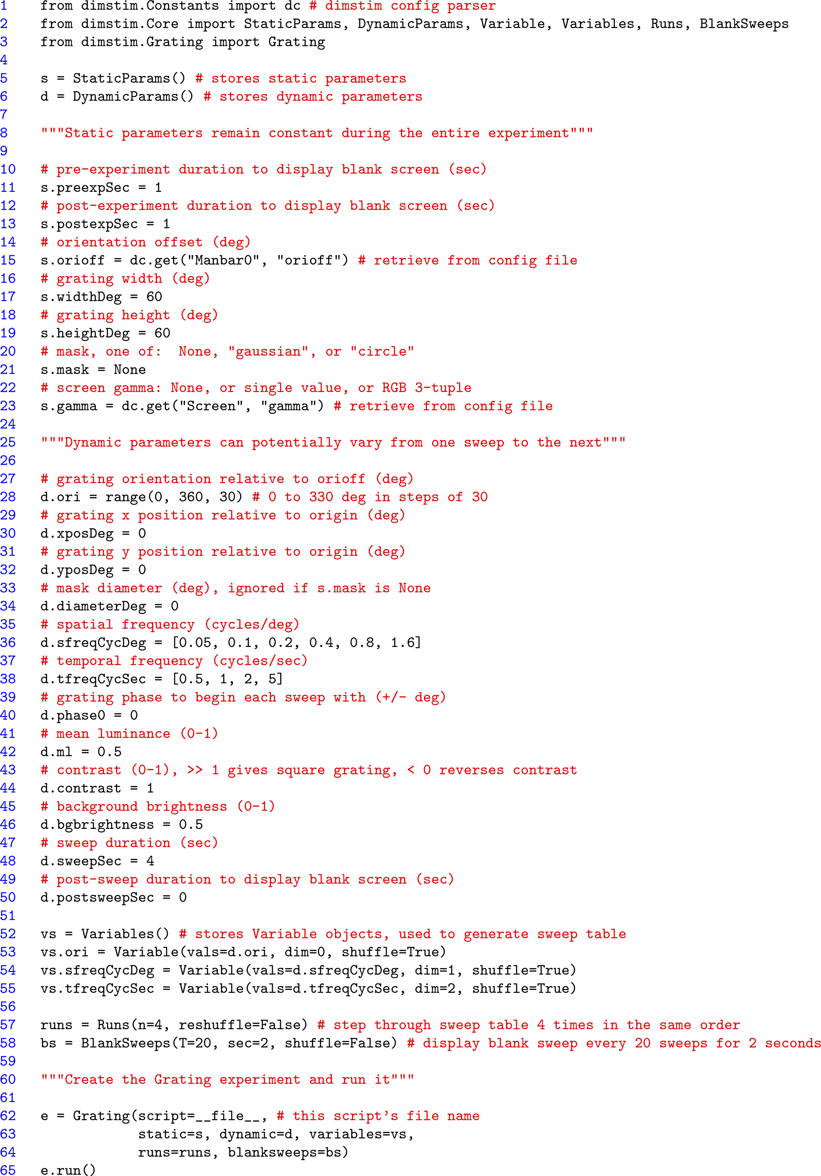
Figure 2. A dimstim script describing a drifting sinusoidal grating. Such scripts may be edited at will, and are the primary way the user interacts with dimstim. After some error checking, the script executes from the system’s command line, to which status messages are printed. Comments, denoted by # and """ in Python, are highlighted in red. Line numbers have been added for reference. See text for more details.
Before running, various checks are done to alert for any obvious errors in the user edited script. Then, a copy of the entire script is sent to the acquisition computer. This makes it possible to later reconstruct the sweep table for analysis, and even replay the entire experiment exactly, without the need for access to the original script on the stimulus computer. To ensure accurate timing, stimuli run only on the animal display, while the user display shows the system command line. In between experiments when no stimuli are running, a blank grey desktop is shown on the animal display. Scripts can be paused or cancelled using the keyboard.
Once neural waveform and stimulus data were saved to disk by our acquisition system (written in Delphi), we needed a way to retrieve the data for visualization and spike sorting. Our existing program for this, also written in Delphi, had some bugs and missing features. However, the Delphi environment required a license, the program would only run in Windows, and the code was more procedural than object-oriented. In particular, some of the code had blocks (if statements, for/while statements) that were nested many layers deep, making it difficult to follow. “Flat is better than nested” (Peters, 2004
) is another Python philosophy. Several short, shallow blocks of code are easier to understand and manage than one long deep block. We decided to start from scratch in Python.
Spyke has a cross-platform GUI with native widgets for data visualization and navigation, and spike sorting (Figure 3
). Spike waveforms are displayed in two ways: spatially according to the polytrode channel layout (spike window), and vertically in chart form (chart window). Local field potential (LFP) waveforms are also displayed vertically in chart form (LFP window). Polytrode channels are closely spaced (43–75 μm) over two or three columns (Figure 1
A). A single spike can generate a signal on multiple channels, hence the need to visualize waveforms according to their polytrode channel layout. Channels are colour-coded to make them easy to distinguish and align across windows. Spyke looks and behaves like a native GUI application, with menus, buttons, and resizable windows. Navigation is mouse and keyboard based. A horizontal slider and combo box at the top of the main spyke window control file position in time. Left and right arrow keys, and page up and page down keys step through the data with single timepoint or 1 ms resolution respectively. Clicking on any data window (spike, chart, or LFP) centres all three windows on that timepoint. Holding CTRL and scrolling the mouse wheel over a data window zooms it in or out in time. Holding CTRL and clicking on a channel enables or disables it. Hovering the mouse over a data window displays a tooltip with the timestamp, channel, and voltage currently under the mouse cursor.
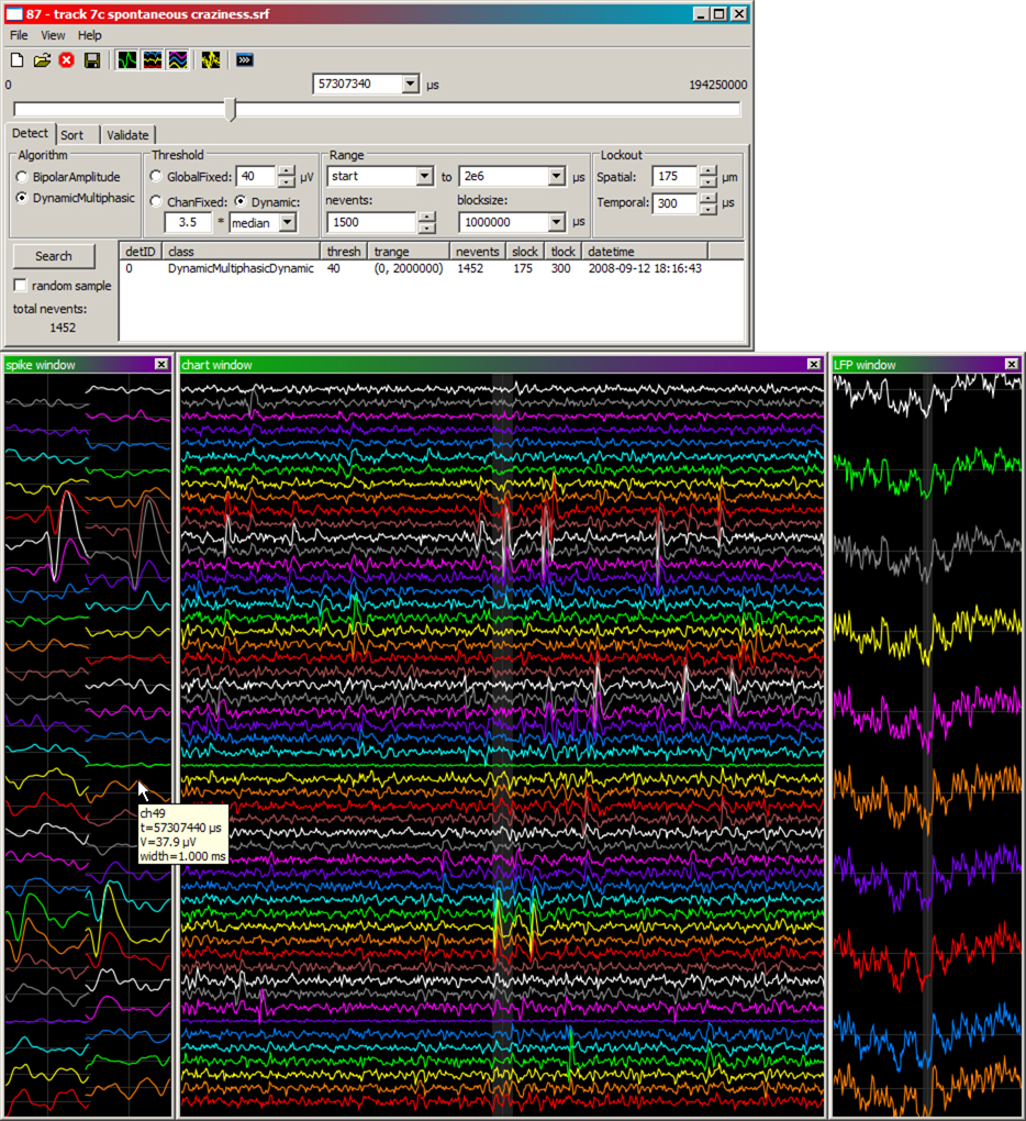
Figure 3. Main spyke window (top), with data windows (bottom) showing high-pass waveforms in polytrode layout (left ) and chart layout (middle). A third data window shows the low-pass LFP waveforms (right) concurrently recorded from a subset of channels (colour coded). All data are centred on the same timepoint. The shaded region in the middle of both the chart and LFP windows represents the time range spanned by the window to its left.
Spyke uses the wxPython
5
library for its GUI. This is a Python interface to the wxWidgets C++ GUI library which generates widgets on Windows, Linux, and OSX. Now well over a decade old (Rappin and Dunn, 2006
), wxPython is a stable library that has adapted to changing OSes. Widgets include everything from windows, menus, and buttons, to more complex list and tree controls. WxPython has a big advantage over other GUI libraries in its use of widgets that are native to the OS the program is running on, such that they look and behave identically to normally created widgets in that OS. WxGlade
6
was used to visually lay out the GUI. Itself a wxPython based GUI application, wxGlade takes the programmer’s visual layout and automatically generates the corresponding layout code in Python. This code can then be included in the programmer’s own code base, typically by defining a class that inherits from the automatically generated code. Although wxGlade is not necessary for writing a GUI with wxPython, we found it much faster and easier than writing all of the layout code by hand.
Unfortunately, some widgets are inherently different on different OSes. Writing and testing a wxPython GUI on only one OS will therefore not guarantee perfect functionality on another. To do so would require checking for the current OS, and implementing certain things differently depending on the OS. Spyke does not currently do this, and has so far only been thoroughly tested in Windows. A cross-platform GUI library faces many challenges. Although wxPython is one of the best (Rappin and Dunn, 2006
), it has bugs
7
– some of them longstanding – that had to be worked around in spyke.
Although the widgets are handled by wxPython, waveforms are plotted using matplotlib
8
. Matplotlib is a 2D plotting library for Python that generates publication quality figures. It has two interfaces: one that mimics the familiar plotting commands of MatLab, and another that is much more object-oriented. Spyke embeds matplotlib figures within wxPython windows. Scaling of plots is handled automatically by matplotlib, such that when the wxPython window is resized by dragging its corner or edge, the plotted traces inside resize accordingly. Another benefit of matplotlib is its antialiasing abilities, providing beautiful output with subpixel resolution. There is some performance penalty for using such a high level drawing library, but performance is fast enough on fairly ordinary hardware (Pentium M 1.6 GHz notebook), even when scrolling through 54 channels of data with thousands of data points on screen at a time. More importantly, matplotlib makes plotting very easy to do.
The data acquisition files are complex, with different types of data multiplexed throughout the file. On opening, the file must be parsed to determine the number and offset values of hundreds of thousands of records in the file. For multi GB files, this can take up to a few minutes. To deal with this, the parsing information is saved to disk for quicker future retrieval. This is done using Python’s
pickle module, which can take a snapshot of almost any Python object in memory, serialize it, and save it to disk as a “pickle”. A pickle can then later be restored (unpickled) to memory as a live Python object, even on a different platform. In this case, a custom written File object containing all of the parse information is saved to disk as a .parse file of only a few MB in size. Restoring from the .parse file is about an order of magnitude faster than reparsing the entire acquisition file.Segments of waveform data are loaded from the acquisition file, Nyquist interpolated, and sample-and-hold delay (SHD) corrected on the fly as needed (Blanche and Swindale, 2006
). Interpolation is performed to improve spike detection, and Nyquist interpolation is the optimum method of reconstructing a bandwidth-limited signal at arbitrary resolution. To do so, a set of sinc function kernels is generated (one kernel per interpolated data point, each kernel with a different phase offset) and convolved with the data. For SHD correction, a different set of kernels is generated for each channel. Correcting for each channel’s SHD requires appropriate modification of the phase offset of each kernel for that channel. For example, interpolating from 25 to 50 kHz with SHD correction requires two appropriately phase corrected kernels per channel. Each kernel is separately convolved with the data (using
numpy.convolve()), and the resulting data points are interleaved to return the final interpolated waveform.Spike Sorting
Spike sorting is done by template matching (Blanche, 2005
). Event detection is the first step in generating the required multichannel spike templates. Two event detection methods are currently implemented. The “bipolar amplitude” method looks for simple threshold crossings of either polarity. The “dynamic multiphasic” method searches for two consecutive threshold crossings of opposite polarity within a defined period of time. The second crossing’s threshold is dynamically set according to the amplitude of the first phase of the spike. For both methods, primary thresholds are calculated separately for each channel, based on the standard deviation or median noise level of either the entire recording or of a narrow sliding window thereof. Spatiotemporal detection lockouts prevent double triggering off of the same spike, while minimizing the chance of missed spikes.
Some algorithms, such as these event detection methods, cannot be easily vectorized and require a custom loop. Due to its dynamic typing and interpreted nature, long loops are slow to execute in Python. For the majority of software development, this is not an issue. Developer time is usually much more valuable than CPU time (Hetland, 2005
), but numerically intensive software is the exception. Writing fast Python extensions in C has always been possible, but the C interface code required by Python’s API is tedious to write, and writing in C eliminates the convenience of working in Python syntax. To get around this, the Cython
9
package (a fork of the Pyrex package) specifies a sublanguage almost identical to Python, with some extra keywords to declare loop variables as static C types. After issuing the standard
python setup.py build command, such code is automatically translated into an intermediary C file including all of the tedious interface code. This is subsequently compiled into object code and is accessible as a standard C extension module from within Python, just as a handwritten C extension would be. This yields the computational speed of C loops when needed, with the developmental speed, convenience and familiarity of Python syntax to implement them. Cython was used to write the custom loop that iterates over timepoints and channels for each of the event detection methods. For 25 kHz sampled waveform data on 54 channels, this amounts to 1.35 million iterations per second of data. On an average single-core notebook computer (Pentium M 1.6 GHz), this loop runs at about 5× real time.The data is partitioned into blocks (typically 1 s long), and each is searched independently, allowing multiple core CPUs to be exploited. Search speed scales roughly proportionally with the number of cores available. Due to the “global interpreter lock” (GIL) in the C implementation of Python, multiple processes must typically be used instead of multiple threads to take advantage of multiple cores. Unfortunately, a process can require significantly more memory and more time to create than a thread. There are ways around the GIL, but the best solution for spyke is not yet clear.
Search options are controlled in the “detect” tab in spyke’s main window (Figure 3
). Searches can be limited to specific time ranges in the file, in the number of events detected, and whether to search linearly or randomly. Random sampling is important to build up a temporally unbiased collection of detected events with which to build templates. Searching for the next or previous spike relative to the current timestamp can be done quickly using the keyboard. Searches are restricted to enabled channels, allowing for a targeted increase in the number of events belonging to a spatially localized template. This is useful for building up templates of neurons that rarely fire.
When a search completes, the sort window (Figure 4
A) opens and is populated with any newly detected events. The user then visually sorts the detected events (typically only a fraction of all spikes in the recording) into templates corresponding to isolated neurons. This is accomplished by plotting spikes over top of each other. Any number of event or template mean waveforms can be overplotted with each other. Although the mouse may be used, keyboard commands are more efficient for toggling the display of events and templates, and moving events and keyboard focus around between the sorted template tree (left column) and unsorted event list (right column). The event list has sortable columns for event ID, maximum channel, timestamp, and match error. All the events in the list can be matched against the currently selected template, and those match errors populate the error column. Sorting the event list by maximum channel or match error makes manual template generation much easier, because it clusters similar events close to each other in the unsorted event list.
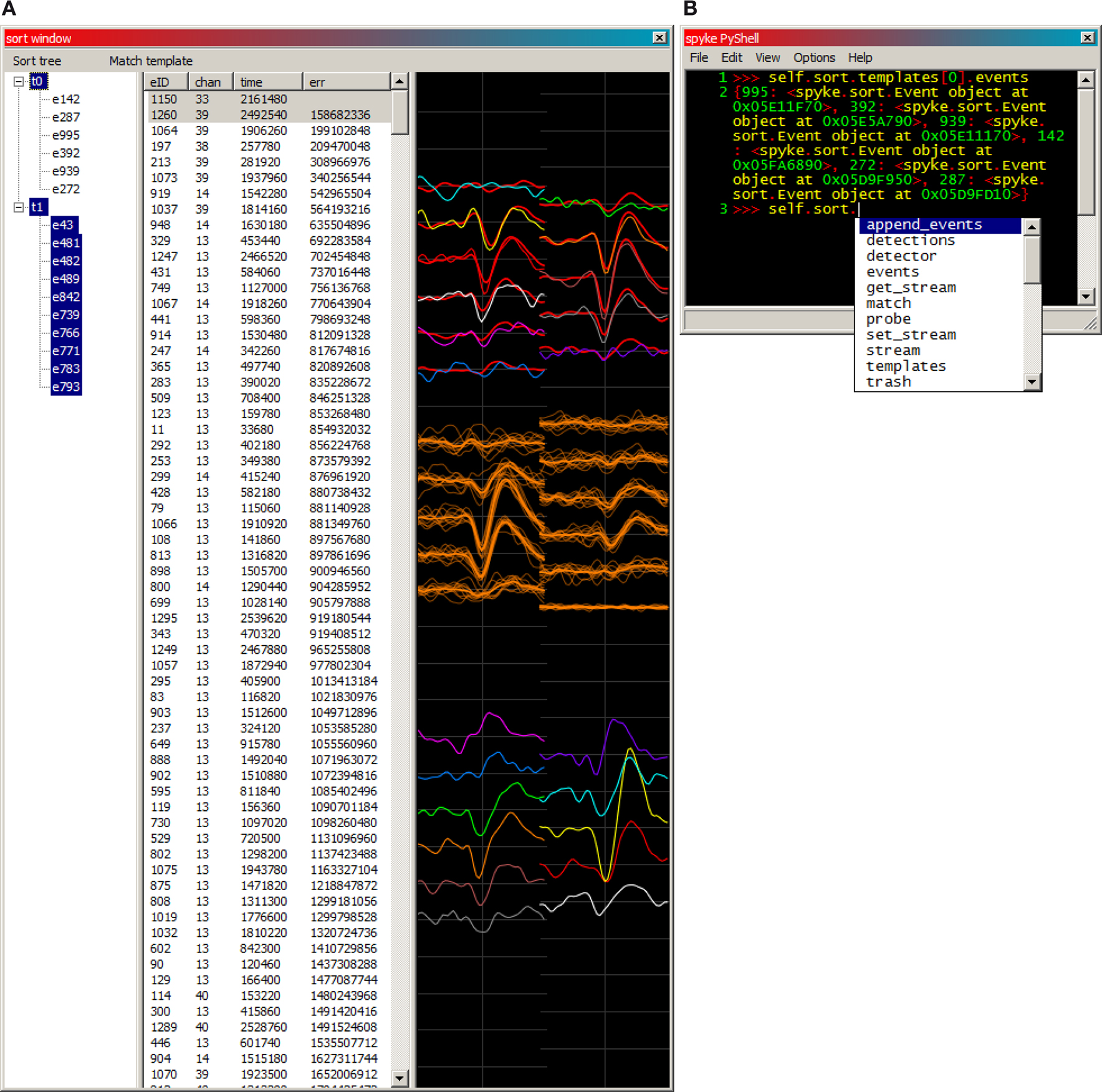
Figure 4. (A) An example of spyke’s sort window. Templates and their member spikes are represented in the tree (left), and unsorted detected events in the list (middle). Selecting a template or event in either the tree or the list plots its waveform (right). The tree currently has keyboard focus, making its selections more distinctly coloured than those of the list. Unsorted events have colour coded channels, while each template (and its member spikes) has a single identifying colour. Here, template 0 (red), a putative neuron near the top of the polytrode, has 6 member spikes, and its mean waveform is being overplotted with an unsorted event (#1260, multicoloured), which fits quite well. Template 1 (orange) and all of its member spikes are plotted near the middle of the polytrode. Also plotted further down is another unsorted event (#1150, multicoloured), which obviously does not fit either template. The error values listed are from a match against template 0. (B) The integrated PyShell window exposes all of spyke’s objects and functionality at the Python command line. Template 0’s dictionary (a mapping from names to values) of its 6 member events is referenced and returned on lines 1–2. The “Sort” object’s attributes and methods are displayed in a popup on line 3.
Once templates have been generated, a full event detection is run across the whole recording, and the templates are matched against each detected event. Or, each template can be slid across the recording and matched against every timepoint in the recording (Blanche et al., 2005
). Either way, matching to target and non-target spikes or noise generally yields a non-overlapping bimodal error distribution. For each template, a threshold is manually set at the trough between the two peaks in the distribution, and events whose match errors fall below this threshold are classified as spikes of that template.
At any point in the sorting process, the entire “Sort” session object, which among other information includes detected events, generated templates, and sorted spikes, can be saved to disk as a .sort file, again using Python’s
pickle module. Sort sessions can then be restored from disk and sorting can resume in spyke, or their sorted spike times can be used for spike train analysis (see neuropy section). Waveform data for detected events and sorted spikes is saved within the .sort file. This increases the file size, but allows for review of detected and sorted spikes without the need to access the original multi GB continuous data acquisition file.Integrated into spyke is Patrick O’Brien’s PyShell (Figure 4
B), an enhanced Python command line that is part of the wxPython package. This permits live command line inspection and modification of all objects comprising spyke. This was, and continues to be, a very useful tool for testing existing features and for developing new ones. Neuropy (or almost any other Python package) can be imported and used directly from this command line. For example, spike sorting validation is not yet implemented in spyke’s GUI, but all of neuropy’s functionality including autocorrelograms (to check refractory periods) can be accessed by typing
import neuropy in spyke’s PyShell.After spike sorting, we needed a way to analyse spike trains and their relation to stimuli. Our initial decision was to use MatLab for spike train analysis, and we soon developed a collection of MatLab scripts for the job, with one function per .m file. For example, one .m file would load each neuron’s data from disk and return all of them in a cell array of structures. This was highly procedural instead of object-oriented. Furthermore, the code became difficult to manage as each additional function required an additional .m file. We were also faced with out of memory errors, limited GUI capabilities, and a high licensing cost.
Although MatLab’s toolboxes are a major benefit, SciPy
10
(Jones et al., 2001
), an extensive Python library of scientific routines, provides most of the equivalent functionality. Much of SciPy is a wrapper for decades-old, highly tested and optimized Fortran code. Another package, mlabwrap
11
, allows a licensed MatLab user to access all of MatLab’s functionality, including all of its toolboxes, directly from within Python. Although in the end we did not need to use mlabwrap, its existence erased any remaining hesitations about switching to Python for analysis.
A data-centric object hierarchy (Figure 5
A) quickly emerged as a natural way to organize neuropy. Each object in the hierarchy has an attribute that references its parent object, as well as all of its child objects. Specifically, “Data” is an abstract object from which all “Animals” are accessible. Each Animal has polytrode “Tracks”, each Track has “Recordings”, and each Recording has both “Sorts” (spike sorting sessions) and “Experiments” (which describe stimuli). Finally, each Sort contains a number of “Neurons”, one of whose attributes is a NumPy array of spike times.
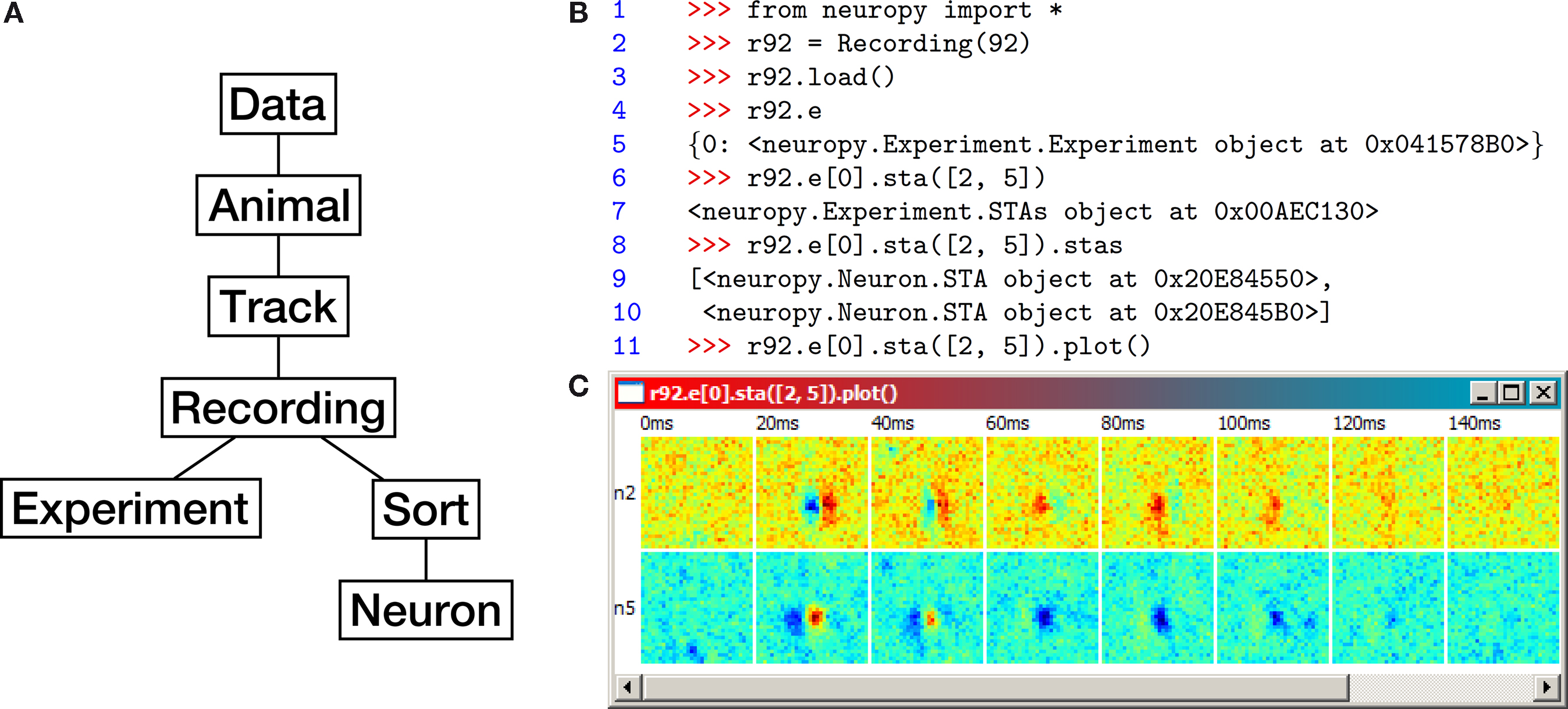
Figure 5. (A) Neuropy’s object hierarchy. (B) Example code using neuropy to plot the spike-triggered average (STA) of two neurons in response to an
m-sequence noise movie (see text for details). (C) The resulting plot window. Each row corresponds to a neuron, and each column corresponds to the
STA within a fixed time range following the m-sequence white noise stimulus. ON responses are red, OFF responses are blue.
Neuropy relies on a hierarchy of data folders on the disk with a fairly rigid naming scheme, such that animal, track, recording, experiment, and sort IDs can be extracted from file and folder names. This forces the user to keep sorted data organized. All objects have a unique ID under the scope of their parent, but not necessarily under the scope of their grandparent. All data can be loaded in at once by creating an instance of the Data class and then calling its .load() method. However, most often only a subset of data is needed, such as only the data from a given animal, track, or recording. For example, an object representing recording 92 from the default track of the default animal can be instantiated by typing
Recording(92) at the command line. This recording’s data can then be loaded from disk into the object by calling its .load() method. Default animal and track IDs can be modified from the command line. A recording loads the neurons from its default sort, which can also be modified.Some analyses are written as simple methods of one of the data objects, but most have their own separate class which is instantiated by a data object’s method call. Many analyses generate plots, some of them interactive (such as the population spike raster plot), again using matplotlib and wxPython. Currently implemented analyses include interspike interval histograms, instantaneous firing rates and their distributions, cross-correlograms and autocorrelograms, and spike-triggered averages (STAs) (Dayan and Abbott, 2001
). More specialized analyses include binary codes of population spike trains, their correlation coefficient distributions, maximum entropy Ising modelling of such codes (using
scipy.maxent), and several other related analyses (Schneidman et al., 2006
; Shlens et al., 2006
; Spacek et al., 2007
). Because of the data-centric organization, new analyses are easy to add.Neuropy is used interactively as a library from the Python command prompt, usually in an enhanced shell such as PyShell (Figure 4
B) or the more widely used IPython
12
. An example of neuropy use is shown in Figure 5
B, which calculates and plots the STA of neurons 2 and 5 of the default animal and track. The STA estimates a neuron’s spatiotemporal receptive field by averaging the stimulus (in this case, an m-sequence noise movie) at fixed time intervals preceding each spike. Recording 92 was recorded during m-sequence noise movie playback, and is used in this example. Line 1 imports all of neuropy’s functionality into the local namespace. Next, an object representing recording 92 is instantiated and bound to the name
r92 for convenience, and its data is loaded from disk (lines 2–3). Its dictionary of available experiments is requested and printed out (lines 4–5); only one experiment is available, with ID 0. STAs are calculated with respect to this experiment by calling its .sta() method and passing the IDs of the desired neurons (line 6). The calculated STAs are returned in an “STAs” object, which upon further inspection contains two “STA” objects, one per requested neuron (lines 7–10). Finally, the STAs object’s .plot() method is called with default options, displaying the result for both neurons (Figure 5
C).Python’s object orientation has benefits even at the command line. It allows the user to quickly discover what methods and attributes are available for any given object, eliminating the need to recall them from memory (Figure 4
B). Instead of immediately returning the raw result or plotting it, most analyses in neuropy return an analysis object, which usually has .calc() and .plot() methods. The .calc() method is run automatically on instantiation, and the results are stored as attributes of the analysis object. Settings used to do the calculation are also stored as attributes. These can be modified, and .calc() can be called again to update the result attributes. Once satisfied with the calculation, the user can call the .plot() method. This can be done several times to generate different plots with different plot settings. Each time a new plot is generated, it does so from the existing results, saving on unnecessary recalculation time.
We have described Python packages for three tasks pertinent to systems neuroscience: visual stimulus generation, waveform visualization and spike sorting, and spike train analysis. Python allowed us to meet these software challenges with a level of performance not normally associated with a dynamically typed interpreted language. Performance challenges included time-critical display and communication of visual stimuli, parsing and streaming of multiplexed data from GB sized files, on the fly Nyquist interpolation and SHD correction, fast execution of non-vectorizable algorithms, and parallelization. Other challenges, whose solutions were simpler than in a statically compiled language, included a cross-platform native GUI, the storage and retrieval of relatively complex data structures to and from file (.parse and .sort files), and a command line environment for interactive data analysis.
Dimstim is the oldest of the three packages, and the most stable. Spyke is the most recent and remains under heavy development, while new analyses are added to neuropy as needed. As with most other Python packages, all three can be used alone or from within another Python module. All three depend on each other to a limited extent. Neuropy relies on the stimulus description and timing signals generated by dimstim, and on the spike sorting results from spyke. Spyke can use parts of neuropy for spike sorting validation. These three packages depend on many other open source packages, which themselves rely on yet other packages (e.g. the Vision Egg currently depends on PyOpenGL and PyGame). Modularity and code reuse is thus maximized across the community.
Because it greatly encourages object-oriented programming, Python code is easier to organize and reuse than MatLab code. This is important for scientific code which tends to continually evolve as new avenues are explored. Often, scientific code is quickly written and bug-tested, used once or twice, and then forgotten about, with little chance of re-use outside of copying and pasting. Python has reduced this tendency for us. Its object orientation and excellent error handling have also helped to reduce bugs.
Finally, Python was chosen for these projects for its clear, succinct syntax. Dimstim, spyke, and neuropy have roughly 3000, 5000, and 4000 lines of code respectively (excluding comments and blank lines). Fewer lines make code maintenance easier, not just because there is less code to maintain, but also because each line is closer to all other lines, making it easier to navigate. Concise syntax also makes collaboration easier.
We encourage others in neuroscience to consider Python for their programming needs, and hope that our three examples (available at
http://swindale.ecc.ubc.ca/code
) may be of use to others, whether directly or otherwise. Rallying around a common open-source language may help foster efforts to increase sharing of data and code, efforts deemed necessary (Teeters et al., 2008
) to push forward progress in systems neuroscience.The authors declare that the research was conducted in the absence of any commercial or financial relationships that could be construed as a potential conflict of interest.
Keith Godfrey wrote dimstim’s C extension to interface with the Data Translations board. Reza Lotun contributed code to early versions of spyke. Funding came from grants from the Canadian Institutes of Health Research, and the Natural Sciences and Engineering Research Council of Canada.
- ^
http://numpy.org - ^
http://visionegg.org - ^
http://opengl.org - ^
http://freenet.org.nz/y4m - ^
http://wxpython.org - ^
http://wxglade.sf.net - ^
See bugs #626 and #2307 at
http://trac.wxwidgets.org - ^
http://matplotlib.sf.net - ^
http://cython.org - ^
http://scipy.org - ^
http://mlabwrap.sf.net - ^
http://ipython.scipy.org
Jones, E., Oliphant, T., Peterson, P., et al. (2001). SciPy: open source scientific tools for Python. http://scipy.org.
Peters, T. (2004). The Zen of Python. http://www.python.org/dev/peps/
pep-0020.
Spacek, M. A., Blanche, T. J., Seamans, J. K., and Swindale, N. V. (2007). Accounting for network states in cortex: are (local) pairwise correlations sufficient? Soc. Neurosci. Abstr. 33, 790.1. http://swindale.ecc.ubc.ca/Publications.