Regression with Ordered Predictors via Ordinal Smoothing Splines
 Nathaniel E. Helwig
- 1Department of Psychology, University of Minnesota, Minneapolis, MN, United States
- 2School of Statistics, University of Minnesota, Minneapolis, MN, United States
Many applied studies collect one or more ordered categorical predictors, which do not fit neatly within classic regression frameworks. In most cases, ordinal predictors are treated as either nominal (unordered) variables or metric (continuous) variables in regression models, which is theoretically and/or computationally undesirable. In this paper, we discuss the benefit of taking a smoothing spline approach to the modeling of ordinal predictors. The purpose of this paper is to provide theoretical insight into the ordinal smoothing spline, as well as examples revealing the potential of the ordinal smoothing spline for various types of applied research. Specifically, we (i) derive the analytical form of the ordinal smoothing spline reproducing kernel, (ii) propose an ordinal smoothing spline isotonic regression estimator, (iii) prove an asymptotic equivalence between the ordinal and linear smoothing spline reproducing kernel functions, (iv) develop large sample approximations for the ordinal smoothing spline, and (v) demonstrate the use of ordinal smoothing splines for isotonic regression and semiparametric regression with multiple predictors. Our results reveal that the ordinal smoothing spline offers a flexible approach for incorporating ordered predictors in regression models, and has the benefit of being invariant to any monotonic transformation of the predictor scores.
1. Introduction
1.1. Motivation
The General Linear Model (GLM) (see [1]) is one of the most widely applied statistical methods, with applications common in psychology [2], education [3], medicine [4], business [5], and several other disciplines. The GLM's popularity in applied research is likely due to a combination of the model's interpretability and flexibility, as well as easy availability through R [6] and commercial statistical softwares (e.g., SAS, SPSS, etc.). The GLM and its generalized extension (GzLM; see [7]) are well-equipped for modeling relationships between variables of mixed types, i.e., unordered categorical and continuous variables can be simultaneously included as predictors in a regression model. However, many studies collect one (or more) ordered categorical variables, which do not fit neatly within the GLM framework.
For example, in finance it is typical to rate the risk of investments on an ordinal scale (very low risk, low risk, …, high risk, very high risk), and a typical goal is to model expected returns given an investment's risk. In medical studies, severity of symptoms (very low, low, …, high, very high) and adherence to treatment (never, rarely, …, almost always, always) are often measured on ordinal scales, and a typical goal is to study patient outcomes in response to different treatments after controlling for symptom severity and treatment adherence. Psychological attributes such as personality traits and intelligence are typically measured on an ordinal scale, e.g., using questionnaires consisting of Likert scale items (strongly disagree, disagree, …, agree, strongly agree), and many psychological studies hope to understand how individual and group differences in psychological traits relate to differences in observed behavioral outcomes.
The examples mentioned in the previous paragraph represent just a glimpse of the many ways in which ordinal variables are relevant to our day-to-day financial, physical, and mental health. When it comes to modeling ordinal outcome (response) variables, there are a multitude of potential methods discussed in the literature (see [8-12]). However, when it comes to including ordinal variables as predictors in a GLM (or GzLM), the choices are slim. In nearly all cases, ordinal predictors are treated as either nominal (unordered) or continuous variables in regression models, which can lead to convoluted and possibly misleading results.
Suppose X is an ordered categorical variable with K categories (levels) 1 < ⋯ < K, and suppose we want to include X as a predictor in a regression model. The naive method would be to include K − 1 dummy variables in the model design matrix, and let the intercept absorb the K-th level's effect. We refer to this method as naive for two reasons: (i) this approach ignores the fact that the levels of X are ordered and, instead, parameterizes X as K − 1 unrelated variables, and (ii) this approach makes it cumbersome (and possibly numerically unstable) to examine interaction effects involving ordinal predictors, which could be of interest in a variety of studies. Although the dummy coding approach will suffice for certain applications, this method is far from ideal. Furthermore, if the number of levels K is large, the dummy coding approach could be infeasible.
Another possibility for including an ordinal predictor X in a regression model is to simply treat X as a continuous variable. In some cases, researchers make an effort to code the levels of an ordinal predictor X such that the relationship between X and Y is approximately linear. This approach is parsimonious because the ordinal predictor with K categories (requiring K − 1 coefficients) will be a reduced to a continuous predictor with a linear effect (requiring 1 coefficient). However, this approach is problematic for several reasons (i) the slope coefficient in such a model has no meaning, (ii) different researchers could concoct different coding schemes for the same data, which would hinder research comparability and reproducibility, and (iii) the ordinal nature of the predictor X is ignored, which is undesirable.
Penalized regression provides a promising framework for including ordinal predictors in regression models [13], given that an appropriate penalty can simultaneously induce order information on the solution and stabilize the estimation. Gertheiss and Tutz [13] discuss how a binary design matrix in combination with a squared difference penalty can be used to fit regression models with ordinal predictors. This approach is implemented in the R package ordPens [14], which fits models containing additive effects of ordinal and metric (continuous) predictors. Adding a penalty to impose order and stabilize the solution is a promising approach, but this method still parameterizes X as K − 1 unrelated variables in the model design matrix. As a result, this approach (and the ordPens R package) offer no method for examining interaction effects between multiple ordinal predictors or interaction effects between ordinal and metric predictors.
1.2. Purpose
In this paper, we discuss the benefits of taking a smoothing spline approach [15, 16] to the modeling of ordinal predictors. This approach has been briefly mentioned as a possibility [15, p. 34], but a thorough treatment of the ordinal smoothing spline is lacking from the literature. Expanding the work of Gertheiss and Tutz [13] and Gu [15], we (Section 3.1) derive the analytical form of the reproducing kernel function corresponding to the ordinal smoothing spline, which makes it possible to efficiently compute ordinal smoothing splines. Our results reveal that the reproducing kernel function only depends on rank information, so the ordinal smoothing spline estimator is invariant to any monotonic transformation of the predictor scores. We also (Section 3.2) propose an ordinal smoothing spline isotonic regression estimator via factoring the reproducing kernel function into monotonic (step) functions. Furthermore, we (Section 3.3) prove a correspondence between the ordinal and linear smoothing spline for large values of K, and (Section 3.4) develop computationally scalable approximations for fitting ordinal smoothing splines with large values of K. Finally, we demonstrate the potential of the ordinal smoothing spline for applied research via a simulation study and two real data examples. Our simulation study (Section 4) reveals that the ordinal smoothing spline can outperform the linear smoothing spline and classic isotonic regression algorithms when analyzing monotonic functions with various degrees of smoothness. Our real data results (Section 5) demonstrate that the ordinal smoothing spline—in combination with the powerful smoothing spline ANOVA framework [15]—provides an appealing approach for including ordinal predictors in regression models.
2. Smoothing Spline Background
2.1. Reproducing Kernels
Let denote a Hilbert space of functions on domain , and let 〈·, ·〉 denote the inner-product of . According to the Riesz representation theorem [17, 18], if L is a continuous linear functional in a Hilbert space , then there exists a unique function such that Lη = 〈ζL, η〉 for all . The function ζL is referred to as the representer of the functional L. The evaluation functional [x]η = η(x) evaluates a function at an input . If the evaluation functional [x]η = η(x) is continuous in for all , then the space is referred to as a reproducing kernel Hilbert space (RKHS) (see [15, 16]). If is a RKHS with inner-product 〈·, ·〉, then there exists a unique function that is the representer of the evaluation functional [x](·), such that [x]η = 〈ρx, η〉 = η(x) for all and all . The symmetric and non-negative definite function
is called the reproducing kernel of because it satisfies the reproducing property 〈ρ(x, y), η(y)〉 = η(x) for all and all , see Aronszajn [19]. If with , then
where and are the reproducing kernels of and , respectively, such that
with 〈·, ·〉 = 〈·, ·〉0 + 〈·, ·〉1, , , and .
2.2. Smoothing Spline Definition
Assume a nonparametric regression model (see [15, 16, 20-23])
for i = 1, …, n, where yi ∈ ℝ is the real-valued response for the i-th observation, is the predictor for the i-th observation where is the predictor domain, is an unknown smooth function where is a RKHS with inner-product 〈·, ·〉, and is a Gaussian error term. A smoothing spline is the function ηλ that minimizes the penalized least squares functional
where J(·) is a quadratic penalty functional such that larger values correspond to less smoothness, and λ ≥ 0 is a smoothing parameter that balances the trade-off between fitting and smoothing the data. Let denote a tensor sum decomposition of , where is the null space of J and is the contrast space. Similarly, let 〈·, ·〉 = 〈·, ·〉0+〈·, ·〉1 denote the corresponding decomposition of the inner-product of . Note that, by definition, the quadratic penalty functional J is the inner-product of the contrast space , i.e., J(η) = 〈η, η〉1. Given λ, the Kimeldorf-Wahba representer theorem [24] states that the ηλ minimizing Equation (5) has the form
where the functions span the penalty's null space , the function ρ1 is the reproducing kernel of the contrast space , and d = {dv} and c = {ci} are the unknown coefficient vectors (see [15, 16, 25]). The reproducing property implies that the quadratic penalty functional J(ηλ) = 〈ηλ, ηλ〉1 has the form
which can be easily evaluated given ρ1, c, and x.
2.3. Types of Splines
The type of spline will depend on the forms of the RKHS and the inner-product 〈·, ·〉, which will depend on the predictor domain . The essential components for the formation of a smoothing spline include: (i) form a tensor sum decomposition of the RKHS , (ii) partition the inner-product of the RKHS 〈·, ·〉 = 〈·, ·〉0 + 〈·, ·〉1 such that 〈·, ·〉k defines an inner-product in for k ∈ {0, 1}, (iii) define the smoothing spline penalty as J(η) = 〈η, η〉1, and (iv) derive the reproducing kernels of and . Table 1 provides the information needed to form three common smoothing splines (nominal, polynomial, and thin-plate), as well as the ordinal smoothing spline. See Gu [15] and Helwig and Ma [26] for more information about nominal and polynomial smoothing splines, and see Gu [15], Helwig and Ma [26], Duchon [27], Meinguet [28], and Wood [29] for more information about thin-plate splines. More information about the ordinal smoothing spline will be provided in Section 3.
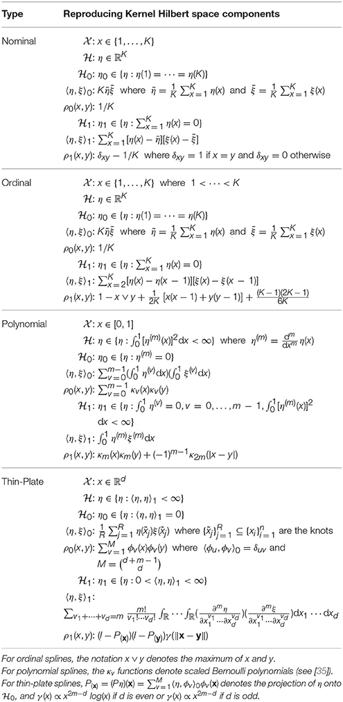
Table 1. Ingredients for forming different types of smoothing splines.
2.4. Tensor Product Smoothers
Suppose we have a model with predictor vector where . If the predictors are all continuous with similar scale, a thin-plate spline can be used. However, if the predictors differ in type and/or scale (e.g., some nominal and some continuous), another approach is needed. Let and denote two realizations of X and let
denote the reproducing kernel function corresponding to , which denotes a RKHS of functions on for j = 1, …, d. The symmetric and non-negative definite function
defines the unique tensor product reproducing kernel function corresponding to the tensor product RKHS
where with denoting the tensor product null space and with denoting the tensor product contrast space.
A tensor product smoothing spline solves the penalized least squares problem in Equation (5) in a tensor product RKHS . In this case, the contrast space can be decomposed such as where the are orthogonal subspaces with inner-products . The different may have different modules, so it is helpful to reweight the relative influence of each . Specifically, when solving the penalized least squares functional, we can define
where is the reproducing kernel of and θk > 0 are additional (non-negative) smoothing parameters that control the influence of each [see 15, 25, 26]. We can decompose any such as
where and for k = 1, …, s. Note that the different functions correspond to different nonparametric main and interaction effects between predictors, so different statistical models can be fit by removing different subspaces (and corresponding ) from the model.
2.5. Smoothing Spline Computation
Applying the Kimeldorf-Wahba representer theorem, we can approximate Equation (5) as
where is the response vector, K = {ϕv(xi)}n×m is the null space basis function matrix, denotes the contrast space basis function matrix with denoting the selected knots, and denotes the penalty matrix. The full solution uses all unique xi as knots, but using a subset of R ≪ n knots has been shown to perform well in practice, as long as enough knots are included to reasonably span [26, 30-32]. Given λ, the optimal coefficients are
where (·)† denotes the Moore-Pensore pseudoinverse [33, 34]. The fitted values can be written as
where
is the smoothing matrix, which depends on λ and any θk parameters embedded in ρ1. The smoothing parameters can be obtained by minimizing the Generalized Cross-Validation (GCV) criterion [35]
where tr(Sλ) is often considered the effective degrees of freedom of a smoothing spline.
2.6. Bayesian Interpretation
The smoothing spline solution in Equation (15) can be interpreted as a Bayesian estimate of a Gaussian process [36-40]. Suppose that where for k ∈ {0, 1}. Furthermore, assume that (i) where and , (ii) where and , and (iii) η0 and η1 are independent of one another and of the error term ϵ. Applying Bayes's Theorem, the posterior distribution of β = (d′, c′)′ is multivariate normal with mean and covariance
where is a block-diagonal matrix, , and . Letting τ2 → ∞ corresponds to a diffuse prior on the null space coefficients, and
makes the posterior mean equivalent to the smoothing spline coefficient estimates from Equation (14). The corresponding Bayesian covariance matrix estimator is
Using this Bayesian interpretation, one can form a 100(1 − α)% Bayesian “confidence interval” around the smoothing spline estimate
where ψ′ = (ϕ′, ρ′) and Zα/2 is a critical value from a standard normal distribution. These confidence intervals have a desirable across-the-function coverage property, such that the intervals are expected to contain about 100(1 − α)% of the function realizations, assuming that the GCV has been used to select the smoothing parameters [37, 38, 40].
3. Ordinal Smoothing Spline
3.1. Formulation
Real-valued functions on correspond to real-valued vectors of length K, where the function evaluation is equivalent to coordinate extraction, i.e., η(x) for x ∈ {1, …, K} can be viewed as extracting the x-th element of the vector . Thus, equipped with an inner product, the space of functions on is a RKHS, denoted by , which can be decomposed into the tensor summation of two orthogonal subspaces: . The null space consists of all constant functions (vectors of length K), and the contrast space consists of all functions (vectors of length K) that sum to zero across the K elements.
For ordinal predictors with 1 < ⋯ < K, we can use the penalty functional
which penalizes differences between adjacent values [13, 15]. Letting η = [η(1), …, η(K)]′, we can write the penalty functional as
where D = {dij}K−1 × K is a first order difference operator matrix with elements defined as
As an example, with K = 5 the matrix D has the form
The penalty functional in Equation (22) corresponds to the inner-product
where , , is the inner product of the null space, and is the inner product of the contrast space. Note that by definition. Furthermore, note that the ordinal smoothing spline estimates η within the same RKHS as the nominal smoothing spline (see Table 1), however the ordinal smoothing spline uses a different definition of the inner-product for the contrast space, which induces a different reproducing kernel.
Theorem 3.1. Given the ordinal smoothing spline inner-product in Equation (26), the null space has reproducing kernel ρ0(x, y) = 1/K, and the contrast space has reproducing kernel
for x, y ∈ {1, …, K} where 1{·} is an indicator function, x ∨ y = max(x, y), and .
See the Supplementary Material for a proof. Note that Theorem 3.1 provides the reproducing kernel needed to numerically evaluate the optimal ηλ from Equation (6) for the ordinal smoothing spline. Considering the model in Equation (4) with where 1 < ⋯ < K are elements of an ordered set, the penalized least squares problem has the form
where is the response vector, d is the unknown intercept, G = {gij}n×K is a selection matrix such that gij = 1 if xi = j for j ∈ {1, …, K} and gij = 0 otherwise, with and for i, j = 1, …, K, and are the unknown function coefficients. Given λ, the optimal coefficients and smoothing matrix can be obtained using the result in Equations (14) and (16) with K = 1n and J = GQ. When applying the Bayesian interpretation in Section 2.6, note that the pseudoinverse of Q has Toeplitz form for the internal rows and columns with deviations from Toeplitz form in cells (1,1) and (K, K). As an example, with K = 5 the pseudoinverse of Q is given by
where c ~ N(0, [σ2/(nλ)]Q†) is the assumed prior distribution for the contrast space coefficients.
3.2. Relation to Isotonic Regression
Using the reproducing kernel definition in the first line of Theorem 3.1, where the elements of the matrix M = {mij}K×K−1 have the form
As an example, with K = 5 the matrix M has the form
Note that the columns of M sum to zero, which implies that Q0Q = 0K×K, where is the reproducing kernel matrix for the null space. To visualize the ordinal smoothing spline reproducing kernel function, Figure 1 plots the columns of M and the columns of the corresponding reproducing kernel matrix Q for the situation with K = 5. Note that by definition (i) the K − 1 columns of M are (linearly independent) monotonic increasing functions of x ∈ {1, …, K} and (ii) the K columns of Q are linearly dependent given that Q has rank K − 1.
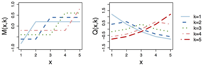
Figure 1. Visualization of the ordinal smoothing spline reproducing kernel function with K = 5 levels of X. Left plot shows the columns of the factorized kernel matrix M, whereas right plot shows the columns of reproducing kernel matrix Q = MM′.
The factorization of the reproducing kernel matrix Q = MM′ implies that the ordinal smoothing spline can be reformulated to form an isotonic regression estimator. Specifically, we could reparameterize the ordinal smoothing spline problem as
where and Q = MM′ by definition. Note that columns of M are monotonic increasing such that the k-th column contains two unique values with the “jump” occurring between rows k and k+1 for k ∈ {1, …, K−1}, see Figure 1. Thus, by constraining the elements of cm to be non-negative, we can constrain the ordinal smoothing spline to be a monotonic increasing function across the values 1 < ⋯ < K. Specifically, for a fixed λ we seek the solution to the problem
where is the coefficient vector, X = [1n, GM] is the design matrix, is a K×K identity matrix with cell (1,1) equal to zero, and A = (0K−1, IK−1) is the (K −1) × K constraint matrix.
Theorem 3.2. The coefficient vector β minimizing the inequality constrained optimization problem in Equation (32) has the form
where , is the unconstrained ordinal smoothing spline solution, and the A2 and B2 matrices depend on the active constraints.
See the Supplementary Material for the proof. Note that Theorem 3.2 reveals that the ordinal smoothing spline isotonic regression estimator is a linear transformation of the unconstrained estimator. Furthermore, Theorem 3.2 implies that where the smoothing matrix has the form . Thus, when the non-negativity constraints are active, can be used as an estimate of the effective degrees of freedom for smoothing parameter selection.
3.3. Reproducing Kernel as K → ∞
We now provide a theorem on the behavior of the ordinal smoothing spline reproducing kernel as the number of levels K of the ordered set approaches infinity.
Theorem 3.3. As K → ∞, we have where
is the ordinal smoothing spline reproducing kernel function for with x ∨ y = max(x, y) denoting the maximum of x and y, and
is the linear smoothing spline reproducing kernel function for with and ỹ = (y − 1)/(K − 1) by definition.
See the Supplementary Material for a proof. Note that Theorem 3.3 implies that ordinal and linear smoothing splines will perform similarly as the number of levels of the ordered set K increases. In Figure 2, we plot the reproducing kernel function for the (standardized) ordinal and linear smoothing spline (with K = 5), along with the Frobenius norm between the (standardized) ordinal and linear smoothing spline reproducing kernel matrices for different values of K. This figure reveals that the two kernel functions are practically identical for K ≥ 20, and can look quite similar even for small values of K (e.g., K = 5).
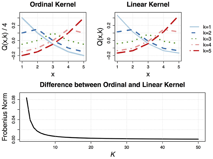
Figure 2. (Top) Visualization of the (standardized) ordinal and linear smoothing spline reproducing kernel functions with K = 5 levels of X. (Bottom) Frobenius norm between the (standardized) ordinal and linear smoothing spline reproducing kernel matrices Q as a function of K.
3.4. Approximation for Large K
If the number of elements of the ordered set K is quite large, then using all K levels as knots would be computationally costly. In such cases, the unconstrained ordinal smoothing spline solution can be fit via the formulas in Equations (14) and (16) with a set of knots . When monotonicity constraints are needed, the ordinal smoothing spline would still be computationally costly for large K. This is because the factorization of the reproducing kernel into the outer product of monotonic functions, i.e., Q = MM′, depends on K. For a scalable approximation to the ordinal smoothing spline isotonic regression estimator, the penalty functional itself can be approximated such as
where the knots are assumed to be ordered and unique. The modified RKHS is
for x ∈ {1, …, K} and j ∈ {2, …, R}. The modified RKHS has the modified inner product
where is a K × 1 vector that contains ones in the positions corresponding to the R knots and zeros elsewhere, and is a sparse R−1×K first order difference operator matrix with entries defined as
As an example, with K = 5 and R = 3 knots , the matrix has the form
Theorem 3.4. Given the ordinal smoothing spline inner-product in Equation (35), the null space has reproducing kernel ρ0(x, y) = 1/R, and the contrast space has reproducing kernel
for x, y ∈ {1, …, K} where 1{·} is an indicator function and are the knots.
See the Supplementary Material for a proof. Note that Theorem 3.4 provides the reproducing kernel needed to compute the ordinal smoothing spline isotonic regression estimator using the knot-based approximation for large K. Specifically, Theorem 3.4 reveals that we can write and where with for i = 1, …, n and j = 1, …, R − 1, and with for i = 1, …, R and j = 1, …, R − 1. Note that where is a selection matrix such that if xi = j = 1 or for j = 2, …, R, and otherwise. Using the modified reproducing kernel, the reparameterized ordinal smoothing spline problem is
where , so analogs of the results in Section 3.2 can be applied.
4. Simulation Study
To investigate the performance of the ordinal smoothing spline, we designed a simulation study that manipulated two conditions: (i) the sample size (4 levels: n ∈ {50, 100, 200, 500}), and (ii) the data generating function η (2 forms, see Figure 3). To simulate the data, we defined xi to be an equidistant sequence of n points spanning the interval [0,1], and then defined yi = η(xi) + ϵi where the error terms were (independently) randomly sampled from a standard normal distribution. Note that each xi is unique, so K = n in this case. We compared four different methods as a part of the simulation: (a) linear smoothing spline, (b) ordinal smoothing spline, (c) monotonicity constrained ordinal smoothing spline, and (d) isotonic regression implemented through the isoreg function in R [6]. Methods (a)–(c) were fit using the bigsplines package [41] in R. For the smoothing spline methods, we used the same sequence of 20 points as knots to ensure that differences in the results are not confounded by differences in the knot locations. For each of the 8 (4 n × 2 η) cells of the simulation design, we generated 100 independent samples of data and fit each of the four models to each generated sampled.
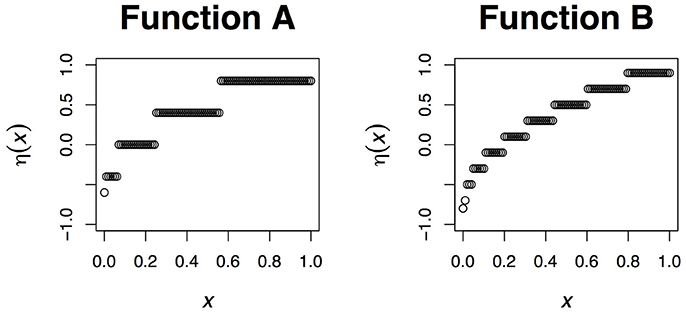
Figure 3. The data generating functions from the simulation study. In each case, the function is defined as where the are a sequence of equidistant knots spanning the interval [0,1].
To evaluate the performance of each method, we calculated the root mean squared error (RMSE) between the truth η and the estimate . The RMSE for each method is displayed in Table 2 and Figure 4, which clearly reveal the benefit of the ordinal smoothing spline. Specifically, Figure 4 reveals that the unconstrained ordinal smoothing spline outperforms the linear smoothing spline for smaller values of n = K, and performs similarly to linear smoothing spline for large values of K. Figure 4 also reveals that the monotonicity constrained estimator (using the knot-approximated reproducing kernel function described in Section 3.4) performed slightly better than the unconstrained ordinal smoothing spline, particularly in the n = 50 condition. Furthermore, the simulation results in Figure 4 demonstrate that the ordinal smoothing spline systematically outperforms R's (default) isotonic regression routine. Thus, the ordinal smoothing spline offers an effective alternative to classic nonparametric and isotonic regression approaches, and—unlike the linear smoothing spline—the ordinal smoothing spline has the benefit of being invariant to any monotonic transformation of x.
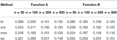
Table 2. Median root mean squared error (RMSE) across 100 simulation replications.
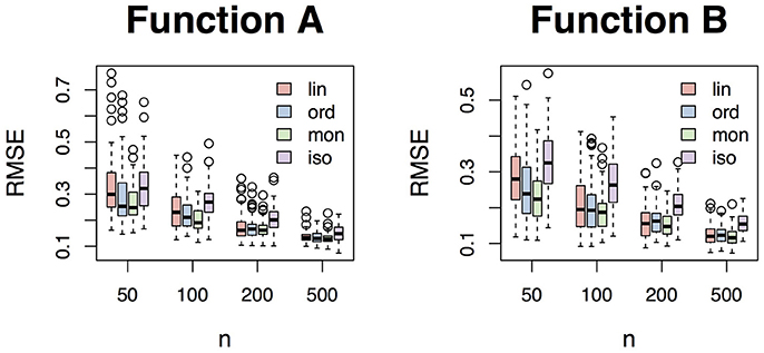
Figure 4. Box plots of the root mean squared error (RMSE) between η and for each method.
5. Examples
5.1. Example 1: Income by Education and Sex
To demonstrate the power of the monotonic ordinal smoothing spline, we use open source data to examine the relationship between income and educational attainment. The data were collected as a part of the 2014 US Census and are freely available from the Integrated Public Use Microdata Series (IPUMS) USA website (https://usa.ipums.org/usa/), which is managed by the Minnesota Population Center at the University of Minnesota. Note that the original data file usa_00001.dat contains data from n* = 3, 132, 610 subjects. However, we restrict our analyses to individuals who were 18+ years old and earned a non-zero income as reported on their 2014 census, resulting in a sample size of n = 2, 214, 350 subjects. We fit the monotonic ordinal smoothing spline separately to the males' data (n = 1, 093, 949) and females' data (n = 1, 120, 401) using all 11 unique education levels as knots. Due to the positive skewness of the income data, we fit the model to y = log(income). Finally, to ensure our results were nationally representative, we fit the model via weighted penalized least squares using the person weights (PERWT) provided with the IPUMS data.
The fit models explain about 15% of the variation in the male and female income data, and reveal noteworthy differences in expected incomes as a function of education and sex. The predicted mean incomes for each educational attainment level and sex are plotted in Figure 5, which has some striking trends. First, note that expected income is low (about $15,000 for males and $10,000 for females) for individuals without a high school education. Completing high school results in an approximate $7,000 expected increase in income for men, but only a $4,500 expected increase in income for women. Similarly, completing 1 year of college results in an expected $1,700 pay increase for men, but only an expected $1,000 increase for women. This disturbing trend continues to magnify at each education level, such that women receive a smaller expected return on their education. At the highest level of educational attainment, the gender pay gap is most pronounced such that women tend to make about $28,000 less per year than men.
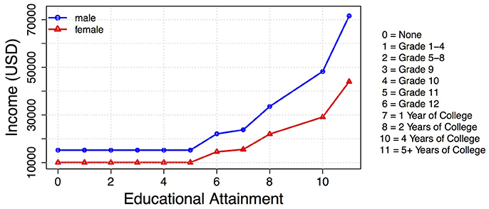
Figure 5. Monotonic ordinal smoothing spline solution showing the relationship between education and income for males (blue circle) and females (red triangle).
5.2. Example 2: Student Math Performance
As a second example, we use math performance data from Portuguese secondary students. The data were collected by Paulo Cortez at the University of Minho in Portugal [42], and are available from the UCI Machine Learning Repository [43]. In this example, we use the math performance data (student-mat.csv), which contains math exam scores from n = 395 Portuguese students. We focus on predicting the students' scores on the first exam during the period (G1). Unlike Cortez et al., we model the first exam (instead of the final grade) because we hope to identify factors that cause students to fall behind early in the semester. By discovering factors that relate to poor math performance on the first exam, it may be possible to create student-specific interventions (e.g., tutoring or more study time) with hopes of improving the final grade.
In Table 3, we describe the 15 predictor variables that we include in our model. To model the math exam scores, we fit a semiparametric regression model of the form
where mathi is the i-th student's score on the first math exam, β0 is an unknown regression intercept, (β1, …, β6) are unknown regression coefficients corresponding to the six binary predictors (school, sex, famsup, paid, activities, nursery), ηj is the j-th effect function for j = 1, …, 9, and is the i-th student's model error term. We used a cubic smoothing spline marginal reproducing kernel for the integer valued variables (age, failures, absences) because these variables are measured on a ratio scale. We used the ordinal smoothing spline reproducing kernel (see Theorem 3.1) for the other six nonparametric effects because these variables were measured on an ordinal scale (see Table 3). The full smoothing spline solution was fit, i.e., all n = 395 data points were used as knots.
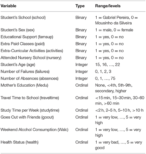
Table 3. Predictor variables for math performance example.
The smoothing parameters were chosen by minimizing the GCV criterion [35]. To avoid the computational expense of simultaneously tuning the GCV criterion with respect to 9 smoothing parameters (one for each ηj), we used a version of Algorithm 3.2 described by Gu and Wahba [25] to obtain initial values of the smoothing parameters. Then we fit the model with the 9 local smoothing parameters fixed at the initialized values, and optimized the GCV criterion with respect to the global smoothing parameter λ. This approach has been shown to produce results that are essentially identical to the fully optimal solution (see [15, 26]).
The fit model explains about 23% of the variation in the students' scores on the first math exam. The estimated regression coefficients and effect functions are plotted in Figure 6, along with 90% Bayesian confidence intervals [37, 38, 40] around the effect functions. Examining the top row of Figure 6, it is evident that only two of the six parametric effects has a significant effect: sex and famsup. The signs and magnitudes of these significant coefficients reveal that (i) males tend to get higher math exam scores than females, and (ii) students who receive extra educational support from their families tend to get lower math exam scores. This second point may seem counter-intuitive, because one may think that extra educational support should lead to higher grades. However, it is likely that the students who receive extra support are receiving this extra support for a reason.
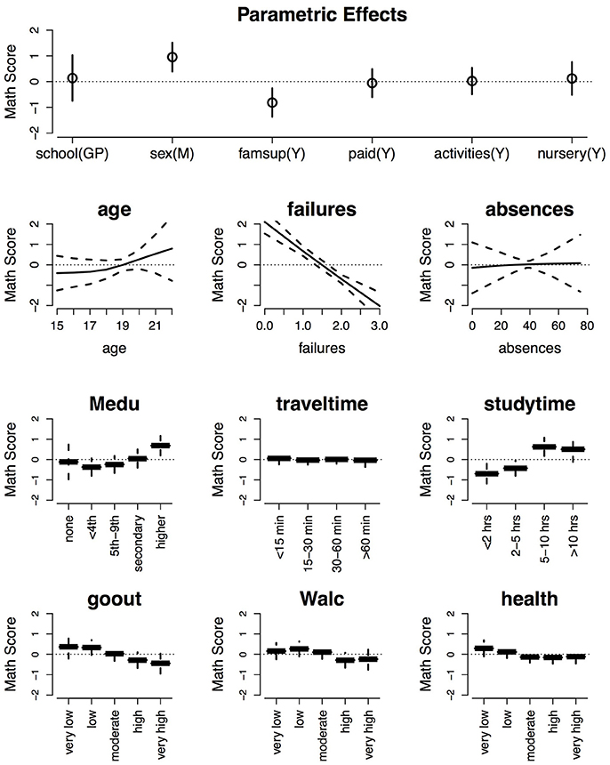
Figure 6. Estimated effects of the different predictor variables on expected math scores with 90% Bayesian confidence intervals (dashed lines) around the predictions.
Examination of the remaining subplots in Figure 6 reveals that the number of prior course failures has the largest (negative) effect on the expected math scores, which is not surprising. There is a slight trend such that larger ages lead to better grades, but the trend is not significantly different from zero according to the 90% Bayesian confidence intervals. Given the other effects in the model, the number of absences has no effect on the expected math scores, which is surprising. Having a mother who completed higher education increases a student's expected math exam score, whereas there were no significant differences between the other four lesser levels of the mother's education. Studying for 5 or more hours per week increases a student's expected scores, whereas studying less than 2 h per week decreases a student's expected scores. Going out with friends and/or drinking on the weekend with high or very high frequency significantly decreases a student's expected math exam scores. Given the other effects, travel time to school and a student's health did not have significant effects on the math exam scores.
6. Discussion
6.1. Summary of Findings
Our simulation and real data examples reveal the flexibility and practical potential of the ordinal smoothing spline. The simulation study investigated the potential of the ordinal smoothing spline for isotonic regression, as well as the relationship between the ordinal and linear smoothing spline reproducing kernel functions. The simulation results demonstrated that (i) the ordinal smoothing spline can outperform the linear smoothing spline at small samples, (ii) the ordinal smoothing spline performs similar to the linear smoothing spline for large K, and (iii) monotonic ordinal smoothing splines can outperform standard isotonic regression approaches. Thus, the simulation study illustrates the results in Theorems 3.1–3.3, and also reveals that the knot-approximated reproducing kernel proposed in Theorem 3.4 offers an effective approximation to the monotonic ordinal smoothing spline solution.
The first example (income by education and sex) offers a practical example of the potential of the ordinal smoothing spline for discovering monotonic trends in data. Unlike classic approaches to isotonic regression, the ordinal smoothing spline uses a reproducing kernel (and knot-based) approach, making it easily scalable to large survey samples such as the US Census data. Using a large and nationally representative sample of US citizens ages 18+, this example reveals a clear gender pay gap, such that women receive less return on their educational investments, i.e., less pay for the same level of education. And note that the predictor could be monotonically transformed without changing the ordinal smoothing spline solution, which is one of the primary benefits of using the ordinal smoothing spline estimator for variables such as Educational Attainment—which has no clear unit of measurement.
The second example (math grades) demonstrates the effectiveness of using ordinal smoothing splines to include multiple ordinal predictors in a regression model along with other nominal and metric (continuous) predictors. Furthermore, the second example illustrates that many ordinal relationships do not have a clear linear in/decrease across the K levels of the ordinal variable. This reveals that it could be difficult and/or misleading to code ordinal predictors as if they were continuous (e.g., linear) effects. So, despite this common practice in the social sciences, our results make it clear that this sort of approach does not have an obvious solution for all ordinal variables, and could be particularly problematic when multiple ordinal variables are included in the same model.
6.2. Concluding Remarks
This paper discusses the ordinal smoothing spline, which can be used to model functional relationships between ordered categorical predictor variables and any exponential family response variable. This approach makes it straightforward to incorporate one (or more) ordinal predictors in a regression model, and also provides a theoretically sound method for examining interaction effects between ordinal and other predictors. In this paper, we present the ordinal smoothing spline reproducing kernel function (Theorem 3.1), which has the benefit of being invariant to any monotonic transformation of the predictor. We also discuss how the ordinal smoothing spline estimator can be adjusted to impose monotonicity constraints (Theorem 3.2). Furthermore, we reveal an interesting asymptotic relationship between ordinal and linear smoothing splines (Theorem 3.3), and develop large sample approximations for ordinal smoothing splines (Theorem 3.4). Finally, we have demonstrated the practical potential of ordinal smoothing splines using a simulation study (Section 4) and real data examples from two distinct disciplines (Section 5).
In nearly all applications of the GLM or GzLM, ordered categorical predictors are treated as either unordered categorical predictors or metric predictors for modeling purposes. In most cases, it is not obvious which approach one should choose. Neither approach is ideal for ordinal data, so one must ultimately decide which aspect of the data should be misrepresented in the model. Treating ordinal data as unordered (by definition) ignores the ordinal nature of the data, which is undesirable. Whereas, treating ordinal data as metric (continuous) ignores the discrete nature of the data, which is undesirable. In contrast, the ordinal smoothing spline is the obvious solution to this problem, because the ordinal smoothing spline (i) respects the ordinal nature of the predictor, and (ii) provides a theoretically sound framework for incorporating ordinal predictors in regression models.
Author Contributions
The sole author (NH) contributed to all aspects of this work.
Funding
The sole author (NH) was funded by start-up funds from the University of Minnesota.
Conflict of Interest Statement
The author declares that the research was conducted in the absence of any commercial or financial relationships that could be construed as a potential conflict of interest.
Acknowledgments
The author acknowledges the two data sources: (i) the Minnesota Population Center at the University of Minnesota, and (ii) the Machine Learning Repository at University of California Irvine.
Supplementary Material
The Supplementary Material for this article can be found online at: https://www.frontiersin.org/article/10.3389/fams.2017.00015/full#supplementary-material
References
1. Christensen R. Plane Answers to Complex Questions: The Theory of Linear Models. 3rd Edn. New York, NY: Springer-Verlag (2002).
2. Chartier S, Faulkner A. General linear models: an integrated approach to statistics. Tutorial Quant Methods Psychol. (2008) 4:65–78. doi: 10.20982/tqmp.04.2.p065
3. Graham JM. The general linear model as structural equation modeling. J Educ Behav Stat. (2008) 33:485–506. doi: 10.3102/1076998607306151
4. Casals M, Girabent-Farrés M, Carrasco JL. Methodological quality and reporting of generalized linear mixed models in clinical medicine (2000–2012): a systematic review. PLoS ONE (2014) 9:e112653. doi: 10.1371/journal.pone.0112653
5. de Jong P, Heller GZ. Generalized Linear Models for Insurance Data. Cambridge: Cambridge University Press (2008).
6. R Core Team. R: A Language Environment for Statistical Computing. Vienna (2017). Available online at: http://www.R-project.org/
8. McCullagh P. Regression model for ordinal data (with discussion). J R Stat Soc Ser B (1980) 42:109–42.
9. Armstrong B, Sloan M. Ordinal regression models for epidemiologic data. Am J Epidemiol. (1989) 129:191–204. doi: 10.1093/oxfordjournals.aje.a115109
10. Peterson B, Harrell FE Jr. Partial proportional odds models for ordinal response variables. J R Stat Soc Ser C (1990) 39:205–17. doi: 10.2307/2347760
11. Cox C. Location-scale cumulative odds models for ordinal data: a generalized non-linear model approach. Stat Med. (1995) 14:1191–203. doi: 10.1002/sim.4780141105
12. Liu I, Agresti A. The analysis of ordinal categorical data: an overview and a survey of recent developments. Test (2005) 14:1–73. doi: 10.1007/BF02595397
13. Gertheiss J, Tutz G. Penalized regression with ordinal predictors. Int Stat Rev. (2009) 77:345–65. doi: 10.1111/j.1751-5823.2009.00088.x
14. Gertheiss J. ordPens: Selection and/or Smoothing of Ordinal Predictors. R package version 0.3-1 (2015). Available online at: https://CRAN.R-project.org/package=ordPens
15. Gu C. Smoothing Spline ANOVA Models. 2nd Edn. New York, NY: Springer-Verlag (2013). doi: 10.1007/978-1-4614-5369-7
16. Wahba G. Spline Models for Observational Data. Philadelphia, PA: Society for Industrial and Applied Mathematics (1990).
17. Riesz F. Sur une espèce de géométrie analytique des systèmes de fonctions sommables. C R Acad Sci Paris (1907) 144:1409–11.
19. Aronszajn N. Theory of reproducing kernels. Trans Am Math Soc. (1950) 68:337–404. doi: 10.1090/S0002-9947-1950-0051437-7
20. Ruppert D, Wand MP, Carroll RJ. Semiparametric Regression. Cambridge: Cambridge University Press (2003).
23. Wood SN. Generalized Additive Models: An Introduction with R. Boca Raton, FL: Chapman & Hall (2006).
24. Kimeldorf G, Wahba G. Some results on Tchebycheffian spline functions. J Math Anal Appl. (1971) 33:82–95. doi: 10.1016/0022-247X(71)90184-3
25. Gu C, Wahba G. Minimizing GCV/GML scores with multiple smoothing parameters via the Newton method. SIAM J Sci Stat Comput. (1991) 12:383–98. doi: 10.1137/0912021
26. Helwig NE, Ma P. Fast and stable multiple smoothing parameter selection in smoothing spline analysis of variance models with large samples. J Comput Graph Stat. (2015) 24:715–32. doi: 10.1080/10618600.2014.926819
27. Duchon J. Splines minimizing rotation-invariant semi-norms in Sobolev spaces. In Schempp W, Zeller K editors. Constructive Theory of Functions of Several Variables. Lecture Notes in Mathematics, Vol. 571. Berlin; Heidelberg: Springer (1977). p. 85–100.
28. Meinguet J. Multivariate interpolation at arbitrary points Made simple. J Appl Math Phys. (1979) 30:292–304. doi: 10.1007/BF01601941
29. Wood SN. Thin plate regression splines. J R Stat Soc Ser B (2003) 65:95–114. doi: 10.1111/1467-9868.00374
30. Gu C, Kim YJ. Penalized likelihood regression: general formulation and efficient approximation. Can J Stat. (2002) 30:619–28. doi: 10.2307/3316100
31. Kim YJ, Gu C. Smoothing spline Gaussian regression: more scalable computation via efficient approximation. J R Stat Soc Ser B (2004) 66:337–56. doi: 10.1046/j.1369-7412.2003.05316.x
32. Helwig NE, Ma P. Smoothing spline ANOVA for super-large samples: scalable computation via rounding parameters. Stat Its Interface (2016) 9:433–44. doi: 10.4310/SII.2016.v9.n4.a3
34. Penrose R. A generalized inverse for matrices. Math Proc Cambridge Philos Soc. (1950) 51:406–13. doi: 10.1017/S0305004100030401
35. Craven P, Wahba G. Smoothing noisy data with spline functions: estimating the correct degree of smoothing by the method of generalized cross-validation. Numerische Mathematik (1979) 31:377–403. doi: 10.1007/BF01404567
36. Kimeldorf G, Wahba G. A correspondence between Bayesian estimation on stochastic processes and smoothing by splines. Ann Math Stat. (1970) 41:495–502. doi: 10.1214/aoms/1177697089
37. Wahba G. Bayesian “confidence intervals” for the cross-validated smoothing spline. J R Stat Soc Ser B (1983) 45:133–50.
38. Nychka D. Bayesian confidence intervals for smoothing splines. J Am Stat Assoc. (1988) 83:1134–43. doi: 10.1080/01621459.1988.10478711
40. Gu C, Wahba G. Smoothing spline ANOVA with component-wise Bayesian “confidence intervals”. J Comput Graph Stat. (1993) 2:97–117.
41. Helwig NE. Bigsplines: Smoothing Splines for Large Samples. R package version 1.1-0 (2017). Available online at: http://CRAN.R-project.org/package=bigsplines
42. Cortez P, Silva A. Using data mining to predict secondary school student performance. In Brito A, Teixeira J editors. Proceedings of 5th FUture BUsiness TEChnology Conference (FUBUTEC 2008). Porto: EUROSIS (2008). p. 5–12.
43. Lichman M. UCI Machine Learning Repository. (2013). Available online at: http://archive.ics.uci.edu/ml
Keywords: isotonic regression, monotonic regression, nonparametric regression, ordinal data, smoothing spline, step function
Citation: Helwig NE (2017) Regression with Ordered Predictors via Ordinal Smoothing Splines. Front. Appl. Math. Stat. 3:15. doi: 10.3389/fams.2017.00015
Received: 02 May 2017; Accepted: 12 July 2017;
Published: 28 July 2017.
Edited by:
Sou Cheng Choi, Illinois Institute of Technology, United StatesReviewed by:
Katerina Hlavackova-Schindler, University of Vienna, AustriaJunhui Wang, City University of Hong Kong, Hong Kong
Copyright © 2017 Helwig. This is an open-access article distributed under the terms of the Creative Commons Attribution License (CC BY). The use, distribution or reproduction in other forums is permitted, provided the original author(s) or licensor are credited and that the original publication in this journal is cited, in accordance with accepted academic practice. No use, distribution or reproduction is permitted which does not comply with these terms.
*Correspondence: Nathaniel E. Helwig, helwig@umn.edu