Investigating (re)current state-of-the-art in human activity recognition datasets
 Marius Bock
 Alexander Hoelzemann
 Michael Moeller1
  Kristof Van Laerhoven
- 1Computer Vision, Department of Electrical Engineering and Computer Science, University of Siegen, Siegen, Germany
- 2Ubiquitous Computing, Department of Electrical Engineering and Computer Science, University of Siegen, Siegen, Germany
Many human activities consist of physical gestures that tend to be performed in certain sequences. Wearable inertial sensor data have as a consequence been employed to automatically detect human activities, lately predominantly with deep learning methods. This article focuses on the necessity of recurrent layers—more specifically Long Short-Term Memory (LSTM) layers—in common Deep Learning architectures for Human Activity Recognition (HAR). Our experimental pipeline investigates the effects of employing none, one, or two LSTM layers, as well as different layers' sizes, within the popular DeepConvLSTM architecture. We evaluate the architecture's performance on five well-known activity recognition datasets and provide an in-depth analysis of the per-class results, showing trends which type of activities or datasets profit the most from the removal of LSTM layers. For 4 out of 5 datasets, an altered architecture with one LSTM layer produces the best prediction results. In our previous work we already investigated the impact of a 2-layered LSTM when dealing with sequential activity data. Extending upon this, we now propose a metric, rGP, which aims to measure the effectiveness of learned temporal patterns for a dataset and can be used as a decision metric whether to include recurrent layers into a network at all. Even for datasets including activities without explicit temporal processes, the rGP can be high, suggesting that temporal patterns were learned, and consequently convolutional networks are being outperformed by networks including recurrent layers. We conclude this article by putting forward the question to what degree popular HAR datasets contain unwanted temporal dependencies, which if not taken care of, can benefit networks in achieving high benchmark scores and give a false sense of overall generability to a real-world setting.
1. Introduction
Research in activity recognition has early on recognized the importance of capturing temporal dependencies in sensor-based data with early approaches using classical generative Machine Learning algorithms in order to do so (e.g., Lester et al., 2005). With the advancement of Deep Learning—becoming the de facto standard in sensor-based Human Activity Recognition (HAR)—approaches shifted to using Recurrent Neural Networks (RNNs) (e.g., Hammerla et al., 2016), Long-Short-Term Memory networks (LSTMs) (e.g., Edel and Köppe, 2016) and Transformers (e.g., Dirgová Luptáková et al., 2022). Based on findings presented in Jaakkola and Haussler (1998), early works already demonstrated the effectiveness of combining both discriminative and generative models (Lester et al., 2005). Within the area of Deep Learning, the combination of convolutional (discrimnative) and recurrent (generative) layers saw particular success, with the DeepConvLSTM (Ordóñez and Roggen, 2016) being the first architecture to take advantage of the capabilities of both types of layers. The architecture achieved state-of-the-art results on both the Opportunity challenge (Roggen et al., 2010) and Skoda Mini Checkpoint dataset (Zappi et al., 2008).
After Ordóñez and Roggen (2016) introduced us to the DeepConvLSTM, Hammerla et al. (2016) analyzed the effectiveness of the RNNs as well as their combination with convolutional layers and came to the conclusion that whether RNNs are beneficial and increase prediction performance is dependent on the nature of activities and dataset itself. The original DeepConvLSTM (Ordóñez and Roggen, 2016) architecture features a 2-layered LSTM with 128 hidden units. In Bock et al. (2021) we demonstrated that altering the DeepConvLSTM to employ a 1-layered instead of a 2-layered LSTM not only heavily decreases training time, but also significantly increases prediction performance across 5 popular HAR datasets (Roggen et al., 2010; Scholl et al., 2015; Stisen et al., 2015; Reyes-Ortiz et al., 2016; Sztyler and Stuckenschmidt, 2016). Our findings stood in contrast to the belief that one needs at least a 2-layered LSTM when dealing with sequential data (Karpathy et al., 2015). In this article we want to extend upon the work conducted by Hammerla et al. (2016) by putting it into context with what we found out in Bock et al. (2021). Unlike Hammerla et al. (2016) we use a larger variety of datasets with different types of activities and fix all parts of the training process across experiments to ensure that changes in predictive performance can be accredited to changes to the recurrent parts of the network. Furthermore, we want to go one step further by questioning the necessity of recurrent layers in sensor-based HAR altogether and introduce a second variation of the DeepConvLSTM (Ordóñez and Roggen, 2016) which has all LSTM layers removed. We include said variation into the experimental workflow we illustrated in Bock et al. (2021).
Our article's contributions are threefold:
1. We provide an in-depth analysis of the performance of the DeepConvLSTM (Ordóñez and Roggen, 2016), as well as two variations of it, on 5 popular HAR datasets (Roggen et al., 2010; Scholl et al., 2015; Stisen et al., 2015; Reyes-Ortiz et al., 2016; Sztyler and Stuckenschmidt, 2016), showing trends in which types of activities or datasets benefit the most from the removal of LSTM layers.
2. We propose a correlation factor rGP which can measure the effectiveness of learned temporal patterns and which can be used as guidance to whether inclusion of recurrent layers into a Deep Learning architecture for a given HAR dataset can be predicted to be helpful.
3. Based on our findings, we extend upon our claims in Bock et al. (2021) and argue that larger LSTMs are more likely to overfit on temporal patterns of a dataset, which, depending on the use case, might end up hurting generability of trained models to a real-world setting.
2. Related work
The predictive performance of classical Machine Learning approaches highly relies on sophisticated, handcrafted features (Pouyanfar et al., 2018). In the last decade, Deep Learning has shown to outperform classical Machine Learning algorithms in many areas, e.g., image recognition (Farabet et al., 2013; Tompson et al., 2014; Szegedy et al., 2015), speech recognition (Mikolov et al., 2011; Hinton et al., 2012; Krizhevsky et al., 2012; Sainath et al., 2013) and Natural Language Processing (Collobert et al., 2011; Bordes et al., 2014; Jean et al., 2014; Sutskever et al., 2014). Much of this success can be accredited to the fact that Deep Learning does not require manual feature engineering, but is able to automatically extract discriminative features from raw data input (Najafabadi et al., 2015). The advantage of being able to apply algorithms on raw data and not being dependent on handcrafted features has led to studies investigating the effectiveness of Deep Learning in HAR, which e.g., suggested different architectures (Ordóñez and Roggen, 2016), evaluated the generality of architectures (Hammerla et al., 2016) and assessed the applicability in real-world scenarios (Guan and Plötz, 2017).
Research in activity recognition has early on recognized the importance of capturing temporal regularities and dependencies in sensor-based data (Lester et al., 2005). Early approaches involved using classical generative Machine Learning algorithms such as Hidden Markov Models (Lester et al., 2005, 2006; Patterson et al., 2005; van Kasteren et al., 2008; Reddy et al., 2010), Conditional Random Fields (Liao et al., 2005; van Kasteren et al., 2008) or Bayesian networks (Patterson et al., 2005). With the advancement of Deep Learning methods like Recurrent Neural Networks (RNNs) (Hammerla et al., 2016; Inoue et al., 2018), Long-Short-Term Memory (LSTM) networks (Edel and Köppe, 2016; Ordóñez and Roggen, 2016), Gated Recurrent Units (GRUs) (Xu et al., 2019; Abedin et al., 2021; Dua et al., 2021) and Transformers (Haresamudram et al., 2020; Dirgová Luptáková et al., 2022) became the de facto standard when trying to model temporal dependencies.
Based on the work of Jaakkola and Haussler (1998) and Lester et al. (2005) suggested to combine both generative and discriminative models in order to overcome weaknesses of the generative models in the context of HAR. More recently (Ordóñez and Roggen, 2016) introduced the DeepConvLSTM, a deep learning architecture which is a hybrid model combining both convolutional and recurrent layers. Similar to Lester et al. (2005) and Ordóñez and Roggen (2016) claim that by combining both types of layers the network is able to automatically extract discriminative features and model temporal dependencies. Extending up on the work of Ordóñez and Roggen (2016), researchers proposed variations of the DeepConvLSTM e.g., by appending attention layers to the original architecture (Murahari and Plötz, 2018) or adding dilated convolution layers in addition to normal convolution layers (Xi et al., 2018). Other publications followed up on the idea of combining convolutional and recurrent layers proposing their own architectures, e.g., combining Inception modules and GRUs (Xu et al., 2019), self-attention mechanisms and GRUs (Abedin et al., 2021) or having two ConvLSTM networks handling different time lengths to analyze more complex temporal hierarchies (Yuki et al., 2018).
Upon the experiments conducted by Karpathy et al. (2015) and Chen et al. (2021) claim within their recent survey paper on Deep Learning for HAR that “the depth of an effective LSTM-based RNN needs to be at least two when processing sequential data.” Within our recent publication we investigated the effect of employing a 1-layered instead of a 2-layered LSTM within the DeepConvLSTM architecture (Bock et al., 2021). As Karpathy et al. (2015) obtained their results using character-level language models, i.e., text data, our paper aimed at challenging the belief that their claim is applicable to sensor-based HAR. With this publication we want to go one step further in analyzing the necessity of recurrent layers in HAR altogether by completely removing the LSTM, and thus all recurrent layers, from the DeepConvLSTM (Ordóñez and Roggen, 2016). Our analysis is most similar to the one conducted by Hammerla et al. (2016) which compared Deep Neural Networks (DNNs) against CNNs, RNNs and, as a combination of both, the DeepConvLSTM (Ordóñez and Roggen, 2016). Hammerla et al. (2016) based their analysis on three datasets namely the Physical Activity Montioring (PAMAP2) (Reiss and Stricker, 2012), the Daphnet Freezing of Gait (Bachlin et al., 2009) and the Opportunity challenge (Roggen et al., 2010) dataset. Hammerla et al. (2016) concluded that RNNs are beneficial and increase prediction performance for activities that are short in duration and have a natural ordering, while for movement data which focuses on short-term changes in patterns CNNs are a better option. Unlike Hammerla et al. (2016) we additionally analyze datasets which include complex (Scholl et al., 2015) and transitional activities (Reyes-Ortiz et al., 2016) as well as datasets which were recorded in a naturalistic environment (Scholl et al., 2015; Stisen et al., 2015; Sztyler and Stuckenschmidt, 2016). Furthermore, we made sure to use the same hyperparameters across all experiments to give every variation the same starting point. This way we want to ensure that differences in performance can be singled down to changes in the recurrent layers.
3. Methodology
Contrary to the belief that one needs at least a two-layered LSTM when dealing with sequential data Karpathy et al. (2015) and Bock et al. (2021) we proposed to change the DeepConvLSTM to employ a one-layered LSTM. Extending upon these experiments we now want to investigate the overall necessity of recurrent layers in HAR and therefore additionally evaluate the performance of an altered DeepConvLSTM architecture which has the LSTM completly removed. Figure 2 illustrates the evaluated architecture changes.
3.1. Datasets
We evaluated our architecture changes using five popular HAR datasets, namely the Wetlab (Scholl et al., 2015), the RealWorld HAR (RWHAR) (Sztyler and Stuckenschmidt, 2016), the Smartphone-Based Recognition of Human Activities and Postural Transitions (SBHAR) (Reyes-Ortiz et al., 2016), the Heterogeneity Activity Recognition (HHAR) (Stisen et al., 2015) and the Opportunity (Roggen et al., 2010) dataset. To ensure that our assessment on the necessity of recurrent layers in HAR is not biased toward specific traits of a dataset, we made sure to use a variety of different datasets which differ in the type of activities being performed and circumstances under which the data was recorded. Activity-wise we differentiate between sporadic, simple/ periodical, transitional and complex activities. Sporadic activities, e.g., opening a door, are short in time and do not contain any reoccurring patterns within their execution. Contrarily, simple/ periodical activities, e.g., walking, are (usually) longer in time of execution and tend to contain subject-independent, periodical patterns in the sensor data. Transitional activities as seen for example in the SBHAR dataset (Reyes-Ortiz et al., 2016) mark the period in-between two activities, e.g., the period from lying down to standing up. Similar to sporadic activities they are (usually) short in time and do not contain any reoccurring patterns within their execution. Complex activities, e.g., making a coffee, are activities which are composed of more than one sub-activities, which itself can be either sporadic, simple/ periodical or transitional. In order to further investigate the overall shape of a dataset we created color-coded plots along with the sensor data indicating which parts of a dataset are accredited to which activity and subject (see e.g., Figure 1 for an illustration of the HHAR dataset Stisen et al., 2015). This allows us to better analyze and judge the degree of repetition, rapid changes and distribution of data among subjects within each dataset. We did not include all plots within this article, but advise readers to recreate the plots themselves using a script we provide in our repository1 as it allows to better zoom in and out without loss of readability.
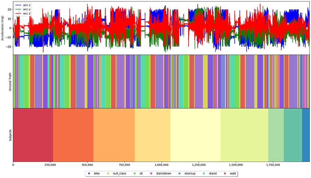
Figure 1. Plotted 3D-acceleration data of the HHAR dataset (Stisen et al., 2015) along with color-coded bitmaps indicating which part of the sensor stream belongs to which activity and which subject. This type of plot can be recreated for every dataset using a script we provide in our repository (https://github.com/mariusbock/recurrent_state_of_the_art) and was used as basis for our analysis of each dataset.
For the Wetlab (Scholl et al., 2015), RWHAR (Sztyler and Stuckenschmidt, 2016), SBHAR (Reyes-Ortiz et al., 2016), and HHAR dataset (Stisen et al., 2015) we limited ourselves to only use 3D-acceleration data of a sensor—if possible—located on the right wrist of the subject. For the Opportunity dataset (Roggen et al., 2010) many sensors exhibited packet loss. We therefore chose to use the same sensors as Ordóñez and Roggen (2016) to reduce the effect of missing values. In the following, each dataset, its type of activities and limitations will be explained in more detail.
3.1.1. Wetlab
The Wetlab dataset (Scholl et al., 2015) consists of 22 subjects performing two DNA extraction experiments within a wetlab environment and provides two types of annotations namely tasks and actions. While the former are specific steps within the experimental protocol, the latter represents underlying activities. As the experiments followed an experimental protocol, recording sessions of different subjects contain almost identical sequences of consecutive activities. Nevertheless, it should also be noted that some activities were not performed for some subjects as not all steps in the protocol were not mandatory and were therefore sometimes skipped by subjects. Within our experiments we predicted the annotated actions which left us with 8 different classes, namely cutting, inverting, peeling, pestling, pipetting, pouring, stirring and transfer as well as a null class. In total the dataset consists of 18 h of collected data. As each subject performed the experiment in their own time, execution times per subject differ and average execution times per activity vary greatly, lasting between half a second up to three and a half minutes. Furthermore, the class distribution is imbalanced with the null class having almost ten-times as many instances as the longest recorded activity (pestling). While performing the activities 3D-accelerometer data of the dominant wrist of each subject was recorded at 50Hz. Activities contained in the Wetlab dataset can be classified as both simple/ periodical (e.g., stirring) and complex activities (e.g., cutting).
3.1.2. RWHAR
The RWHAR dataset consists of 15 subjects performing a set of 8 different simple/ periodical activities (Sztyler and Stuckenschmidt, 2016). The activities are climbing_down, climbing_up, jumping, lying, standing, sitting, running and walking. The dataset was collected in a real-world scenario, i.e., with participants not performing the activities in a controlled lab environment, but at different locations like their own home or in public places. In total the dataset consists of roughly 18 h of data (1 h per subject), with activities not always being recorded in the same order for each subject. Due to the fact that each activity was recorded in sessions, i.e., having participants perform a single activity for a certain amount of time, the average activity lengths (except for the activity jumping, climbing_down and climbing_up) are around 10 min without any recurrences and rapid changes of activities. Though the dataset offers many different sensors, we chose to use 3D-acceleration data captured by a sensor attached to the right wrist, which was set to sample at 50Hz.
3.1.3. SBHAR
The SBHAR dataset consists of 30 subjects performing 6 activities of daily living (standing, sitting, lying, walking, walking downstairs walking upstairs) (Reyes-Ortiz et al., 2016). In addition to the 6 simple/ periodical activities, 6 transitional activities (stand-to-sit, sit-to-stand, sit-to-lie, lie-to-sit, stand-to-lie and lie-to-stand) along with a null class are also annotated in the data. The dataset contains roughly 6 h of recorded data (between 10 and 15 min per subject) and was collected in a controlled lab environment. During experiments subjects had to follow an experimental protocol which defined the order and length in which activities were to be performed. Labels are therefore fairly evenly distributed among the 6 simple/ periodical and 6 transitional activities, but are dominated by the (Sztyler and Stuckenschmidt, 2016), the SBHAR dataset (Reyes-Ortiz et al., 2016) has participants more rapidly change activities with the average execution time of the periodical/ simple activities being around 10–20 s and the transitional activities being around 2–5 s. Additionally, activities were executed multiple times and thus reooccur within each subject's data. Note that the smartphone, which was used for data collection sampling at 50Hz, was attached to the waist of the subjects.
3.1.4. HHAR
The HHAR dataset consists of 9 subjects performing 6 activities of daily living (biking, sitting, standing, walking, walking upstairs and walking downstairs) (Stisen et al., 2015). During experiments subjects were asked to perform each simple/ periodical activity for 5 min following a specific activity sequence, which also makes the class distribution fairly balanced amongst all classes. In total the dataset contains 5 h and 30 min of recorded data with the data being evenly distributed among the first 6 subjects (between 45 and 60 min). For subjects 7, 8, and 9 significantly less data is recorded (17, 20 and 8 min). Similar to the SBHAR dataset (Reyes-Ortiz et al., 2016), activities within the HHAR dataset (Stisen et al., 2015) were not recorded as a whole, but included breaks, i.e., periods of null class, and changes. Nevertheless, on average activities were executed for longer periods being around 20–30 s for the activites walking upstairs and walking downstairs and the null class and around 90–120 s for all other activites. The dataset was recorded in a controlled, real-world scenario with each activity being executed in two environments and routes. For our experiments we use 3D-acceleration data recorded by smartwatches worn by each subject. Unfortunately, the dataset does not state whether sensors were worn on the same wrist for all subjects. Furthermore, due to the fact that two types of smartwatches were used throughout experiments, sampling rates differed across experiments (100 or 200Hz). We therefore downsampled the data of the higher sampling smartwatches to be 100Hz as well. Additionally, we omitted faulty recording sessions which had only one sample.
3.1.5. Opportunity
The Opportunity dataset (Roggen et al., 2010) consists of 4 subjects performing activities of daily living. Similar to the Wetlab dataset (Roggen et al., 2010), the Opportunity dataset (Scholl et al., 2015) provides two types of annotations namely modes of locomotion and gestures. We used the latter during our experiments which left us with 18 classes which needed to be predicted. The activities were opening and closing door 1 and 2, fridge, dishwasher and drawers 1, 2 and 3, cleaning table, drinking from cup and toggling switch as well as a null class. Each subject performed 6 different recording sessions. 5 of these recording sessions were non-scripted (ADL runs), while one required subjects to repeat a sequence of the relevant 17 activities 20 times (Drill runs). The Opportunity dataset was recorded in an controlled, experimental environment. Roggen et al. (2010) state that during the ADL sessions, subjects were asked to follow a higher level protocol, but were allowed to interleave their actions along the way. In total the dataset contains 8 h of recorded activity time with roughly 2 h per subject. For each activity there is around 1–3 min of data per subject. Only the null class (1:30 h) and the activity drinking from cup (between 5 and 10 min) were recorded longer per subject. Average execution times are short, given that the dataset contains almost solely sporadic activities, being around 2–6 s per activity. Similar to the SBHAR and HHAR dataset, both session types had participants frequently switch between activities, therefore causing activities to reoccur within each recording session. As the body-worn sensor streams contain missing values due to packet loss, we decided to use the same set of sensor channels as Ordóñez and Roggen (2016) which left us with a dataframe consisting of in total 113 feature channels, each representing an individual sensor axis sampled at 30Hz. Unlike Ordóñez and Roggen (2016) we do not apply the train-test split as defined by the Opportunity challenge, but split the data subject-wise in order to perform Leave-One-Subject-Out (LOSO) cross-validation. Gestures contained in the Opportunity dataset can all be classified as sporadic activities, except for the activity cleaning table which can also be seen as a simple/ periodical activity.
3.2. Training
We chose to use the popular DeepConvLSTM architecture as introduced by Ordóñez and Roggen (2016) to base our assessment on. By combining both convolutional and recurrent layers, Ordóñez and Roggen (2016) claim that the network is able to automatically extract discriminative features and model temporal dependencies. We argue that the latter might not be necessary depending on the nature of the activities one tries to predict. We therefore compare predictive performance of the original DeepConvLSTM architecture against two variations of it. The first variation only features a 1-layered LSTM instead of a 2-layered LSTM. We already demonstrated that said change increases the overall predictive performance of the network (Bock et al., 2021). In addition to the 1-layered variant of the network, we now go one step further by completely removing the LSTM from the network, consequently cutting out all recurrent layers in the network. For the two architectures which include LSTM layers, we additionally evaluate settings where we vary the amount of hidden units employed in each layer, i.e., 128, 256, 512 and 1,024, which leaves us with 9 different architectures to be evaluated. Figure 2 illustrates the original DeepConvLSTM as well the two altered versions of the architecture.
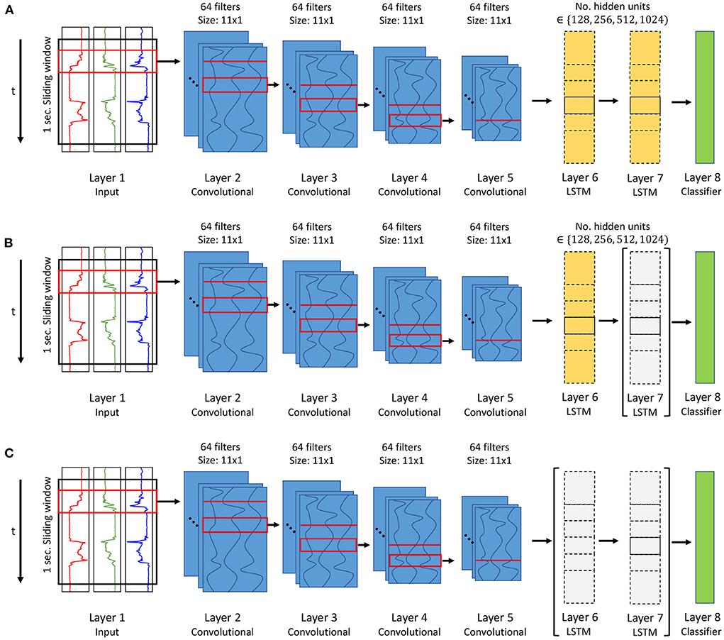
Figure 2. Illustration of the 3 evaluated architectures, namely (A) the original DeepConvLSTM architecture (Ordóñez and Roggen, 2016), (B) an altered version with a 1-layered LSTM (Layer 7 removed) (Bock et al., 2021) and (C) one with all LSTM layers (Layer 6 and 7) being removed. For (A,B) we vary the amount of hidden units within the LSTM layers to be either 128, 256, 512, or 1,024.
In general, we only modify the LSTM within the DeepConvLSTM architecture and other architecture specifications, i.e., dropout rate (0.5), number of convolution layers (4) and kernels per layer (64), are left unchanged to the original architecture (Ordóñez and Roggen, 2016). To minimize the effect of statistical variance, we train each architecture variation 5 times on each dataset, each time employing a different random seed drawn from a predefined set of 5 random seeds. We calculate the predictive performance of each architecture variation as the average performance results of said 5 runs. We chose to use the same hyperparameters as illustrated in Bock et al. (2021) which were obtained by evaluating multiple settings on the Wetlab dataset. As with our previous analysis (Bock et al., 2021) we again did not perform any hypertuning specific to the other datasets as we argue that our analysis is solely focused on the architectural changes and their influence on the predictive performance. We employed a sliding window approach with a window size of 1 s and an overlap of 60%. Furthermore we used the Adam optimizer with a weight decay of 1e−6 and a constant learning rate of 1e−4 and initialized weights using the Glorot initialization (Glorot and Bengio, 2010). To enable the network to better learn imbalanced class distributions, e.g., as seen in the Wetlab dataset (Scholl et al., 2015), we employed a weighted cross-entropy loss with the weights being set relative to the support of the class. Since the datasets were recorded using different sampling rates we made sure to keep the relation between convolutional filter size and sliding window size consistent across datasets. We therefore set the filter size to be 11 for the Wetlab (Scholl et al., 2015), RWHAR (Sztyler and Stuckenschmidt, 2016), and SBHAR (Reyes-Ortiz et al., 2016), 7 for the Opportunity (Roggen et al., 2010) and 21 for the HHAR dataset (Stisen et al., 2015). That way for each dataset windows and filters are always capturing and analyzing the same amount of temporal information. Lastly, each training session was set to run 30 epochs long.
4. Results
For all datasets results were obtained using a LOSO cross-validation. Within this validation method each subject's data becomes the validation set exactly once while all the other subjects' data are used for training. For example, in case of the Opportunity dataset (Roggen et al., 2010) each architectural variation would be trained 4 times as the dataset contains sensor data of 4 subjects. The final prediction performance is then the average across all subjects. Using LOSO cross-validation ensures that results are not a product of overfitting on subject-specific traits as the validation data is always from an unseen subject, whose specific ways of performing the set of activities has not been seen during training. Unlike Bock et al. (2021), we used the epoch which resulted in the highest average F1-score for calculation of the global average. Furthermore, in addition to reporting results on the full Opportunity dataset (Roggen et al., 2010), we also report prediction results obtained solely on the ADL as well as the Drill sessions of the dataset.
Looking at the results of the convolutional architectural variant vs. the 1- or 2-layered LSTM variants, one can see that there are major differences in the performance depending which dataset was used as input. On average, the architecture variant which employs a 1-layered LSTM with 1,024 hidden units delivers the best prediction results. Figure 3 summarizes the average performance difference in F1-score between the 1-layered and 2-layered variants, the 1-layered variants and no LSTM variant and the 2-layered variants and no LSTM variant. For the Wetlab (Scholl et al., 2015), RWHAR (Sztyler and Stuckenschmidt, 2016), SBHAR (Reyes-Ortiz et al., 2016), and HHAR dataset (Stisen et al., 2015) the 1-layered variants on average outperform all other architectural variants. Only for the Opportunity dataset (Roggen et al., 2010), as well as its two sessions types individually, the 2-layered variants on average achieve a higher F1-score than all other variants. Table 1 outlines the average accuracy, precision, recall and F1-score per architecture variant for each dataset.
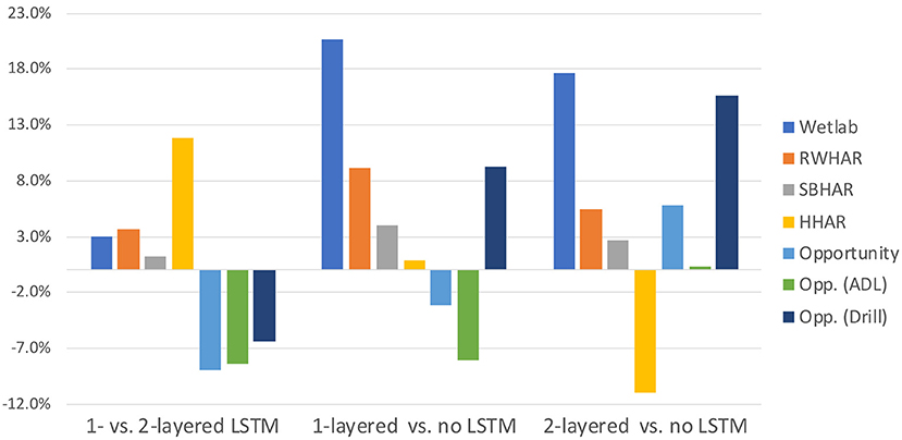
Figure 3. Average F1-score performance differences between 1-layered and 2-layered variants (1 vs. 2), 1-layered and no LSTM variants (1 vs. 0) and 2-layered and no LSTM variants (0 vs. 2) of the DeepConvLSTM architecture (Ordóñez and Roggen, 2016). A positive performance difference equates to the former outperforming the latter type of architecture. A negative performance difference equates to the latter outperforming the former type of architecture. For example a positive performance difference between 1 vs. 2 means that on average 1-layered outperformed 2-layered architectures. Contrarily a negative performance difference between 1 vs. 2 means that on average 2-layered outperformed 1-layered architectures. Reported results are averaged across 5 runs using a set of 5 varying seeds and either the Wetlab (Scholl et al., 2015), RWHAR (Sztyler and Stuckenschmidt, 2016), SBHAR (Reyes-Ortiz et al., 2016), HHAR (Stisen et al., 2015) or Opportunity dataset (Roggen et al., 2010) as input. For the Opportunity dataset results are also reported on the ADL and Drill sessions individually.
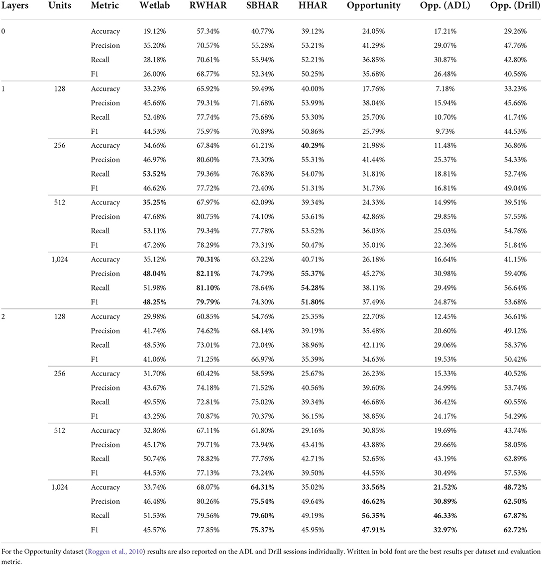
Table 1. Average cross-participant results employing a removed, 1-layered, 2-layered LSTM within the DeepConvLSTM architecture (Ordóñez and Roggen, 2016) with varying hidden units (i.e., 128, 256, 512 or 1,024) across 5 runs with a set of 5 varying seeds for the Wetlab, RWHAR, SBHAR HHAR and Opportunity dataset (Roggen et al., 2010; Scholl et al., 2015; Stisen et al., 2015; Reyes-Ortiz et al., 2016; Sztyler and Stuckenschmidt, 2016).
As previously mentioned, each dataset contains different types of activities. Analyzing results therefore on a per-class level (see Tables 2–8) reveals which type of network might be a more suited for predicting which type of activity. In their works, Ordóñez and Roggen (2016) and Hammerla et al. (2016) claim that convolutional layers are better at modeling local patterns on a sensor level, while recurrent layers are better at modeling (global) temporal patterns, e.g., of previously occurring activities. One could therefore conclude that in our experiments the convolutional network would have performed best at predicting simple/ periodical activities. Nevertheless, we could only partly exhibit this trend as the convolutional network performed best only for some simple/ periodical activities. We accredit the increased performance of the LSTM-based implementations on the simple/ periodical activities to two factors:
1. Convolutional networks are less efficient in predicting datasets with short activity execution times or rapid changes between activities.
2. All datasets were recorded following some experimental protocol which consequently introduced some form of temporal schedule amongst activities.
The first factor can particularly be seen comparing results obtained on the RWHAR (Sztyler and Stuckenschmidt, 2016), SBHAR (Reyes-Ortiz et al., 2016), and HHAR dataset (Stisen et al., 2015). Even though said datasets have an overlap in activities, i.e., sitting, standing, walking, walking_downstairs and walking_upstairs, prediction performance on these activities is significantly worse for the SBHAR dataset (Reyes-Ortiz et al., 2016). Looking at the average execution time of each activity, one can see that they are shorter within the SBHAR dataset (Reyes-Ortiz et al., 2016) compared to the other two datasets, which also causes more rapid changes between activities. At the time of writing this article, we cannot clearly identify a reason to explain this behavior. In fact, as we are using a sliding window, the duration of the activity does not influence what type of data a network sees. Nevertheless, we hypothesize that rapid changes between activities can cause more windows to consist of multiple activity labels. Given that the label of a window is determined by the label of the last sample within said window, as proposed by Ordóñez and Roggen (2016), a shorter average activity execution time can cause windows to be more likely to contain labels of multiple activites. In turn, a convolutional kernel could falsely attribute reoccurring patterns of other activities to the target activity. On the contrary, this exhibited trend could also be something specific to the SBHAR dataset (Reyes-Ortiz et al., 2016) and thus requires further investigation on a larger scale.
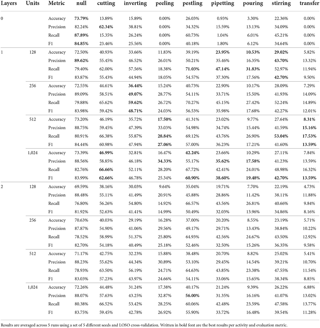
Table 2. Per class results for all 9 architectural variations of the DeepConvLSTM architecture (Ordóñez and Roggen, 2016) using the Wetlab dataset (Scholl et al., 2015) as input.

Table 3. Per class results for all 9 architectural variations of the DeepConvLSTM architecture (Ordóñez and Roggen, 2016) using the RWHAR dataset (Sztyler and Stuckenschmidt, 2016) as input.
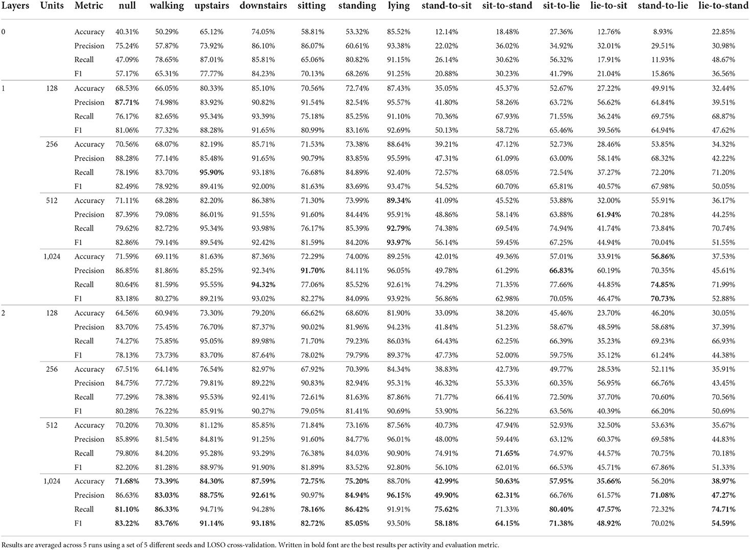
Table 4. Per class results for all 9 architectural variations of the DeepConvLSTM architecture (Ordóñez and Roggen, 2016) using the SBHAR dataset (Reyes-Ortiz et al., 2016) as input.
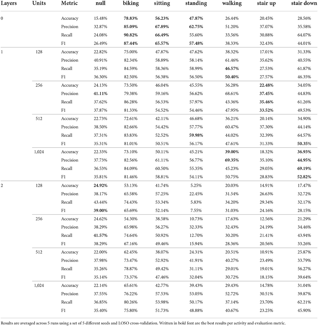
Table 5. Per class results for all 9 architectural variations of the DeepConvLSTM architecture (Ordóñez and Roggen, 2016) using the HHAR dataset (Stisen et al., 2015) as input.
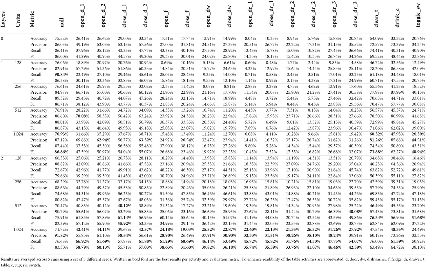
Table 6. Per class results for all 9 architectural variations of the DeepConvLSTM architecture (Ordóñez and Roggen, 2016) using the Opportunity dataset (Roggen et al., 2010) as input.
Table 7. Per class results for all 9 architectural variations of the DeepConvLSTM architecture (Ordóñez and Roggen, 2016) using the ADL sessions of the Opportunity dataset (Roggen et al., 2010) as input.
Table 8. Per class results for all 9 architectural variations of the DeepConvLSTM architecture (Ordóñez and Roggen, 2016) using the Drill sessions of the Opportunity dataset (Roggen et al., 2010) as input.
The second factor is a phenomenon which comes naturally at the cost of recording datasets in a non-natural environment or pre-scripted recording session. All datasets which were part of our analysis were recorded under experimental conditions. This involved either a predefined length of execution time, repetitions of activities or a set of steps in a predefined workflow. As already mentioned, this consequently introduces some form of temporal schedule amongst activities which can be modeled by a LSTM. Networks which include recurrent layers were thus not only able to use information on preceding activities, but also learn the overall sequence in which the activities were recorded. This type of information could especially help networks differentiate between activities which are very similar in the patterns they consist of. For example walking, walking down or walking up stairs were more reliably differentiated by networks which contained recurrent layers (see results obtained on the SBHAR, HHAR and RWHAR dataset).
Whether to employ a 1-layered or a 2-layered LSTM seems to come down to how much emphasis one wants to put on these temporal information compared to local patterns identified by the convolutional layers. This can be especially seen in the results obtained on the Drill compared to the ADL sessions of the Opportunity dataset. Former had subjects follow a strict experimental protocol with many repetitions of the same activity making temporal relations among them more strong while also introducing an overall sequence in which activities were performed. Latter had subjects not adhere to a strict experimental protocol and had them act naturally which caused temporal relationships amongst activities to be less prominent. Therefore, networks employing a 2-layered LSTM did not perform notably better than convolutional networks on the ADL sessions, while for the Drill sessions performance differences were as much as 22% in F1-score in favor of the 2-layered variants.
On the contrary, in order to correctly identify sporadic and transitional activities as seen for example in the Opportunity (Roggen et al., 2010) or SBHAR dataset (Reyes-Ortiz et al., 2016) recurrent layers seem to be necessary. We accredit this to the fact that these activities are short in time and do not show periodical, local patterns which could be identified by a convolution kernel. Moreover, similar to what Hammerla et al. (2016) concluded, transitional as well as sporadic activities like opening and closing a door, have temporal relationships with other preceding activities and can therefore be identified using the overall temporal context. We also identify this as the reason why the convolutional network is not outperforming the architectural variant with a 2-layered LSTM for the ADL sessions of the Opportunity dataset, as the dataset almost exclusively sporadic activities. Additionally, as for the simple/ periodical activities, rapid changes in activities might cause mixed sliding windows, which contain records of multiple activities. A convolutional network could thus struggle in identifying local patterns belonging to the target activity as it would more frequently see patterns belonging to other activities “incorrectly” labeled as the target activity. Nevertheless, as previously mentioned this hypothesis requires further investigation.
As previously mentioned complex activities are composed of multiple sub-activities which itself can be sporadic, transitional, or short-term periodical. In our experiments only the Wetlab dataset (Scholl et al., 2015) contains complex activities (e.g., peeling). Given that participants in the Wetlab dataset (Scholl et al., 2015) were asked to perform an experiment which required them to (mostly) follow a step-by-step guide, architectures employing recurrent layers are able to model said sequence and overall achieve better prediction results. Nevertheless, as the complex activities also inherit periodical, local patterns (e.g., stirring), employing a 1-layered LSTM seemed to combine information provided by both the recurrent and convolutional layers in the most efficient way and resulted in the highest prediction results. Nevertheless, we deem complex activities to be a case-by-case decision. Whether they are better to be predicted using a convolutional or recurrent network depends on the use case and the type of sub-activities they consist of.
With a few exceptions, performance steadily increases with an increased amount of hidden units for both the 1- and the 2-layered architectural variants. Looking at the generalization gaps within each experiment, i.e., the differences between training and validation performance, we see that generalization gaps of networks employing recurrent layers strongly correlate with the amount of increased performance one gets from recurrent layers. More specifically, this means that the larger the performance increase one gets from an LSTM, the larger the network's generalization gap will be (and vice versa). We hypothesize that this is accredited to larger LSTMs being more prone to overfit on temporal sequences in which activities were performed in the training data. Consequently, datasets who feature a strict sequence of activities, e.g., the Wetlab dataset, overfitting on such temporal patterns generally achieves better validation results than relying on local patterns in the sensor data.
In order to quantify this trend, we propose the correlation coefficient rGP. The coefficient is defined as the vectorized Pearson correlation coefficient between the generalization gap (G) and the difference in performance to the convolutional network (P) of each 1- and 2-layered architectural variant across all evaluation metrics. We report rGP for all datasets in Figure 4. Putting rGP further into context with our previous analysis, a low rGP value indicates that the learned temporal patterns are not applicable to the validation dataset. On the contrary, a high rGP value indicates the opposite, i.e., that general temporal patterns are learned. This relationship is nicely visible when dividing the Opportunity dataset into the two session types. On the one hand, when only predicting the Drill sessions rGP increases compared to its original value on the complete dataset as each subject was acting according to the same experimental protocol. On the other hand, when applied on the ADL sessions, rGP significantly decreases as the dataset does not offer prominent temporal patterns which could be learned. Our metric can thus be used as an additional indicator on the importance learned temporal patterns during the prediction process and thus how beneficial recurrent layers are to the network.
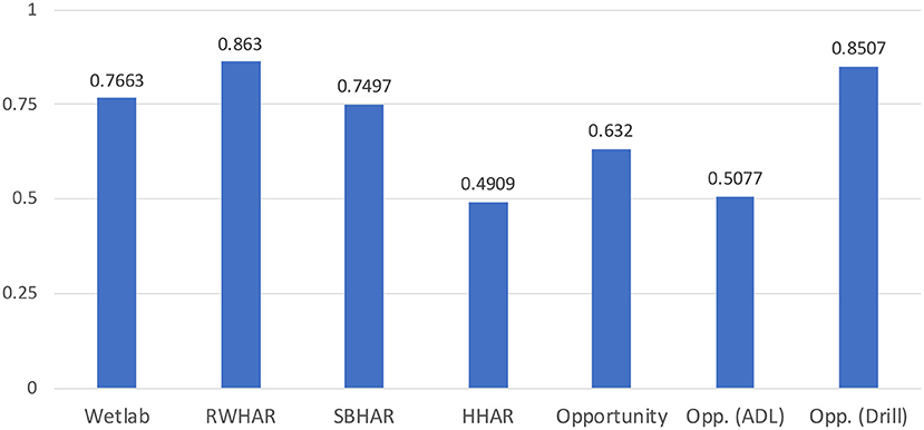
Figure 4. Calculated correlation coefficient, rGP, for each dataset. The coefficient is calculated as the vectorized Pearson correlation between the generalization gap scores (G), i.e., difference between train and validation performance, and the performance differences between the variants including recurrent layers and the convolutional network. The closer rGP is to 1, the more the network profits from including recurrent layers for the given dataset. According to rGP the RWHAR dataset (Sztyler and Stuckenschmidt, 2016) profited the most and the HHAR dataset (Stisen et al., 2015) the least from recurrent layers.
In general, our analysis suggests that larger LSTMs are more prone to overfit and rely on temporal patterns during the prediction process. Nevertheless, this can only be beneficial for datasets which contain temporal patterns and relationships among activities, and can, as seen with the HHAR dataset (Stisen et al., 2015), also lead to worse validation results.
5. Conclusion and future directions
In this article we investigated the overall necessity of recurrent layers in HAR based on results we obtained on five popular HAR datasets (Roggen et al., 2010; Scholl et al., 2015; Stisen et al., 2015; Reyes-Ortiz et al., 2016; Sztyler and Stuckenschmidt, 2016). We chose to use the DeepConvLSTM (Ordóñez and Roggen, 2016) as our architecture of choice and modified it so that it either employs 0, 1, or 2 LSTM layers. We further varied the size of the LSTM layers by employing different amounts of hidden units, i.e., 128, 256, 512, or 1,024. During analysis we tried to map characteristics of the datasets to the performance of the individual architectures, trying to identify a "rule-of-thumb" for which types of dataset and activities a convolutional network can compete with a network also including recurrent layers.
Overall, in line with what we proposed in Bock et al. (2021), employing a 1-layered LSTM delivers the best prediction results for 4 out of 5 datasets. Nevertheless, we saw large discrepancies amongst different types of activities, depending on the amount of recurrent layers. Sporadic and transitional activities, which are short in time and do not show characteristic local patterns, were most reliably predicted when using two recurrent layers. Especially the latter type of activities inherit dependencies with preceding activities and are thus more reliably predicted using the overall temporal context. Contrarily, simple/ periodical activities, which show local, reoccurring patterns, were most consistently predicted when removing the second recurrent layer. Contradicting to our expectations, architectures employing a 1-layered LSTM were more performant on simple, periodical activities than solely convolutional networks. Furthermore, we witnessed an overall trend that the performance difference between LSTM-based networks and convolutional networks grows larger for datasets which feature rapid changes and overall shorter execution times of activities.
Our results showed that bigger LSTMs are more likely to overfit and rely on learned time sequences We further noticed that the correlation between the generalization gap of a recurrent architecture and the difference in performance between the recurrent and convolutional architecture can be used to measure the effectiveness of the learned temporal patterns and thus the recurrent layers in general. Said correlation, which we defined as rGP, is high, i.e.„ close to 1, if the temporal sequences learned by the LSTM help in predicting the validation data. In contrast, said correlation is low, i.e.„ close to 0, if recurrent layers are not beneficial for the given dataset and should be omitted from the architecture. We therefore also argue that claims presented by Karpathy et al. (2015) are not applicable to sensor-based HAR, as 1-layered LSTMs were also able to learn temporal patterns. We rather argue that the depth of an effective LSTM-based RNN comes down to how much relative importance one wants to put on temporal structures compared to local structures.
To give an answer on the necessity of recurrent layers in HAR, one has to consider the type of activities and overall use case. If one mostly tries to predict sporadic and transitional activities, convolutional kernels will struggle to identify local patterns in the data. For said activities temporal context and thus recurrent layers seem to be the only effective way to reliably identify them. In general, if the goal is to train a network which predicts activities within a predefined workflow, e.g., an experiment or production process, recurrent layers are beneficial and should be included in the final architecture. More specifically our experiments showed that a 1-layered LSTM deemed to be most effective in predicting activities within a predefined workflow, suggesting that it most efficiently combines both temporal and local information and is less prone to overfitting solely on the former. On the contrary, our results also suggest that in order to train a general system which predicts simple/ periodical activities, one should not include recurrent layers as they increase the risk of relying too much on temporal patterns which will not be present in the real-world application scenario. Unlike complex activities, simple/ periodical activities do not consist of in-activity sequences. Therefore, having the 1-layered variants outperform architectures employing no LSTM layer, suggests that said performance increase might be due to temporal dependencies amongst activities which were introduced during recording of the datasets. Given that a network is more likely to overfit on temporal patterns when employing two LSTM layers and that datasets like the RWHAR dataset (Sztyler and Stuckenschmidt, 2016) do not intend to model a certain activity workflow, having a 1-layered LSTM still produce the best prediction results along with a rGP coefficient close to 1, makes us assume that models indeed learned (unwanted) temporal patterns. We also saw that for datasets which featured rapid changes between activities, convolutional networks were not as performant as recurrent networks in predicting simple/ periodical activities, causes us to think that latter networks took advantage of temporal patterns within said datasets.
Generally speaking, even though results we obtained during our experiments on paper suggest that LSTMs should be included at all times, we argue that, depending on the underlying use case, high benchmark scores on currently available HAR datasets can give a false sense of security and do not automatically ensure overall generability of trained models. We notice that for datasets which do not try to model a temporal process, e.g., the RWHAR dataset (Sztyler and Stuckenschmidt, 2016), including recurrent layers made networks learn the overall order in which activities were recorded, which, though increasing the benchmark score, would not benefit a model in a real-world setting and could even end up hurting the predictive performance as the model would rely on unnatural temporal patterns. Furthermore, we witnessed a significant decrease in performance for convolutional networks once simple/ periodical activities are changing more rapidly along with the fact that sporadic activities were not at all reliably detected using convolutional kernels. As in said cases temporal context deemed necessary, one has to question whether they would be able to be detected if naturally said context does not exist, but either only exists because of existing “partner”-relations among activities (e.g.„ opening and closing a cupboard), preceding activities (e.g., a person was sitting, thus sit-to-stand is very likely) or an experimental protocol. To conclude, the metric we introduced in this article, rGP, be used to measure the effectiveness and applicability of learned temporal patterns and thus also be used as a decision metric whether to employ recurrent layers within the network.
To further examine the applicability of the introduced metric rGP, our next steps within this research are four-fold. First, in order to prove that networks featuring recurrent layers are prone to overfitting on unwanted temporal patterns, we will explore regularization techniques which omit said temporal patterns and only keep those which can be expected to be witnessed in a real-world setting. Especially the RWHAR dataset offers a basis for such an analysis as it intends to model “independent” activities. We expect that putting such regularization techniques in place will end up hurting the performance of the networks which include recurrent layers, while leaving convolutional networks mostly unaffected. Second, we will further investigate the reason for why convolutional networks are less performant, especially for simple/ periodical activities, for datasets which contain rapid changes and thus short average execution times of activities. We already hypothesized that due to the nature how we define sliding windows, i.e., by the label of the last sample, a dataset which features rapid changes thus also contains more likely “mixed” windows, i.e., ones which contain multiple labels. In order to explore whether this is true, we plan to modify datasets to omit said “mixed” windows and see whether a convolutional network is more performant when only being trained on windows which only contain local patterns of the window label. Thirdly, we plan to expand our choice of datasets included in our analysis. We like to include datasets which (1) have subjects perform simple/ periodical activities without any restrictions or underlying protocol, (2) consist of data obtained from a larger number of participants than our current choice of datasets and (3) include complex activities. Lastly, we plan to apply similar architectural changes to recurrent parts of other popular HAR networks, for example Abedin et al. (2021) or Dirgová Luptáková et al. (2022).
Data availability statement
Solely publicly available datasets were analyzed in this study. The code used for conducting experiments, links to the datasets as well as log files of all experiments can be found at: https://github.com/mariusbock/recurrent_state_of_the_art.
Author contributions
MB conducted the experiments and wrote the manuscript. AH performed the analysis of each dataset along with the color-coded visualization of the sensor data. AH, KV, and MM also contributed to the writing. All authors contributed equally in the analysis of the results.
Funding
This work received support from the House of Young Talents at the University of Siegen.
Conflict of interest
The authors declare that the research was conducted in the absence of any commercial or financial relationships that could be construed as a potential conflict of interest.
Publisher's note
All claims expressed in this article are solely those of the authors and do not necessarily represent those of their affiliated organizations, or those of the publisher, the editors and the reviewers. Any product that may be evaluated in this article, or claim that may be made by its manufacturer, is not guaranteed or endorsed by the publisher.
Footnotes
References
Abedin, A., Ehsanpour, M., Shi, Q., Rezatofighi, H., and Ranasinghe, D. C. (2021). “Attend and discriminate: beyond the state-of-the-art for human activity recognition using wearable sensors,” in Proceedings of the ACM on Interactive, Mobile, Wearable and Ubiquitous Technologies, Vol. 5 (New York, NY).
Bachlin, M., Roggen, D., Troster, G., Plotnik, M., Inbar, N., Meidan, I., et al. (2009). “Potentials of enhanced context awareness in wearable assistants for Parkinson's disease patients with the freezing of gait syndrome,” in International Symposium on Wearable Computers (Linz), 123–130.
Bock, M., Hölzemann, A., Moeller, M., and Van Laerhoven, K. (2021). “Improving deep learning for HAR with shallow LSTMs,” in International Symposium on Wearable Computers (New York, NY), 7–12.
Bordes, A., Chopra, S., and Weston, J. (2014). “Question answering with subgraph embeddings,” in Proceedings of the 2014 Conference on Empirical Methods in Natural Language Processing (Doha), 615–620.
Chen, K., Zhang, D., Yao, L., Guo, B., Yu, Z., and Liu, Y. (2021). Deep learning for sensor-based human activity recognition: overview, challenges, and opportunities. ACM Comput. Surveys 54, 1–40. doi: 10.1145/3447744
Collobert, R., Weston, J., Bottou, L., Karlen, M., Kavukcuoglu, K., and Kuksa, P. (2011). Natural language processing (Almost) from scratch. J. Mach. Learn. Res. 12, 2493–2537. Available online at: http://jmlr.org/papers/v12/collobert11a.html
Dirgová Luptákov,á, I., Kubovčík, M., and Pospíchal, J. (2022). Wearable Sensor-Based Human Activity Recognition With Transformer Model. Sensors 22. doi: 10.3390/s22051911
Dua, N., Singh, S. N., and Semwal, V. B. (2021). Multi-input CNN-GRU based human activity recognition using wearable sensors. Computing 103, 1461–1478. doi: 10.1007/s00607-021-00928-8
Edel, M., and Köppe, E. (2016). “Binarized-BLSTM-RNN based human activity recognition,” in International Conference on Indoor Positioning and Indoor Navigation (Alcala de Henares), 1–7.
Farabet, C., Couprie, C., Najman, L., and LeCun, Y. (2013). Learning hierarchical features for scene labeling. IEEE Trans. Pattern. Anal. Mach. Intell. 35, 1915–1929. doi: 10.1109/TPAMI.2012.231
Glorot, X., and Bengio, Y. (2010). “Understanding the difficulty of training deep feedforward neural networks,” in Proceedings of the 13th International Conference on Artificial Intelligence and Statistics, volume 9 of Proceedings of Machine Learning Research, eds Y. W. The and M. Titterington (Sardinia), 249–256.
Guan, Y., and Plötz, T. (2017). “Ensembles of deep LSTM learners for activity recognition using wearables,” in Proceedings of the ACM on Interactive, Mobile, Wearable and Ubiquitous Technologies, Vol. 1 (New York, NY).
Hammerla, N. Y., Halloran, S., and Ploetz, T. (2016). “Deep, convolutional, and recurrent models for human activity recognition using wearables,” in Proceedings of the 25th International Joint Conference on Artificial Intelligence (New York, NY), 1533–1540.
Haresamudram, H., Beedu, A., Agrawal, V., Grady, P. L., Essa, I., Hoffman, J., et al. (2020). “Masked reconstruction based self-supervision for human activity recognition,” in Proceedings of the International Symposium on Wearable Computers (New York, NY), 45–49.
Hinton, G., Deng, L., Yu, D., Dahl, G. E., Mohamed, A.-,r., Jaitly, N., et al. (2012). Deep neural networks for acoustic modeling in speech recognition: the shared views of four research groups. IEEE Signal Process. Mag. 29, 82–97. doi: 10.1109/MSP.2012.2205597
Inoue, M., Inoue, S., and Nishida, T. (2018). Deep recurrent neural network for mobile human activity recognition with high throughput. Artif. Life Rob. 23, 173–185. doi: 10.1007/s10015-017-0422-x
Jaakkola, T., and Haussler, D. (1998). “Exploiting generative models in discriminative classifiers,” in Advances in Neural Information Processing Systems, Vol. 11 (Denver, CO).
Jean, S., Cho, K., Memisevic, R., and Bengio, Y. (2014). “On using very large target vocabulary for neural machine translation,” in Proceedings of the 53rd Annual Meeting of the Association for Computational Linguistics and the 7th International Joint Conference on Natural Language Processing (Volume 1: Long Papers) (Beijing), 1–10.
Karpathy, A., Johnson, J., and Li, F.-F. (2015). Visualizing and understanding recurrent networks. CoRR, abs/1506.02078.
Krizhevsky, A., Sutskever, I., and Hinton, G. E. (2012). “ImageNet classification with deep convolutional neural networks,” in Proceedings of the 25th International Conference on Neural Information Processing Systems, Vol. 1 (Lake Tahoe, NV), 1097–1105.
Lester, J., Choudhury, T., and Borriello, G. (2006). “A practical approach to recognizing physical activities,” in International Conference on Pervasive Computing (Dublin), 1–16.
Lester, J., Choudhury, T., Kern, N., Borriello, G., and Hannaford, B. (2005). “A hybrid discriminative/generative approach for modeling human activities,” in 19th International Joint Conference on Artificial Intelligence (Edinburgh), 766–772.
Liao, L., Fox, D., and Kautz, H. (2005). “Location-based activity recognition using relational markov networks,” in 19th International Joint Conference on Artificial Intelligence, Vol. 5 (Edinburgh), 773–778.
Mikolov, T., Deoras, A., Povey, D., Burget, L., and Černocký, J. (2011). “Strategies for training large scale neural network language models,” in IEEE Workshop on Automatic Speech Recognition &Understanding (Waikoloa, HI: IEEE), 196–201.
Murahari, V. S., and Plötz, T. (2018). “On attention models for human activity recognition,” in Proceedings of the 2018 ACM International Symposium on Wearable Computers, ISWC '18 (Singapore), 100–103.
Najafabadi, M. M., Villanustre, F., Khoshgoftaar, T. M., Seliya, N., Wald, R., and Muharemagic, E. (2015). Deep learning applications and challenges in big data analytics. J. Big Data 2, 1. doi: 10.1186/s40537-014-0007-7
Ordóñez, F. J., and Roggen, D. (2016). Deep convolutional and LSTM recurrent neural networks for multimodal wearable activity recognition. Sensors 16, 115. doi: 10.3390/s16010115
Patterson, D. J., Fox, D., Kautz, H., and Philipose, M. (2005). “Fine-grained activity recognition by aggregating abstract object usage,” in 9th International Symposium on Wearable Computers (Osaka), 44–51.
Pouyanfar, S., Sadiq, S., Yan, Y., Tian, H., Tao, Y., Reyes, M. P., et al. (2018). A survey on deep learning: algorithms, techniques, and applications. ACM Comput. Surveys 51, 1–36. doi: 10.1145/3234150
Reddy, S., Mun, M., Burke, J., Estrin, D., Hansen, M., and Srivastava, M. (2010). Using mobile phones to determine transportation modes. Trans. Sensor Networks 6, 1–27. doi: 10.1145/1689239.1689243
Reiss, A., and Stricker, D. (2012). “Introducing a new benchmarked dataset for activity monitoring,” in 2012 16th International Symposium on Wearable Computers (Newcastle: IEEE).
Reyes-Ortiz, J.-L., Oneto, L., Sam,à, A., Parra, X., and Anguita, D. (2016). Transition-aware human activity recognition using smartphoneson-body localization of wearable devices: an investigation of position-aware activity recognition. Neurocomputing 171, 754–767. doi: 10.1016/j.neucom.2015.07.085
Roggen, D., Calatroni, A., Rossi, M., Holleczek, T., Förster, K., Tröster, G., et al. (2010). “Collecting complex activity datasets in highly rich networked sensor environments,” in 7th International Conference on Networked Sensing Systems (Kassel: IEEE), 233–240.
Sainath, T. N., Mohamed, A.-R., Kingsbury, B., and Ramabhadran, B. (2013). “Deep convolutional neural networks for LVCSR,” in IEEE International Conference on Acoustics, Speech and Signal Processing (Vancouver, BC), 8614–8618.
Scholl, P. M., Wille, M., and Van Laerhoven, K. (2015). “Wearables in the wet lab: a laboratory system for capturing and guiding experiments,” in UbiComp '15: Proceedings of the 2015 ACM International Joint Conference on Pervasive and Ubiquitous Computing (Osaka), 589–599.
Stisen, A., Blunck, H., Bhattacharya, S., Prentow, T. S., Kjærgaard, M. B., Dey, A., et al. (2015). “Smart devices are different: assessing and mitigatingmobile sensing heterogeneities for activity recognition,” in 13th Conference on Embedded Networked Sensor Systems (Seoul: ACM), 127–140.
Sutskever, I., Vinyals, O., and Le, Q. V. (2014). “Sequence to sequence learning with neural networks,” in Proceedings of the 27th International Conference on Neural Information Processing Systems, Vol. 2 (Montreal, QC), 3104–3112.
Szegedy, C., Liu, W., Jia, Y., Sermanet, P., Reed, S. E., Anguelov, D., et al. (2015). “Going deeper with convolutions,” in Proceedings of the IEEE Conference on Computer Vision and Pattern Recognition, CVPR (Boston, MA: IEEE).
Sztyler, T., and Stuckenschmidt, H. (2016). “On-Body localization of wearable devices: an investigation of position-aware activity recognition,” in International Conference on Pervasive Computing and Communications (Sydney, NSW: IEEE), 1–9.
Tompson, J., Jain, A., LeCun, Y., and Bregler, C. (2014). “Joint training of a convolutional network and a graphical model for human pose estimation,” in Proceedings of the 27th International Conference on Neural Information Processing Systems (Montreal, QC), 1799–1807.
van Kasteren, T., Noulas, A., Englebienne, G., and Kröse, B. (2008). “Accurate activity recognition in a home setting,” in 10th International Conference on Ubiquitous Computing (Seoul), 1–9.
Xi, R., Hou, M., Fu, M., Qu, H., and Liu, D. (2018). “Deep dilated convolution on multimodality time series for human activity recognition,” in International Joint Conference on Neural Networks (Rio de Janeiro), 1–8.
Xu, C., Chai, D., He, J., Zhang, X., and Duan, S. (2019). InnoHAR: a deep neural network for complex human activity recognition. IEEE Access 7, 9893–9902. doi: 10.1109/ACCESS.2018.2890675
Yuki, Y., Nozaki, J., Hiroi, K., Kaji, K., and Kawaguchi, N. (2018). “Activity recognition using dual-ConvLSTM extracting local and global features for SHL recognition challenge,” in International Joint Conference and International Symposium on Pervasive and Ubiquitous Computing and Wearable Computers (Singapore), 1643–1651.
Keywords: human activity recognition, CNN-RNNs, deep learning, network architectures, datasets
Citation: Bock M, Hoelzemann A, Moeller M and Van Laerhoven K (2022) Investigating (re)current state-of-the-art in human activity recognition datasets. Front. Comput. Sci. 4:924954. doi: 10.3389/fcomp.2022.924954
Received: 20 April 2022; Accepted: 01 September 2022;
Published: 30 September 2022.
Edited by:
Katia Vega, University of California, Davis, United StatesCopyright © 2022 Bock, Hoelzemann, Moeller and Van Laerhoven. This is an open-access article distributed under the terms of the Creative Commons Attribution License (CC BY). The use, distribution or reproduction in other forums is permitted, provided the original author(s) and the copyright owner(s) are credited and that the original publication in this journal is cited, in accordance with accepted academic practice. No use, distribution or reproduction is permitted which does not comply with these terms.
*Correspondence: Marius Bock, marius.bock@uni-siegen.de