Best Practices for Elevation-Based Assessments of Sea-Level Rise and Coastal Flooding Exposure
 Dean B. Gesch
- U.S. Geological Survey, Earth Resources Observation and Science Center, Sioux Falls, SD, United States
Elevation data are critical for assessments of sea-level rise (SLR) and coastal flooding exposure. Previous research has demonstrated that the quality of data used in elevation-based assessments must be well understood and applied to properly model potential impacts. The cumulative vertical uncertainty of the input elevation data substantially controls the minimum increments of SLR and the minimum planning horizons that can be effectively used in assessments. For regional, continental, or global assessments, several digital elevation models (DEMs) are available for the required topographic information to project potential impacts of increased coastal water levels, whether a simple inundation model is used or a more complex process-based or probabilistic model is employed. When properly characterized, the vertical accuracy of the DEM can be used to report assessment results with the uncertainty stated in terms of a specific confidence level or likelihood category. An accuracy evaluation has been conducted of global DEMs to quantify their inherent vertical uncertainty to demonstrate how accuracy information should be considered when planning and implementing a SLR or coastal flooding assessment. The evaluation approach includes comparison of the DEMs with high-accuracy geodetic control points as the independent reference data over a variety of coastal relief settings. The global DEMs evaluated include SRTM, ASTER GDEM, ALOS World 3D, TanDEM-X, NASADEM, and MERIT. High-resolution, high-accuracy DEM sources, such as airborne lidar and stereo imagery, are also included to give context to the results from the global DEMs. The accuracy characterization results show that current global DEMs are not adequate for high confidence mapping of exposure to fine increments (<1 m) of SLR or with shorter planning horizons (<100 years) and thus they should not be used for such mapping, but they are suitable for general delineation of low elevation coastal zones. In addition to the best practice of rigorous accounting for vertical uncertainty, other recommended procedures are presented for delineation of different types of impact areas (marine and groundwater inundation) and use of regional relative SLR scenarios. The requirement remains for a freely available, high-accuracy, high-resolution global elevation model that supports quantitative SLR and coastal inundation assessments at high confidence levels.
Introduction
The effects of sea-level rise (SLR) and other sources of increased water levels along the world’s coastlines are pervasive and varied (Williams, 2013). Because of the low-lying nature of many coastal lands, the topography, or elevation in relation to sea level, largely controls their exposure to adverse effects of increased water levels, both chronic conditions (SLR) and episodic events (storm surge inundation or king tide flooding). Elevation data, often in the form of digital elevation models (DEMs), are therefore critical for assessments of exposure, and corresponding vulnerability and risk, to permanent or temporary flooding and other effects of increased water levels along the coast.
For nearly four decades, elevation data, most often in the form of DEMs, have been used to identify low-lying coastal lands over broad areas to conduct assessments of the effects of rising sea levels (Schneider and Chen, 1980; Titus et al., 1991; Titus and Richman, 2001; Small and Nicholls, 2003; Ericson et al., 2006; Rowley et al., 2007; Dasgupta et al., 2008, 2010; Weiss et al., 2011; Haer et al., 2013; Blankespoor et al., 2014; Neumann et al., 2015; Hardy and Nuse, 2016; Kulp and Strauss, 2017; Small et al., 2018; Wolff et al., 2018). Over this period, the quality of DEMs available for use in assessments has improved, especially in terms of spatial resolution and vertical accuracy. For large-area assessments (regional, continental, global), several choices are available for DEMs for the required topographic information to project potential impacts of increased coastal water levels, whether a simple inundation model is used or a more complex process-based or probabilistic model is employed. Previous research has demonstrated that the quality of data, and associated transformations, used for elevation-based assessments must be well understood and applied to properly model potential impacts (Gesch, 2009; Coveney and Fotheringham, 2011; Cooper and Chen, 2013; Cooper et al., 2013, 2015; Gesch, 2013; Schmid et al., 2014; Dahl et al., 2017; Jones et al., 2017; West et al., 2018).
Uncertainty in climate change and coastal hazard assessments has been addressed in numerous studies. Le Cozannet et al. (2015, 2017) and Stephens et al. (2017) discuss the importance of considering uncertainties from all sources in assessments of sea-level change, but they do not specifically mention vertical uncertainty of topographic data used to map potential impact zones on the land surface. A number of studies address the effects of input elevation data uncertainty (Gesch, 2009; Kettle, 2012; Bell et al., 2014; Hinkel et al., 2014; Valentine, 2014) and conclude that higher resolution data with better vertical accuracy significantly improve assessment results. The choice of elevation model for an assessment study can also have a substantial effect on results owing to combined uncertainties of input datasets, especially elevation and population distribution (Lichter et al., 2011; Mondal and Tatem, 2012; Wolff et al., 2016). The result of many SLR assessments is a set of maps that spatially show the areas exposed to inundation or other adverse effects of specific scenarios of sea-level change, and such maps are enhanced by including a description of mapping uncertainty (Kostelnick et al., 2013; Retchless, 2018), often expressed as a confidence level.
Recently, within the coastal hazard modeling community there has been continued recognition that vertical uncertainty should be accounted for quantitatively to improve impact mapping and assessment. National Oceanic and Atmospheric Administration [NOAA] (2010) and Doyle et al. (2015) recognize that DEM vertical accuracy is a critical element in SLR impact assessments and that the uncertainties contributed by elevation data and its associated transformations should be explicitly addressed. Fortunately, there is a rich heritage of technical work on assessing vertical uncertainty (DEM error), its consequences and implications, and its use in improving applications (Hunter and Goodchild, 1995; Fisher and Tate, 2006; Wechsler and Kroll, 2006; Maune et al., 2007; Wechsler, 2007; Höhle and Höhle, 2009), and this body of work can be relied upon as a basis for approaches to rigorous handling of uncertainty in coastal inundation assessments.
The importance of the quality (spatial resolution and vertical accuracy) of the input elevation information in inundation assessments has been well recognized in some studies (Bales and Wagner, 2009; Coveney and Fotheringham, 2011; Zhang, 2011; Fraile-Jurado and Ojeda-Zújar, 2012; Sampson et al., 2016; Wolff et al., 2016; Mogensen and Rogers, 2018; Paprotny et al., 2018; Vousdoukas et al., 2018); however, numerous other studies make no mention of the uncertainty of the critical input elevation layer and the implications for the reliability of the results. There is a variety of DEMs with global or near global coverage mostly derived from remote sensing (Gesch, 2012b; Sampson et al., 2016) available for use in inundation modeling and assessment, yet better data are needed (Simpson et al., 2015). Therefore, it is critical that producers of such assessments understand, characterize, and describe the cumulative uncertainties from the underlying elevation data and associated transformations that propagate to the assessment results (maps and estimates of impacted area and resources). The purpose of this paper is to document the best practices in properly accounting for the vertical uncertainty inherent in all elevation-based SLR and coastal flooding assessments. Additionally, other best practices for such assessments extracted from the scientific record of successful studies are listed and described. Establishment of best practices, or standardized methodology, is recognized as an important advance in improving the usefulness of climate change vulnerability mapping at various scales and for multiple classes of stakeholders and end users (Preston et al., 2011).
Materials and Methods
When an elevation-based SLR or coastal flooding assessment is conducted, especially over broad areas, a simple inundation method known as the “bathtub” model is often used, an approach that has also been referred to as the “single-value surface” (National Oceanic and Atmospheric Administration [NOAA], 2010), “equilibrium” (Gallien et al., 2011), “planar” (Bates and De Roo, 2000), “hydrostatic” (Habel et al., 2017), and “static inundation” (Paprotny et al., 2018) method. To delineate the inundation zone with the bathtub method, the water level is simply raised on a coastal DEM by selecting all areas that are below the specified new water level height. The approach is improved by enforcing hydrologic connectivity (Poulter and Halpin, 2007; Poulter et al., 2008), ensuring that flooded areas have a direct hydrologic connection to the ocean, which is recommended as a best practice for coastal assessments. Limitations of the bathtub modeling approach have been identified (Passeri et al., 2015; Boyd et al., 2016), including failure of the DEM to represent the detailed hydraulic connections and barriers needed for accurate spatially explicit flood mapping (Gallien et al., 2011, 2013). Bathtub modeling can overpredict flood extent compared to hydraulic and hydrodynamic modeling approaches (Gallien et al., 2011, 2014; Seenath et al., 2016), especially at local scales, yet the simple approach realizes savings in input data and computation requirements (Kovanen et al., 2018) and under certain conditions can perform nearly as well as more complex models (Bates and De Roo, 2000). Another important consideration in using simple inundation models to assess potential impacts of raised coastal water levels is to recognize that not all areas will respond to increased water levels by simply becoming inundated (Gesch et al., 2009; Passeri et al., 2015; Lentz et al., 2016). Instead, some areas will adapt by responding dynamically. In these cases, maps of potential impact zones derived from simple bathtub models will indicate areas that may be affected by sea-level change, but not necessarily transition to permanent open water.
Notwithstanding the known limitations of bathtub modeling, the approach remains widely employed for coastal impact assessments, likely due to its ease of application, especially for initial screening and inventory across large areas. Thus, the analysis and discussion below on properly accounting for vertical uncertainty is directly relevant to simple inundation modeling. However, it is also applicable to more complex physical process-based and probabilistic models because they too invariably need to measure increased water levels, and elevation data are required to do so; therefore, vertical uncertainty must be considered.
Accounting for Uncertainty in Exposure Assessments
The importance of considering uncertainty in general in climate change assessments, and more specifically vertical uncertainty in SLR and coastal flooding studies of interest here, is well established in the previously cited literature. There is a long record of research on uncertainty in geospatial data, with much of it focused on DEMs and other forms of elevation data (Hunter and Goodchild, 1995; Fisher, 1998; Fisher and Tate, 2006; Wechsler and Kroll, 2006; Wechsler, 2007; Höhle and Höhle, 2009). The approaches to handling vertical uncertainty can be categorized into three methods: (1) ignore it; (2) apply a global error estimate; (3) model the error distribution and then perform spatial error propagation through simulation. Each of these categories is described more fully below. Hunter and Goodchild (1995) use the same construct of three general approaches, and they illustrate by use of an elevation contour example.
Most elevation-based SLR assessments mention the DEM used, but many stop there and ignore the inherent vertical uncertainty or the common description of such, the vertical accuracy (or error). The user of such an assessment is left to guess about the quality of the results, and in the case of a user with little familiarity with elevation data, the implications of vertical error are completely unrepresented and thus cannot be factored into decision making. Some studies at least mention the vertical error in the underlying elevation data, and perhaps generally discuss its implications, but make no attempt to quantify spatially how the uncertainty reflected in that vertical error affects the results (Mcleod et al., 2010; Emrich and Cutter, 2011; Kuhn et al., 2011; Weiss et al., 2011; Haer et al., 2013, 2018; Maloney and Preston, 2014). The assessments that fall into this first category do not explicitly consider uncertainty, and they are labeled as “deterministic” as the delineation of the impact zone has no indication of the quality of that mapping, nor is there any expression of confidence that is associated with the results. The location and extent of the inundation zone is determined simply by where the chosen elevation of the raised water level falls on the landscape.
The second category of approaches to handling vertical uncertainty includes assessments that apply a global error metric, such as the widely used root mean square error (RMSE) or a related measure such as “linear error at 95% confidence” (LE95) (Maune et al., 2007). This method equally applies the full global error estimate everywhere, which assumes that all areas are subject to the full range of vertical error. Thus, this approach can be thought of as a worst-case scenario, and the results reflect a range incorporating the minimum and maximum extremes of error. In practice, the full error is applied both above and below a specified elevation (usually representing a raised water level) by adding and subtracting it to the elevation, respectively, and then using those two new elevations in bathtub modeling to delineate the maximum and minimum impact zones (Gesch, 2013). In essence, each delineation is still a deterministic mapping, thus this approach is called here the “modified deterministic” method. It has the advantage over the straight deterministic method in that it addresses uncertainty by bounding the error range and assigning a label of quantified confidence based on the portion of the full error probability distribution represented by the error metric applied, for instance 68% confidence in the case of RMSE or 95% confidence in the case of LE95 (for an unbiased normal distribution of errors). For users of such assessment results, the stated confidence level indicates how confident the user can be that the true extent of the impact zone is contained within the given range (between the minimum and maximum areas). Examples of the successful use of the modified deterministic approach are found in Gilmer and Ferdaña (2012), Gesch (2013), Nielsen and Dudley (2013), and Enwright et al. (2015).
The third category of approaches to accounting for vertical uncertainty includes methods that model the elevation error distribution and then propagate that error spatially through Monte Carlo simulation (Temme et al., 2009). The result of such an operation is a map containing the spatial distribution of the probable errors, which can be used to indicate the likelihood, or probability, of any location falling above or below a specified elevation, thus this approach is called the “probabilistic” method. There is a long history of treating elevation error probabilistically (Hunter and Goodchild, 1995; Fisher, 1998; Zerger et al., 2002; Wechsler and Kroll, 2006), and the approach has been applied successfully in several recent SLR and flooding assessments (Cooper and Chen, 2013; Leon et al., 2014; Cooper et al., 2015; Enwright et al., 2017; Fereshtehpour and Karamouz, 2018). In using the probabilistic approach, random error fields that match the error distribution characteristics derived from DEM accuracy assessment are generated and applied spatially. The assumption is that the elevation error is random, but elevation exhibits spatial autocorrelation, thus the error also has spatial autocorrelation (Wechsler and Kroll, 2006). Two techniques have been used to account for spatially autocorrelated errors in propagation through simulation: increasing the spatial autocorrelation in the random error fields by spatial filtering before they are applied to the DEM (Torio and Chmura, 2013; Enwright et al., 2017), and error modeling through sequential Gaussian simulation (Leon et al., 2014; Fereshtehpour and Karamouz, 2018). Other implementations of the probabilistic approach to handling vertical uncertainty in SLR assessments do not explicitly account for spatially autocorrelated elevation error (Cooper and Chen, 2013; Cooper et al., 2015; West et al., 2018), so they could be thought of as a type of worst-case scenario where the error is completely random without any spatial dependence on elevation. For users of assessments following the probabilistic approach, the stated probability indicates the likelihood, or chance, that the delineated area will be impacted or flooded at the specified water level, for example a 95% chance (or at least 95 times out of 100) that the area will be inundated.
The modified deterministic and probabilistic methods of accounting for vertical uncertainty are preferred as best practices over the simple deterministic method that ignores the effects of elevation error. With the preferred modified deterministic and probabilistic methods, maps of impact areas, and the associated inventory of population and resources located within impact zones, have increased value because of attached statements of confidence level or probability. The probabilistic approach is an excellent choice for a study that has ready access to sufficient compute resources required for error propagation through simulation, especially if the study area is large and the input data have high spatial resolution. Alternatively, the modified deterministic approach is suitable and is recommended. The results of the probabilistic method allow selection of different probabilities with which to present maps or statistics of areas exposed to inundation, while the modified deterministic method is less flexible in that it presents results within a bounded range at a specific confidence level. For the probabilistic method, if the full reference dataset used for accuracy assessment of the DEM is available, then a measure of spatial autocorrelation of the errors can be made and subsequent sequential Gaussian simulation can be performed. However, if only a global measure of the DEM vertical accuracy is available, for instance RMSE, then a good choice is to perform spatial filtering of the random error fields to account for autocorrelation as part of the simulation process for error propagation.
In recognition of the importance of considering vertical uncertainty in assessments of SLR and flooding exposure, there is a critical choice of parameters that must be made at the outset of a study: the increment of water level increase to be modeled, and the planning horizon (timeframe of projection into the future). The next three subsections (Minimum Sea-Level Rise Increment, Cumulative Vertical Uncertainty, and Minimum Planning Timeline) describe how the selection of these parameters needs to consider the vertical quality of the input elevation data (and associated datum transformations) and how the choices affect the reliability, or confidence level, of the assessment results.
Minimum Sea-Level Rise Increment
Any elevation-based SLR or coastal flooding assessment that uses a DEM, whether a simple bathtub model or a more complex hydraulic model is employed, raises the water level on a geospatial dataset that represents the topography of the study area. Such a process is essentially an elevation contouring process whereby a line of constant elevation (at the selected water level increase) is derived from the spatial arrangement of individual elevation values at discrete locations (usually in a regular grid in the case of a raster DEM). It is easy to define such an elevation contour, especially in a digital geographic information system (GIS), and the vertical increment between adjacent contours, referred to as the contour interval, is a parameter that must be specified in the procedure. A small interval can be applied to any DEM, but doing so does not imply that the derived contours automatically meet published accuracy standards. The interval must not be so small that it falls within the bounds of vertical error of the DEM, as such an operation would place the measurement (elevation increment) “in the noise” of the underlying elevation data. In the case of SLR or flooding assessments, the amount of water level increase from its current elevation to a future projected elevation is analogous to the contour interval, and that increment of increase must be larger than the inherent vertical error of the DEM for the projected future level to have a high level of confidence.
Based on the concept of elevation contour line accuracy, a method has been developed (Gesch, 2012a, 2013) to determine the minimum contour interval, or in the present case, the minimum increment of water level increase that can be used to meet a specified confidence level. Using the minimum increment in an assessment ensures that the chosen study parameter (amount of SLR or flooding level) is truly supported by the DEM and is not too small given the inherent vertical uncertainty. In the U.S., legacy national map accuracy standards applied to topographic contour maps specify that 90% of tested elevations should fall within one-half of the map contour interval (Maune et al., 2007), and this has been called the vertical map accuracy standard (VMAS) with a 90% confidence level, or alternatively “linear error at 90% confidence” (LE90). From the map user perspective, elevations determined from the map on 9 out of 10 points will have true elevations that are within one-half of the contour interval (CI). The contour accuracy standard is expressed in the following equation:
Rearranging this simple equation as
allows the contour interval to be expressed as a factor of the elevation data accuracy. Additional accuracy standards developed more recently for digital geospatial data rather than hardcopy maps, such as the National Standard for Spatial Data Accuracy (Maune et al., 2007) and the American Society for Photogrammetry and Remote Sensing (ASPRS) Positional Accuracy Standards for Digital Geospatial Data (ASPRS, 2015), provide procedures for direct conversion among DEM accuracy metrics and equivalent contour intervals. For instance, much of the coastal and floodplain light detection and ranging (lidar) data in the U.S. was collected to a product specification by the Federal Emergency Management Agency (FEMA) for DEMs with an RMSE of 0.185 m, which was calculated to provide elevation data that would support topographic mapping at a 2-foot (0.61 m) contour interval accuracy (Maune et al., 2007).
In the present case of SLR or coastal flooding, the increment of water level increase is analogous to the contour interval because raising the water level on an elevation dataset is equivalent to a contouring operation, especially when multiple successive water levels are mapped. Thus, the minimum water level increment for modeling can be stated directly as a factor of the elevation data accuracy, expressed as a common vertical error metric (LE90 in the preceding example). Two of the most commonly used DEM error metrics are RMSE and LE95, and direct translations among RMSE, LE90, and LE95 are available (Maune et al., 2007), assuming the errors are from an unbiased normal distribution. Because the error metrics represent a portion of the cumulative probability distribution of errors, a confidence level can be stated for the minimum increment, for example 68% confidence for RMSE (equivalent to the “one sigma” error, or standard deviation of the errors for an unbiased normal distribution), 90% confidence for LE90, and 95% confidence for LE95. Zhang et al. (2011) recognize that the modeled increments of SLR should be tied to the inherent vertical error, and they did so by selecting increments that matched the RMSE of their input DEM, whereas the approach described here has the added advantage of providing a direct method to calculate the proper increments as a function of the DEM accuracy at a specific confidence level. This approach, rooted in contour interval accuracy standards, provides the quantitative basis for the “guideline” (Gesch et al., 2009) and “rule of thumb” (National Oceanic and Atmospheric Administration [NOAA], 2010) that the increment of SLR modeled should be at least twice the vertical accuracy of the elevation data.
As an example to illustrate, consider a DEM with an RMSE of 0.15 m derived from airborne lidar data. Assuming the errors are unbiased and normally distributed, the RMSE can be converted to LE95 by the following formula (Maune et al., 2007):
resulting in an LE95 of 0.294 m. Applying the procedure described above, the minimum SLR increment, abbreviated here and referred to hereafter as SLRImin, is 0.588 m at the 95% confidence level, and 0.30 m at the 68% confidence level. In equation form, SLRImin at 95% confidence is
and SLRImin at 68% confidence is
The SLRImin metric can be interpreted as follows: it expresses the confidence in how well the “contour” line delineating areas with elevations at or below the raised water level is placed vertically. To follow through with the example illustration, there is a 68% chance that a DEM-derived line delineating the inundated area will be placed vertically within ±0.15 m of where the true line is, and likewise, there is a 95% chance that the line will be placed within ±0.294 m vertically of its true location. Because the SLRImin is a direct function of the DEM accuracy, DEMs with lower accuracy would only support much larger water level increments. For instance, a DEM with an RMSE of 5 m would only support a SLR or flooding level increment of 10 m at the 68% confidence level, and using a smaller increment would have a drastically reduced confidence level, progressing to the point where using increments of less than 1 m would result in confidences near 0%.
Cumulative vertical uncertainty
Digital elevation model error is the main source of vertical uncertainty in elevation-based assessments, but there are other contributors of error, namely the datum transformations required to bring the DEM into a tidal datum reference framework. It is important to include local water level information when mapping potential impacts (Marbaix and Nicholls, 2007) by starting at the high tide line, as the areas below this line are already subject to periodic submersion from the normal range of tides. Mapping impact areas upslope of the normal high water line is recommended here as a best practice. Many DEMs are referenced to an orthometric (mean sea level referenced) datum, and thus require transformation to a tidal datum, often mean higher high water (MHHW), before analysis, and these vertical transformations add more vertical uncertainty. In the U.S., a tool called VDatum (Parker et al., 2003) is widely used for such processing, and it has published uncertainties for the various transformations1. Several SLR assessment studies have combined the DEM error and vertical datum transformation error with a root sum of squares (or summing in quadrature) approach to calculate the cumulative vertical uncertainty (Mitsova et al., 2012; Cooper et al., 2013, 2015; Gesch, 2013; Schmid et al., 2014; Enwright et al., 2015), and such a procedure is recognized here as a best practice for elevation-based SLR assessments. The preceding section (Minimum Sea-Level Rise Increment) on minimum SLR increment used the DEM vertical accuracy to calculate the critical assessment parameter, but in practice the cumulative vertical uncertainty, if known, should be used, as demonstrated in Gesch (2013).
Minimum Planning Timeline
Another critical assessment parameter is the planning horizon, or the timeframe over which projected increased water levels are mapped to delineate potential impact zones. Like SLRImin, the minimum planning timeline, designated here and referred to hereafter as TLmin, is directly related to the vertical uncertainty of the input DEM, and it incorporates the rate of SLR projected over the time scale of interest. For illustration, assume a linear rate of SLR, and then TLmin can be calculated as
For example, consider the minimum and maximum from the range of likely global SLR scenarios from the Fifth Assessment Report (AR5) by the Intergovernmental Panel on Climate Change (IPCC), 0.28 – 0.98 m by the year 2100 (Church et al., 2013). To simplify the illustration, assume the numbers represent the cumulative SLR over 100 years (2000–2100), so the annual increment for the minimum and maximum are 2.8 mm/year and 9.8 mm/year, respectively. Given a lidar-derived DEM with an RMSE of 0.15 m, TLmin for the minimum scenario is 107 years, and TLmin for the maximum scenario is 31 years. For the minimum scenario, mapping a potential impact zone for any year before 2107 would be unreliable as the cumulative water level increase will not have reached the minimum SLR increment afforded by the elevation data at the specified confidence level. For the maximum scenario, delineating a potential inundation zone would be acceptable for any timeframe after 2031. This simple example uses linear SLR rates, but TLmin can be based on non-linear scenarios as well.
As with SLRImin, a confidence level is associated with TLmin because the input DEM error metric carries a confidence level with it, in this case 68% confidence as RMSE was used, so the result can be noted as TLmin68. Likewise, if SLRImin95 is used to calculate the minimum planning timeline, the result is noted as TLmin95 and the confidence level is 95%.
Overall, SLRImin and TLmin are useful to determine what parameters can be effectively used in assessments, especially from a management perspective (Gesch, 2012a). When a specific DEM with a stated accuracy is available, SLRImin and TLmin will be useful for determining what increments and planning horizons (given a SLR rate) will be allowable for high confidence results. Alternatively, if specific targets for modeled increments and planning horizons are known, along with SLR scenarios, then the quality of elevation data (that is, its accuracy) to meet specific confidence levels can be determined.
Digital Elevation Models
There are numerous global or near-global DEMs available and they have all been used, some extensively, for SLR and coastal flooding assessments. The availability of global DEMs has improved over the last several years and new or refined products continue to appear, so it is important to understand the vertical uncertainty of these DEMs and how that affects their effective use in applications. For this study, DEMs with a medium to high spatial resolution (better than 100 m) and an open data distribution policy are included. Other lower resolution topographic products (250 m to several kilometers) are available but are excluded here as most are derived from the higher resolution global DEMs. The following DEMs are included for analysis:
(1) Shuttle Radar Topography Mission (SRTM) (Farr et al., 2007) data are available for all land areas between 60° north and 56° south latitude at 1-arc-second (30-m) and 3-arc-second (90-m) grid spacing. The SRTM product specification for vertical accuracy is 16 m LE90, which equates to an RMSE of 9.73 m.
(2) Advanced Spaceborne Thermal Emission and Reflection Radiometer (ASTER) Global Digital Elevation Model (GDEM) (Abrams et al., 2010) is available for all land areas between 83 degrees north and south latitude at 1-arc-second (30-m) grid spacing. The ASTER GDEM product specification for vertical accuracy is 20 m LE95, which equates to an RMSE of 10.20 m.
(3) Advanced Land Observing Satellite (ALOS) Global Digital Surface Model (AW3D30) (Tadono et al., 2016) is available for all land areas between 82° north and south latitude at 1-arc-second (30-m) grid spacing. The AW3D30 product specification for vertical accuracy is 5.0 m RMSE.
(4) TerraSAR-X add-on for Digital Elevation Measurement (TanDEM-X) (Zink et al., 2014) data are available for all land areas between 84° north and south latitude at 0.4-arc-second (12-m) grid spacing. An edited, higher processed version of TanDEM-X is available as a commercial product under the name WorldDEM. The TanDEM-X product specification for vertical accuracy is 10.0 m LE90, which equates to an RMSE of 6.08 m.
(5) National Aeronautics and Space Administration Digital Elevation Model (NASADEM) (Crippen et al., 2016) is a reprocessing and enhancement of SRTM 30-m data and a merge with ASTER GDEM and other DEM sources. It is targeted as a successor for SRTM.
(6) Multi-Error-Removed Improved-Terrain (MERIT) DEM (Yamazaki et al., 2017) is available for all land areas between 90° north and 60° south latitude at 3-arc-second (90-m) grid spacing. It is a merge of enhanced 90-m SRTM data and AW3D30.
Also included in some of the comparisons are high-resolution, high-accuracy DEMs derived from airborne lidar and stereo imagery to provide context for the global DEM results. These DEMs include the U.S. Geological Survey (USGS) National Elevation Dataset (NED) (Gesch et al., 2002; Gesch, 2007) and 3D Elevation Program (3DEP) (Sugarbaker et al., 2014) lidar DEMs (Heidemann, 2012) for the U.S. An unmanned aerial system (UAS) derived DEM generated with structure from motion (SfM) techniques for Majuro Atoll in the central Pacific island nation of Republic of the Marshall Islands (RMI) (Palaseanu-Lovejoy et al., 2018) is included as an example of newer technologies that are increasingly being used to generate high-resolution, high-accuracy elevation data at local scales.
Accuracy Assessment
To obtain the required DEM accuracy metrics that characterize vertical uncertainty, an accuracy assessment was conducted for each of the DEMs. In this case, the value of interest for each DEM is the absolute vertical accuracy, which is calculated from the statistics of a set of reference (or truth) points compared to the DEM. In each case, the elevation value at every reference point is compared to the corresponding DEM elevation (extracted via bilinear interpolation at the exact point location) and the difference in elevations is recorded. The difference represents the DEM error at that point. The differencing operation is done by subtracting the reference point elevation from the DEM elevation. In this manner, the difference statistics from the full set of point comparisons are easy to interpret; that is, a positive mean error indicates that on average the DEM is too high (the DEM has a positive bias). Conversely, a negative mean error indicates that on average the DEM is too low (a negative bias). This differencing approach is recommended as a best practice for absolute vertical accuracy assessments that use ground truth point data to assess raster DEM datasets.
Prior to comparison of the DEM and the reference data, both datasets must be in the same vertical reference frame so the difference statistics do not contain any artificial biases. The DEMs and reference data used here are a mix of different vertical reference systems: SRTM, ASTER GDEM, AW3D30, NASADEM, and MERIT DEM are referenced to the Earth Gravitational Model 1996 (EGM96) geoid; TanDEM-X is referenced to the World Geodetic System 1984 (WGS84)-G1150 ellipsoid; NED and the U.S. ground truth points are referenced to the North American Vertical Datum of 1988 (NAVD 88) orthometric datum; the Majuro UAS-SfM DEM and ground truth points are both referenced to the International Terrestrial Reference Frame 2008 (ITRF2008) ellipsoid. The ground truth points and each DEM were brought into the same vertical reference frame with a procedure similar to that described in Grohmann (2018), and the VDatum software tool was used in the process.
Elevation reference data
The reference data for the conterminous United States (CONUS) is an extensive set of high-accuracy geodetic control points produced by the U.S. National Geodetic Survey (NGS) and known as “GPS on Bench Marks”2. These points are NGS’s best control points, with millimeter- to centimeter-level accuracies, so they are an excellent reference dataset for comparing with DEMs for accuracy assessment purposes. The points have been used extensively for such analyses (Gesch, 2007; Gesch et al., 2014, 2016; Wessel et al., 2018). For the Majuro DEM, the reference data are an extensive set of real-time kinematic (RTK) GPS points collected with survey-grade equipment during the UAS flights (Palaseanu-Lovejoy et al., 2018).
Test areas
The DEM accuracy assessments and comparisons were conducted across CONUS and in selected coastal locations. Because not all DEMs were available for the full U.S. coastal zone, a set of 17 one-degree by one-degree tiles served as a subset test area where direct comparisons of all DEMs could be made. Figure 1 shows the GPS on Bench Marks reference data for all of CONUS (23,115 points), the subset of points (3,480) in the low elevation coastal zone (LECZ; defined here as areas less than or equal to 10 m in elevation), and the 17 test tiles. The number of test tiles is due to a limited amount of data available from the TanDEM-X data provider, and these locations are places where USGS scientists have ongoing coastal DEM development and applications activities. Even though the analysis areas are limited to the U.S. coastal zone, the coverage is extensive enough that the results are deemed applicable for guiding the use of global DEMs in other areas.
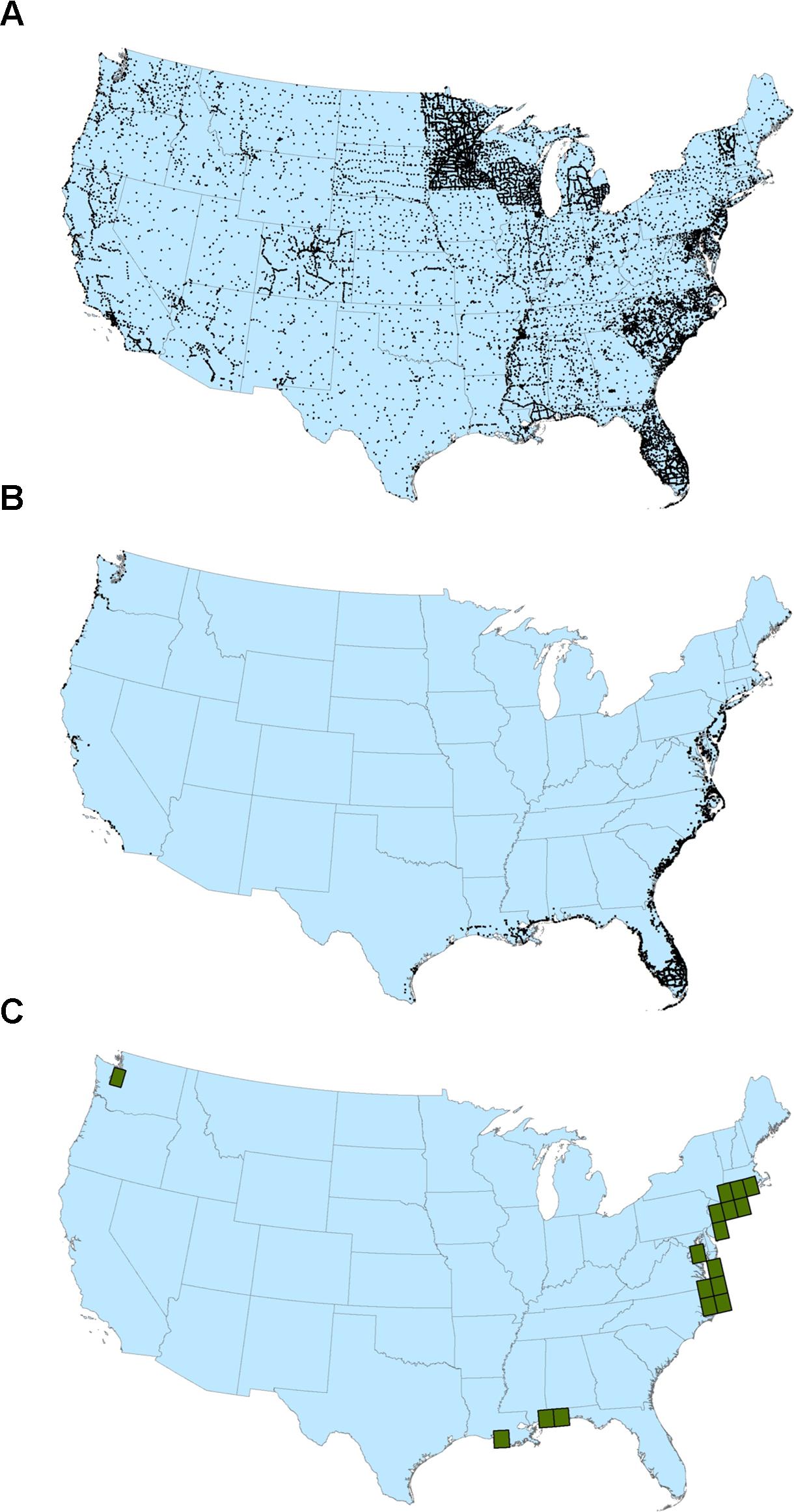
Figure 1. (A): GPS on Bench Marks reference data for CONUS (23,115 points); (B): Subset of reference data in the low elevation coastal zone (3,480 points); (C): Test area of 17 one-degree by one-degree tiles for direct DEM comparisons.
Results
The initial accuracy assessment was conducted on the DEMs for which coverage was available for all of CONUS: SRTM, ASTER GDEM (version 3), NED, and NED derived from lidar DEM source data (Gesch et al., 2014). Table 1 shows the accuracy assessment results for the full range of elevations across CONUS included in the reference data, as well as the results for only areas in the LECZ. The LECZ is defined as elevations less than or equal to 10 m above sea level, which is a commonly used elevation threshold to delimit coastal zones (McGranahan et al., 2007; Lichter et al., 2011; Neumann et al., 2015). For SRTM and ASTER GDEM, the elevation accuracy in the LECZ is degraded compared to the accuracy for all of CONUS, while for NED and NED with lidar source data, the accuracy is slightly improved in the LECZ. Because the primary interest for coastal assessments is in the low-lying areas subject to inundation and other adverse effects of increased water levels, the remainder of the results presented are for the LECZ. This approach follows the recommendation in other studies that emphasize accuracy testing with reference data representative of the area of interest to guard against overly optimistic results (Bolkas et al., 2016). Thus, limiting accuracy assessment to coastal areas (Du et al., 2015) is appropriate for this study.
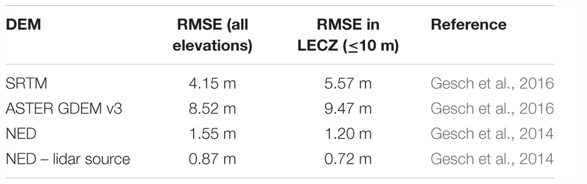
Table 1. Accuracy assessment results for DEMs over CONUS.
Vertical Accuracy and Inundation Assessment Parameters
Table 2 displays the accuracy information for DEMs over the CONUS LECZ. In addition to the four DEMs in Table 1, the specification for 3DEP lidar is added for comparison, as it represents high-resolution, high-accuracy elevation data being collected over broad areas in the U.S. 3DEP is an ongoing program of the U.S. Government to coordinate and collect enhanced elevation data for CONUS in an 8-year cycle (Sugarbaker et al., 2014). Most of the data are being collected to a specification for “quality level 2” (QL2), which requires a vertical RMSE of 0.10 m (Heidemann, 2012). The DEM accuracy metrics included in the table are RMSE, mean error, and mean absolute error (MAE). As noted above, mean error can be indicative of overall positive or negative bias in a DEM and, if a bias is present, can reflect a departure from a normal distribution of the errors (Maune et al., 2007). In these cases, the MAE can be a useful metric to help describe the error characteristics (Chai and Draxler, 2014). The positive mean errors for SRTM and ASTER GDEM do indicate that on average the DEMs are too high relative to the ground (as represented in the reference data point elevations) and the error distribution is not an unbiased normal distribution. The performance of SRTM and ASTER GDEM generally having a positive bias has been noted in previous published accuracy evaluations of these DEMs (Carabajal and Harding, 2006; Gesch et al., 2016).
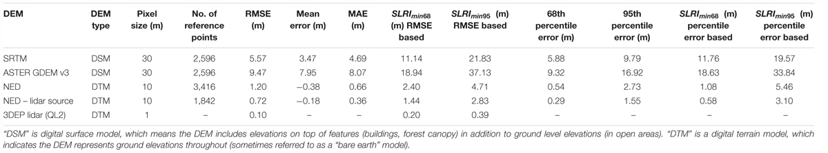
Table 2. DEM accuracy over CONUS LECZ.
In these cases of a biased error distribution, an alternative error metric to the RMSE (or its calculated equivalents like LE95) is a sample quantile of the cumulative error distribution (Höhle and Höhle, 2009), which has been widely implemented and used as the “95th percentile” error approach for describing the vertical accuracy (at the 95% confidence level) of DEMs with non-normal error distributions (Maune et al., 2007; ASPRS, 2015). Other sample quantiles can be used, for instance 68 or 90% (Wessel et al., 2018), for the percentile error metric. Table 2 includes both the 68th percentile and 95th percentile errors for each of the DEMs tested, along with the derived SLRImin measure, calculated from both the RMSE and percentile error metrics. For the percentile error metrics, the corresponding SLRImin measure is simply two times the percentile error. If a DEM accuracy validation is done for a specific area, then there is more flexibility in using the various error metrics to derive SLR assessment parameters (minimum increment and planning timeline), with the ability to deal with factors such as a biased non-normal error distribution with large outliers. In practice, most coastal assessments do not include DEM accuracy testing and characterization, but instead must rely upon DEMs with published accuracy figures, and RMSE is the only metric available with which to determine the proper increment and time horizon parameters. For this reason, comparisons of SLRImin and TLmin presented and discussed below are derived from the RMSE for the DEMs analyzed in this study.
Table 3 presents the results for the direct comparison of all the tested global DEMs within the 17 coastal test tile locations (Figure 1C). All the global DEMs exhibit accuracies that are better than their product specifications, as is often the case when these DEMs have been evaluated over broad areas. Refer to the tables in the Supplementary Material for a record of the numerous accuracy tests for SRTM (and its derivatives) (Supplementary Table S1), ASTER GDEM (Supplementary Table S2), AW3D30 (Supplementary Table S3), and TanDEM-X (Supplementary Table S4). Also included in the Supplementary Material are a summary of evaluations of NED (Supplementary Table S5), as an example of higher resolution DEMs with regional to national coverage, and a summary of example accuracies from technologies that produce very high-resolution and very high-accuracy elevation data that have been used in coastal assessments (Supplementary Table S6). The results in these tables provide context to the capabilities of global DEMs for coastal assessments and demonstrate the possibilities for very high-accuracy mapping when requirements call for detailed spatially explicit information.
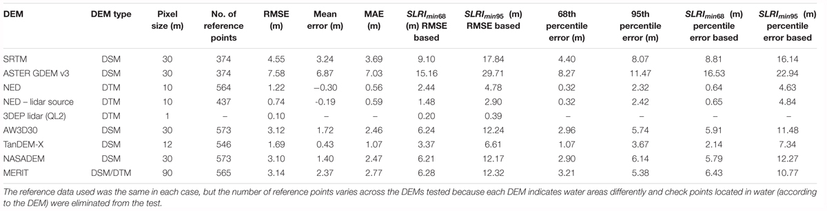
Table 3. DEM accuracy and corresponding SLRImin for LECZ areas within the 17 test tile locations.
Table 4 and Figure 2 show the evaluated DEMs ranked in order of increasing vertical uncertainty. The derived parameters of SLRImin and TLmin needed for coastal assessments have been calculated from the vertical accuracy for each DEM (as stated in the RMSE) and are presented at the 68 and 95% confidence levels. Included in the list of DEMs is terrestrial lidar, which is another example of a high-accuracy source of elevation data that can be used in detailed assessments. In this case, the vertical accuracy (RMSE = 0.05 m) comes from an example coastal DEM used for a flooding assessment on Kwajalein Atoll, RMI (Storlazzi, 2017). The results in Table 4 and Figure 2 indicate that only the high-resolution, high-accuracy DEM sources allow a SLRImin of less than 1 m and a TLmin of less than 100 years at high confidence levels, while the national scale or global DEMs do not adequately support such parameters.
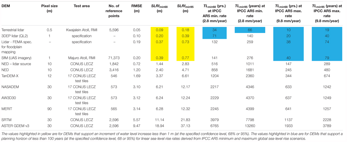
Table 4. Ranking of elevation data sources (in order of increasing RMSE) and corresponding SLRImin and TLmin for use in coastal assessments.
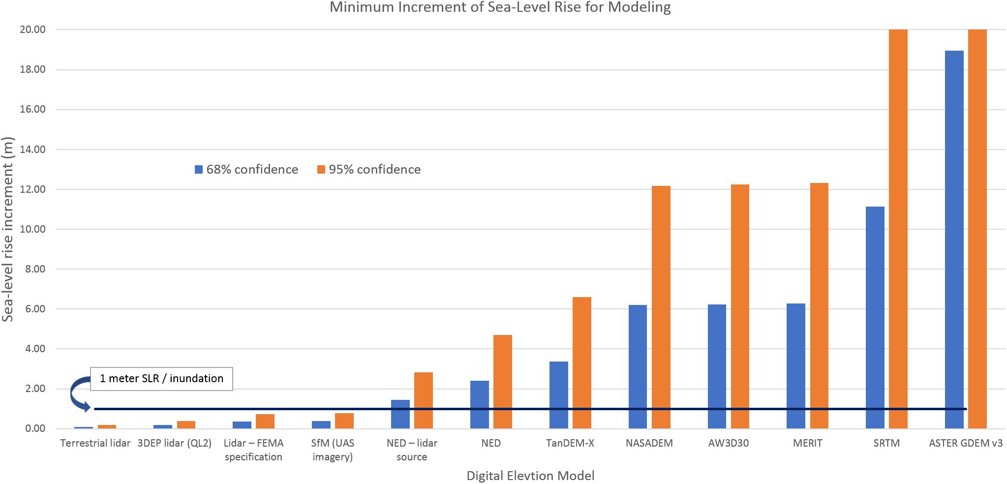
Figure 2. Ranking of elevation data sources (left to right in order of increasing SLRImin). The 1-m sea-level rise (or inundation level) is marked, which indicates that only the high-accuracy DEM sources are suitable for modeling sub-meter increments at high confidence levels.
Figure 3 shows how for a given DEM (and its associated vertical accuracy) the confidence level attached to SLRImin increases as the increment used for modeling increases. Note that when global DEMs and sub-meter increments of SLR (0.5 m or less) are used, the confidence is very low (in the 0–10% range). A simple formula for calculating the confidence level for SLRImin given the RMSE of the DEM and the modeled increment is described in the Supplementary Material.
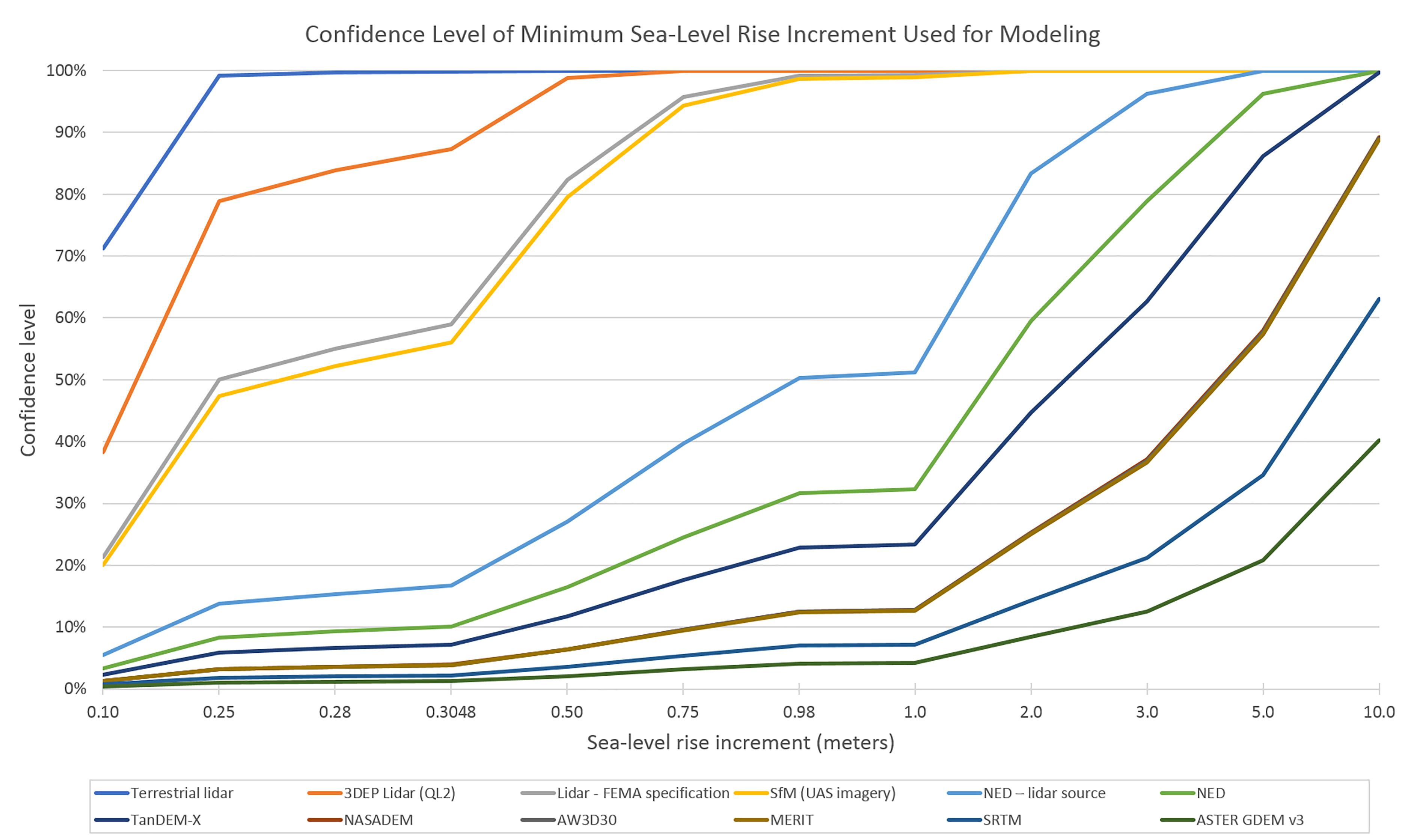
Figure 3. Confidence level for SLRImin for various DEMs and sea-level rise increments. Increments of 0.28 and 0.98 m are included because they represent the minimum and maximum scenarios, respectively, for global sea-level rise by the year 2100 as described in IPCC AR5 (Church et al., 2013). An increment of 0.3048 m is included because it is the equivalent of 1 foot, an increment that is commonly used in local and regional inundation assessments in the U.S.
Delineation of Low Elevation Coastal Zone
In addition to developing spatially explicit flooding or inundation impact zone maps, DEMs are also used to outline general LECZ delineations (McGranahan et al., 2007; Lichter et al., 2011; Neumann et al., 2015). Given the accuracy of global DEMs, and the corresponding SLRImin for each, the confidence levels for delineating the 10 m or less LECZ (that is, the 10-m elevation contour) and the 20 m or less coastal zone (CZ) (the 20-m contour) can be calculated (Table 5). The global DEMs suitable for delineating the LECZ (≤10 m elevation) at 68% confidence are TanDEM-X, CoastalDEM (an SRTM derivative) (Kulp and Strauss, 2018), NASADEM, AW3D30, and MERIT. At the 95% confidence level, only TanDEM-X is suitable for delineating the LECZ. All the global DEMs are acceptable for delineating the CZ (≤20 m elevation) at 68% confidence, while at the 95% confidence level SRTM and ASTER GDEM are no longer suitable, but the others are.
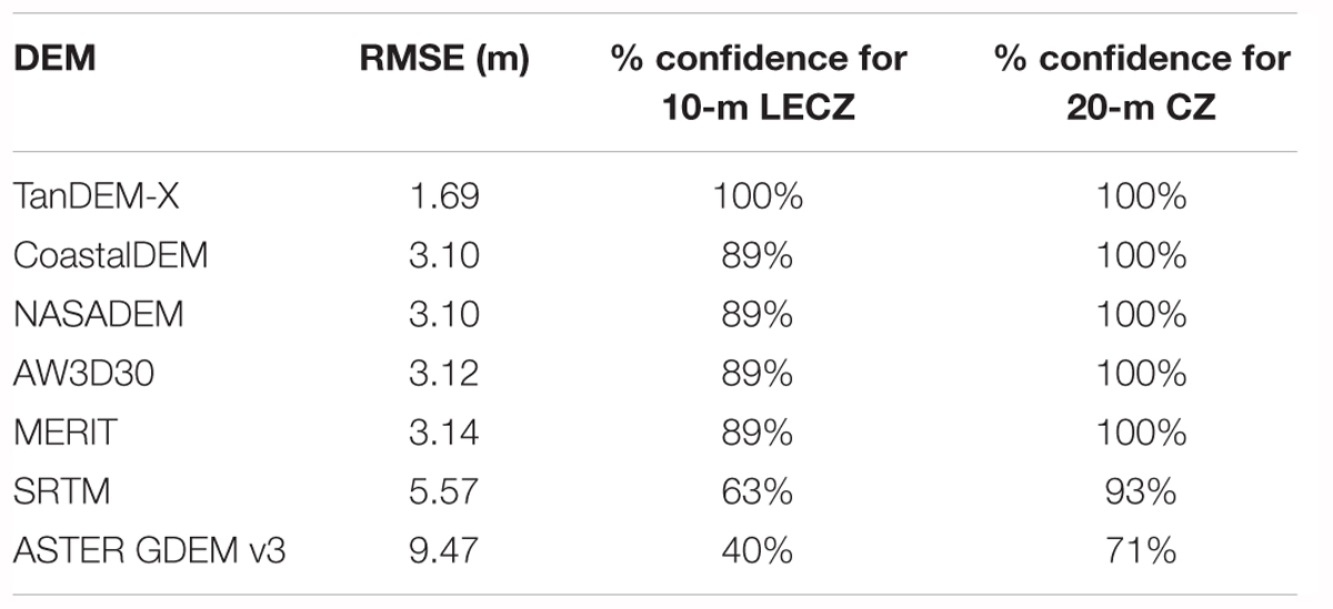
Table 5. The confidence level for delineating the 10-m LECZ and the 20-m coastal zone (CZ) using each global DEM.
Discussion
When the inherent vertical uncertainty is considered, it is clear that global DEMs are not adequate for modeling fine increments of SLR (<1 m) over short planning horizons (<100 years) at high confidence levels (Table 4). SLRImin and TLmin are easily calculated metrics based on the stated DEM accuracy (usually expressed as an RMSE) and are useful to quantify elevation-based coastal assessment parameters and their associated confidence levels. Numerous studies have used global DEMs for SLR and coastal flooding assessments without any regard for vertical uncertainty (elevation error), leading to large uncertainties in the assessment results with low confidence levels. There is ample evidence that SRTM and ASTER GDEM are severely limited for use in coastal assessments (Gesch, 2009; Gesch et al., 2009; van de Sande et al., 2012; Doyle et al., 2015; Griffin et al., 2015; Yan et al., 2015; Kulp and Strauss, 2016; Walczak et al., 2016; Yunus et al., 2016; Santillan and Makinano-Santillan, 2017; Smith et al., 2018). Both SRTM and ASTER GDEM are DSMs that generally overestimate elevations (especially in vegetated and built-up areas), so their use in coastal assessments leads to underestimating areas exposed to a given inundation level (van de Sande et al., 2012; Griffin et al., 2015; Kulp and Strauss, 2016; Smith et al., 2018). The results from the DEM accuracy assessment in this study (Table 3) do indicate the overestimation of elevation (positive bias) by SRTM and ASTER GDEM as reflected in the positive mean error for each. A bias (that is, a larger negative or positive mean error) is often an indicator that the error distribution is non-normal; therefore, applying linear scaling factors to the RMSE to derive LE90 or LE95 is not valid, so percentile error methods should be used (Maune et al., 2007; ASPRS, 2015). In the analysis presented here, the RMSE was used to derive SLRImin even when the DEMs had a positive bias, as often only the RMSE is known and the individual error values are not available for percentile error calculations. As shown in Table 3, however, SLRImin68 and SLRImin95 calculated based on the 68th percentile and 95th percentile errors, respectively, are not much different than those calculated based on the RMSE, so the finding that none of the global DEMs support an increment of 1 m is not changed.
There have been some recent improvements to SRTM (O’Loughlin et al., 2016; Kulp and Strauss, 2018; Moudrý et al., 2018) and ASTER GDEM (Arefi and Reinartz, 2011; Yang et al., 2018) by removing vegetation and other elevated features that caused the positive bias in the original datasets, often with the correction implemented by integrating Ice, Cloud and land Elevation Satellite (ICESat) spaceborne lidar data,. Merges of SRTM and ASTER GDEM (Satgé et al., 2015; Crippen et al., 2016; Yamazaki et al., 2017) have resulted in improved data as well. However, none of these improvements bring the DEMs to the level where they will support high confidence, quantitative coastal assessments with sub-meter water level change increments and planning horizons within the current century. The improvements to SRTM, namely CoastalDEM, NASADEM, and MERIT, all still have an RMSE of about 3 m, which equates to a minimum increment of more than 6 m at 68% confidence (Table 4 and Supplementary Table S1). AW3D30 is in this same class, with an RMSE of slightly more than 3 m (Table 4 and Supplementary Table S3). TanDEM-X does offer an improvement over SRTM, ASTER GDEM, and AW3D30 (Grohmann, 2018) and exhibits very little positive bias (Wessel et al., 2018), although its vertical error does result in a SLRImin of several meters (Table 4 and Supplementary Table S4).
Despite ample evidence of the significant limitations of global DEMs, especially SRTM, for coastal assessments, they have been used extensively for mapping and describing potential impacts of SLR and coastal flooding, often with assessment parameters (small water level increments and short planning horizons) that fall well within the error bounds of the underlying elevation data (Dasgupta et al., 2008, 2010; Hanson et al., 2010; Curtis and Schneider, 2011; Blankespoor et al., 2014; Hardy and Nuse, 2016; Kopp et al., 2017; Runting et al., 2017; Brown et al., 2018a,b; Gebremichael et al., 2018; Haer et al., 2018; Jevrejeva et al., 2018; Lincke and Hinkel, 2018; Nicholls et al., 2018; Prahl et al., 2018; Rasmussen et al., 2018; Schuerch et al., 2018; Wolff et al., 2018). Some of these studies used a model or database in which the global DEM is embedded, such as the Dynamic Interactive Vulnerability Assessment (DIVA) modeling framework (Hinkel, 2005; Vafeidis et al., 2008), so the inherent vertical uncertainty is contained within model or database components. This serves as a caution that even if a DEM is not a direct input or is not processed or analyzed directly in an inundation modeling exercise, vertical error may be implicit in sub-model or database components, thus modelers should be aware of an obscured source of uncertainty in their assessment. Some assessments have used even coarser global elevation models (1-km spatial resolution) with water level increments in the range of 0.3–2 m (Xingong et al., 2009; Nicholls et al., 2011; Brown et al., 2013; Neumann et al., 2015). All these assessments present statistics about the potential impact zones, including the areas and oftentimes the corresponding population and economic assets that are at risk of adverse effects. However, there is no quantitative statement about the quality of the reported results, for instance confidence level, and no expression of the uncertainty contributed by vertical error. In all cases, the water level change increments used in the assessments are not supported at high confidence levels, as the increments are very small compared to the DEM vertical error (and the derived minimum increment), which calls into question the veracity of the reported results. Reporting of inundated areas (and population and resources contained therein) at intervals of 1 m or less implies a degree of accuracy that is not present in global DEMs, and providing such numbers can be misleading to readers, especially because most will not be familiar with the concepts of vertical uncertainty of elevation models. As much as there is a desire and need for global SLR and coastal flooding analyses with water level increases on the order of a meter or less, current global DEMs do not have the requisite vertical accuracy to derive results with high confidence levels using fine increments, and thus they should not be used for such mapping.
Even though global DEMs are not appropriate for spatially explicit mapping of small increments of inundation with high confidence, they can be used effectively for delineation of general LECZs, and inventorying the population and resources contained within. As the RMSE improves for global DEMs, the confidence level for delineation of 10- and 20-m coastal zones increases (Table 5). The LECZ can be the framework for entire studies (McGranahan et al., 2007; Geisler and Currens, 2017), so a quality delineation of such a zone at a known confidence level is critical. For finer vertical slices, and subsequent spatially explicit exposure maps, much higher accuracy elevation data, such as that derived from lidar, high-resolution stereo photogrammetry, and ground survey, are required (Gallien et al., 2013). Airborne lidar, in particular, is an important elevation data source for coastal assessments (Gesch, 2009; Cooper et al., 2013; Runting et al., 2013; Zhu et al., 2015; Enwright et al., 2017), as it can meet the requirements for modeling fine increments of water level changes at high confidence and generally covers larger areas, even regional to national coverage.
Proper Accounting for Vertical Uncertainty
When vertical uncertainty is properly accounted for, value is added to the results of coastal assessments as additional information is available to inform users. For example, this can take the form of confidence levels attached to the inventory of resources within a potential impact zone or as portrayal of the probability of inundation for a specific location or confidence in the delineation of flooding exposure on a map. Several studies demonstrate best practices for handling cumulative vertical uncertainty in both the selection of assessment parameters (modeled increments and projection timelines) and in presentation of results (graphic and tabular) with expressions of confidence. For implementations of these best practices, see the following examples: Reynolds et al. (2012); Gesch (2013); Nielsen and Dudley (2013); Leon et al. (2014); Enwright et al. (2015, 2017); Dahl et al. (2017); Jones et al. (2017); Santillan and Makinano-Santillan (2017); West et al. (2018).
Other Inundation Exposure Assessment Best Practices
In addition to rigorous treatment of vertical uncertainty (detailed above in Section “Accounting for Uncertainty in Exposure Assessments” – spatial portrayal of cumulative vertical uncertainty when mapping inundation zones, and in Sections “Minimum Sea-Level Rise Increment” and “Minimum Planning Timeline” – selection of assessment parameters), there are other best practices that will help produce high quality coastal assessments. The following practices have emerged from the scientific record of successful studies, and they are becoming commonplace in the most robust assessments.
(1) In addition to delineation of areas of marine inundation (hydrologically connected to the ocean), delineate low-lying disconnected areas below the chosen elevation threshold. These areas have been referred to as locations with “groundwater inundation” (Rotzoll and Fletcher, 2012), although the inundation may not always be due solely to raised coastal groundwater tables, but also king tides, run-up of high waves, or some combination of these factors. The importance of distinct mapping of low-lying areas susceptible to flooding has been recognized in many studies (Cooper et al., 2012, 2013, 2015; Bloetscher and Romah, 2015; Bloetscher et al., 2017; Hummel et al., 2018; Knott et al., 2018). These delineations of low-lying lands should carry the same expression of confidence level of mapping or probability of inundation resulting from proper consideration of vertical uncertainty.
(2) Use spatially explicit regional relative SLR projections that account for the effects of vertical land movement. In contrast to global mean SLR scenarios, such projections capture the geographic variation in sea levels and can include factors such as ocean currents and changes in gravity fields (Wuebbles et al., 2017). The importance of using relative SLR rates is well recognized and demonstrated in numerous studies (Spada et al., 2013; Kopp et al., 2014; Nicholls et al., 2014; Slangen et al., 2014; Sweet and Park, 2014; Lentz et al., 2016; Wöppelmann and Marcos, 2016; Antonioli et al., 2017; Davis and Vinogradova, 2017; Gebremichael et al., 2018; Shirzaei and Bürgmann, 2018).
(3) Use dasymetric mapping if a coastal assessment includes estimates of impacted population. Many times, coastal assessments include an inventory of current and/or future population within the potential impact zone. Dasymetric population mapping (Mennis, 2003; Holt et al., 2004) is an effective technique for disaggregating areal population counts to a more realistic distribution of population density across the landscape as a continuous surface, often using land cover or parcel data as ancillary information. The advantages of doing so for coastal assessments have been demonstrated (Mitsova et al., 2012; Merkens and Vafeidis, 2018), and spatially explicit population maps are available over large areas (Mondal and Tatem, 2012; Dmowska and Stepinski, 2017).
Conclusion
Vertical uncertainty is a critical factor to consider and account for in elevation-based assessments of SLR and coastal flooding exposure. Some studies have properly handled the vertical uncertainty, as expressed in the combined elevation data and transformation errors, and in doing so provide valuable additional information to the user about confidence in the mapping and likelihood of projected impacts. However, many other studies ignore the vertical uncertainty stemming from the underlying elevation data and use assessment parameters (water level change increments and planning horizons) that are well within the error bounds and are not appropriate for generating high confidence results, thus leading to questionable delineations of impact zones and inventories of the population and resources contained therein.
The simple methods described herein for selecting coastal assessment parameters (minimum increment of water level change, SLRImin, and planning horizon, TLmin) that are supported at high confidence levels by the vertical qualities of the elevation data are useful for characterizing the capabilities of global DEMs. Application of these methods to current global DEMs (SRTM and its derivatives NASADEM, CoastalDEM, and MERIT; ASTER GDEM; AW3D30; and TanDEM-X) demonstrates that none of these DEMs support coastal inundation or flood assessment at high confidence levels for small water level increments (<1 m) or short planning horizons (<100 years). High confidence assessments of scenarios with cumulative SLR of less than 1 m or planning horizons within the current century require elevation data with much better vertical accuracy than that afforded by global DEMs, which points to high-accuracy sources such as terrestrial and airborne lidar, high-resolution photogrammetry, and ground surveys. These technologies produce high-quality elevation data that facilitate development of detailed spatially explicit inundation maps.
The key finding demonstrated in this study leads the list of best practices to follow in elevation-based coastal inundation assessments.
(1) Account for the inherent cumulative vertical uncertainty in the elevation data by using increments of water level increase and planning horizons that are supported at high confidence levels, and state those confidence levels explicitly in study documentation. The metrics SLRImin and TLmin are direct functions of the vertical accuracy of the DEM used in the study, and they are useful for ensuring that the chosen assessment parameters are appropriate given the error characteristics of the DEM.
(2) Apply probabilistic or modified deterministic methods when producing maps of impact zones and inventories of features and resources contained therein. These approaches allow for a specific probability or confidence level to be attached to the results, and ideally the maps portray that quality using clear symbology and the inventories are labeled with that information.
(3) Delineate impact zones above the normal high water line, which usually implies vertical datum transformation that should be reflected in cumulative vertical uncertainty (calculated via summing in quadrature).
(4) Enforce hydrologic connectivity (direct connection to the ocean) in the DEM when conducting spatially explicit mapping of marine inundation. Map and inventory separately the low-lying disconnected lands that are subject to flooding at the specified water level elevation.
(5) Use relative SLR rates that account for geographic variation and departures from global mean rates because of differential vertical land movement, ocean currents, and gravity.
(6) Employ dasymetric mapping techniques for better estimates of potential impacted population.
As the use of these best practices increases, assessments will improve and become more valuable, especially by having quantified and published uncertainty information (confidence levels and likelihood statements), and results will be directly comparable across different assessments.
In the future, as elevation datasets with large-area coverage improve, analyses utilizing the improved elevation information and the community best practices will result in robust assessments. Ongoing enhancements to widely used methods will also help to improve progress, such as better incorporation of information on physical processes, including tidal regimes (Hanslow et al., 2018) and water level attenuation due to surface roughness (Vafeidis et al., 2017), into bathtub modeling used for broad area screening. However, for elevation-based coastal assessments, the primary factor affecting quality and usefulness of results remains the choice of the elevation model used (National Oceanic and Atmospheric Administration [NOAA], 2010; Doyle et al., 2015; Wolff et al., 2016; Yunus et al., 2016), and how the DEM vertical uncertainty is characterized and accounted for (West et al., 2018). Open-access global DEMs have been a major advance for many Earth science and environmental modeling applications, but the findings from the present evaluation of currently available datasets for detailed assessments of SLR and coastal flooding exposure add to the recent recognition (Schumann et al., 2014; Simpson et al., 2015; Sampson et al., 2016) that the requirement remains for a freely available, high-accuracy, high-resolution global elevation model that supports quantitative coastal inundation hazard assessments at high confidence levels.
Data Availability Statement
All data generated or analyzed during this study are included in the main text of this publication.
Author Contributions
DG designed the study, performed the data collection, processing, and analysis, and wrote the manuscript.
Funding
Funding for this research was provided by the Land Change Science Program of the U.S. Geological Survey. TanDEM-X data (©DLR 2017) were provided by the German Aerospace Center (DLR) through the TanDEM-X Digital Elevation Model Announcement of Opportunity (Proposal ID: DEM_HYDR1176).
Conflict of Interest Statement
The author declares that the research was conducted in the absence of any commercial or financial relationships that could be construed as a potential conflict of interest.
Acknowledgments
The author thanks Monica Palaseanu-Lovejoy for valuable comments on an earlier version of the manuscript. Any use of trade, firm, or product names is for descriptive purposes only and does not imply endorsement by the U.S. Government.
Supplementary Material
The Supplementary Material for this article can be found online at: https://www.frontiersin.org/articles/10.3389/feart.2018.00230/full#supplementary-material
Footnotes
- ^ https://vdatum.noaa.gov/docs/est_uncertainties.html
- ^ https://www.ngs.noaa.gov/GEOID/GEOID12B/GPSonBM12B.shtml
References
Abrams, M., Bailey, B., Tsu, H., and Hato, M. (2010). The ASTER global DEM. Photogramm. Eng. Remote Sensing 76, 344–348.
Antonioli, F., Anzidei, M., Amorosi, A., Lo Presti, V., Mastronuzzi, G., Deiana, G., et al. (2017). Sea-level rise and potential drowning of the Italian coastal plains: flooding risk scenarios for 2100. Quat. Sci. Rev. 158, 29–43. doi: 10.1016/j.quascirev.2016.12.021
Arefi, H., and Reinartz, P. (2011). Accuracy enhancement of ASTER global digital elevation models using ICESat data. Remote Sensing 3, 1323–1343. doi: 10.3390/rs3071323
ASPRS (2015). ASPRS positional accuracy standards for digital geospatial data. Photogramm. Eng. Remote Sensing 81, A1–A26. doi: 10.14358/PERS.81.3.A1-A26
Bales, J. D., and Wagner, C. R. (2009). Sources of uncertainty in flood inundation maps. J. Flood Risk Manag. 2, 139–147. doi: 10.1111/j.1753-318X.2009.01029.x
Bates, P. D., and De Roo, A. P. J. (2000). A simple raster-based model for flood inundation simulation. J. Hydrol. 236, 54–77. doi: 10.1016/S0022-1694(00)00278-X
Bell, J., Saunders, M. I., Leon, J. X., Mills, M., Kythreotis, A., Phinn, S., et al. (2014). Maps, laws and planning policy: working with biophysical and spatial uncertainty in the case of sea level rise. Environ. Sci. Policy 44, 247–257. doi: 10.1016/j.envsci.2014.07.018
Blankespoor, B., Dasgupta, S., and Laplante, B. (2014). Sea-level rise and coastal wetlands. Ambio 43, 996–1005. doi: 10.1007/s13280-014-0500-4
Bloetscher, F., and Romah, T. (2015). Tools for assessing sea level rise vulnerability. J. Water Clim. Change 6, 181–190. doi: 10.1007/s11625-016-0357-5
Bloetscher, F., Sairam, N., Nagarajan, S., Berry, L., and Hoermann, S. (2017). Assessing sea level rise vulnerability and costs in a data limited environment. Int. J. Eng. Technol. Manag. Res. 4, 13–31. doi: 10.5281/zenodo.844078
Bolkas, D., Fotopoulos, G., Braun, A., and Tziavos, I. N. (2016). Assessing digital elevation model uncertainty using GPS survey data. J. Surv. Eng. 142:04016001. doi: 10.1061/(ASCE)SU.1943-5428.0000169
Boyd, E., Pasquantonio, V., Rabalais, F., and Eustis, S. (2016). Although critical, carbon choices alone do not determine the fate of coastal cities. Proc. Natl. Acad. Sci. U.S.A. 113:E1329. doi: 10.1073/pnas.1525067113
Brown, S., Nicholls, R. J., Goodwin, P., Haigh, I. D., Lincke, D., Vafeidis, A. T., et al. (2018a). Quantifying land and people exposed to sea-level rise with no mitigation and 1.5°C and 2.0°C rise in global temperatures to year 2300. Earths Future 6, 583–600. doi: 10.1002/2017ef000738
Brown, S., Nicholls, R. J., Lázár, A. N., Hornby, D. D., Hill, C., Hazra, S., et al. (2018b). What are the implications of sea-level rise for a 1.5, 2 and 3°C rise in global mean temperatures in the Ganges-Brahmaputra-Meghna and other vulnerable deltas? Reg. Environ. Change 18, 1829–1842. doi: 10.1007/s10113-018-1311-0
Brown, S., Nicholls, R. J., Lowe, J. A., and Hinkel, J. (2013). Spatial variations of sea-level rise and impacts: an application of DIVA. Clim. Change 134, 403–416. doi: 10.1007/s10584-013-0925-y
Carabajal, C. C., and Harding, D. J. (2006). SRTM C-band and ICESat laser altimetry elevation comparisons as a function of tree cover and relief. Photogramm. Eng. Remote Sensing 72, 287–298. doi: 10.14358/PERS.72.3.287
Chai, T., and Draxler, R. R. (2014). Root mean square error (RMSE) or mean absolute error (MAE)? – Arguments against avoiding RMSE in the literature. Geosci. Model Dev. 7, 1247–1250. doi: 10.5194/gmd-7-1247-2014
Church, J. A., Clark, P. U., Cazenave, A., Gregory, J. M., Jevrejeva, S., Levermann, A., et al. (2013). “Sea level change,” in Climate Change 2013: The Physical Science Basis: Working Group I Contribution to the Fifth Assessment Report of the Intergovernmental Panel on Climate Change, eds T. F. Stocker, D. Qin, G.-K. Plattner, M. Tignor, S. K. Allen, J. Boschung, et al. (Cambridge: Cambridge University Press), 1137–1216. doi: 10.1017/CBO9781107415324.026
Cooper, H. M., and Chen, Q. (2013). Incorporating uncertainty of future sea-level rise estimates into vulnerability assessment: a case study in Kahului, Maui. Clim. Change 121, 635–647. doi: 10.1007/s10584-013-0987-x
Cooper, H. M., Chen, Q., Fletcher, C. H., and Barbee, M. M. (2012). Assessing vulnerability due to sea-level rise in Maui, Hawai‘i using LiDAR remote sensing and GIS. Clim. Change 116, 547–563. doi: 10.1007/s10584-012-0510-9
Cooper, H. M., Fletcher, C. H., Chen, Q., and Barbee, M. M. (2013). Sea-level rise vulnerability mapping for adaptation decisions using LiDAR DEMs. Prog. Phys. Geogr. 37, 745–766. doi: 10.1177/0309133313496835
Cooper, H. M., Zhang, C., and Selch, D. (2015). Incorporating uncertainty of groundwater modeling in sea-level rise assessment: a case study in South Florida. Clim. Change 129, 281–294. doi: 10.1007/s10584-015-1334-1
Coveney, S., and Fotheringham, A. S. (2011). The impact of DEM data source on prediction of flooding and erosion risk due to sea-level rise. Int. J. Geogr. Inf. Sci. 25, 1191–1211. doi: 10.1080/13658816.2010.545064
Crippen, R., Buckley, S., Agram, P., Belz, E., Gurrola, E., Hensley, S., et al. (2016). NASADEM global elevation model: methods and progress. Int. Arch. Photogramm. Remote Sens. Spatial Inf. Sci. XLI-B4, 125–128. doi: 10.5194/isprs-archives-XLI-B4-125-2016
Curtis, K. J., and Schneider, A. (2011). Understanding the demographic implications of climate change: estimates of localized population predictions under future scenarios of sea-level rise. Popul. Environ. 33, 28–54. doi: 10.1007/s11111-011-0136-2
Dahl, K. A., Spanger-Siegfried, E., Caldas, A., and Udvardy, S. (2017). Effective inundation of continental United States communities with 21st century sea level rise. Elementa Sci. Anthropocene 5:37. doi: 10.1525/elementa.234
Dasgupta, S., Laplante, B., Meisner, C., Wheeler, D., and Yan, J. (2008). The impact of sea level rise on developing countries: a comparative analysis. Clim. Change 93, 379–388. doi: 10.1007/s10584-008-9499-5
Dasgupta, S., Laplante, B., Murray, S., and Wheeler, D. (2010). Exposure of developing countries to sea-level rise and storm surges. Clim. Change 106, 567–579. doi: 10.1007/s10584-010-9959-6
Davis, J. L., and Vinogradova, N. T. (2017). Causes of accelerating sea level on the East Coast of North America. Geophys. Res. Lett. 44, 5133–5141. doi: 10.1002/2017gl072845
Dmowska, A., and Stepinski, T. F. (2017). A high resolution population grid for the conterminous United States: the 2010 edition. Comput. Environ. Urban Syst. 61, 13–23. doi: 10.1016/j.compenvurbsys.2016.08.006
Doyle, T. W., Chivoiu, B., and Enwright, N. M. (2015). “Sea-level rise modeling handbook: resource guide for coastal land managers, engineers, and scientists,” in USGS Professional Paper 1815, (Reston, VA: USGS), doi: 10.3133/pp1815
Du, X., Guo, H., Fan, X., Zhu, J., Yan, Z., and Zhan, Q. (2015). Vertical accuracy assessment of freely available digital elevation models over low-lying coastal plains. Int. J. Digit. Earth 9, 252–271. doi: 10.1080/17538947.2015.1026853
Emrich, C. T., and Cutter, S. L. (2011). Social vulnerability to climate-sensitive hazards in the Southern United States. Weather Clim. Soc. 3, 193–208. doi: 10.1175/2011WCAS1092.1
Enwright, N., Wang, L., Borchert, S., Day, R., Feher, L., and Osland, M. (2017). The impact of lidar elevation uncertainty on mapping intertidal habitats on barrier islands. Remote Sens. 10:5. doi: 10.3390/rs10010005
Enwright, N. M., Griffith, K. T., and Osland, M. J. (2015). “Incorporating future change into current conservation planning: evaluating tidal saline wetland migration along the U.S. Gulf of Mexico coast under alternative sea-level rise and urbanization scenarios,” in USGS Data Series 969, (Reston, VA: USGS), doi: 10.3133/ds969
Ericson, J., Vorosmarty, C., Dingman, S., Ward, L., and Meybeck, M. (2006). Effective sea-level rise and deltas: causes of change and human dimension implications. Glob. Planet. Change 50, 63–82. doi: 10.1016/j.gloplacha.2005.07.004
Farr, T. G., Rosen, P. A., Caro, E., Crippen, R., Duren, R., Hensley, S., et al. (2007). The shuttle radar topography mission. Rev. Geophys. 45:RG2004. doi: 10.1029/2005rg000183
Fereshtehpour, M., and Karamouz, M. (2018). DEM resolution effects on coastal flood vulnerability assessment: deterministic and probabilistic approach. Water Resour. Res. 54, 4965–4982. doi: 10.1029/2017wr022318
Fisher, P. (1998). Improved modeling of elevation error with Geostatistics. Geoinformatica 2, 215–233. doi: 10.1023/A:1009717704255
Fisher, P. F., and Tate, N. J. (2006). Causes and consequences of error in digital elevation models. Prog. Phys. Geogr. 30, 467–489. doi: 10.1191/0309133306pp492ra
Fraile-Jurado, P., and Ojeda-Zújar, J. (2012). The importance of the vertical accuracy of digital elevation models in gauging inundation by sea level rise along the Valdelagrana beach and marshes (Bay of Cádiz, SW Spain). Geo Mar. Lett. 33, 225–230. doi: 10.1007/s00367-012-0317-8
Gallien, T. W., Barnard, P. L., Van Ormondt, M., Foxgrover, A. C., and Sanders, B. F. (2013). A parcel-scale coastal flood forecasting prototype for a southern California urbanized embayment. J. Coast. Res. 288, 642–656. doi: 10.2112/jcoastres-d-12-00114.1
Gallien, T. W., Sanders, B. F., and Flick, R. E. (2014). Urban coastal flood prediction: integrating wave overtopping, flood defenses and drainage. Coast. Eng. 91, 18–28. doi: 10.1016/j.coastaleng.2014.04.007
Gallien, T. W., Schubert, J. E., and Sanders, B. F. (2011). Predicting tidal flooding of urbanized embayments: a modeling framework and data requirements. Coast. Eng. 58, 567–577. doi: 10.1016/j.coastaleng.2011.01.011
Gebremichael, E., Sultan, M., Becker, R., El Bastawesy, M., Cherif, O., and Emil, M. (2018). Assessing land deformation and sea encroachment in the Nile delta: a radar interferometric and inundation modeling approach. J. Geophys. Res. Solid Earth 123, 3208–3224. doi: 10.1002/2017jb015084
Geisler, C., and Currens, B. (2017). Impediments to inland resettlement under conditions of accelerated sea level rise. Land Use Policy 66, 322–330. doi: 10.1016/j.landusepol.2017.03.029
Gesch, D., Oimoen, M., Danielson, J., and Meyer, D. (2016). Validation of the ASTER global digital elevation model version 3 over the conterminous United States. Int. Arch. Photogramm. Remote Sens. Spatial Inf. Sci. XLI-B4, 143–148. doi: 10.5194/isprs-archives-XLI-B4-143-2016
Gesch, D. B. (2007). “The National Elevation Dataset,” in Digital Elevation Model Technologies and Applications: The DEM Users Manual, 2nd Edn, ed. D. F. Maune (Bethesda, MD: American Society for Photogrammetry and Remote Sensing), 99–118.
Gesch, D. B. (2009). Analysis of lidar elevation data for improved identification and delineation of lands vulnerable to sea-level rise. J. Coast. Res. 10053, 49–58. doi: 10.2112/si53-006.1
Gesch, D. B. (2012a). “Elevation uncertainty in coastal inundation hazard assessments,” in Natural Disasters, ed. S. Cheval (Vukovar: InTech), 121–140. doi: 10.5772/31972
Gesch, D. B. (2012b). “Global digital elevation model development from satellite remote-sensing data,” in Advances in Mapping from Remote Sensor Imagery—Techniques and Applications, eds X. Yang and J. Li (Boca Raton. FL: CRC Press), 91–117.
Gesch, D. B. (2013). Consideration of vertical uncertainty in elevation-based sea-level rise assessments: Mobile Bay, Alabama case study. J. Coast. Res. 63, 197–210. doi: 10.2112/si63-016.1
Gesch, D. B., Gutierrez, B. T., and Gill, S. K. (2009). “Coastal elevations,” in Coastal Sensitivity to Sea Level Rise—a Focus on the Mid-Atlantic Region. A Report, eds J. G. Titus, K. E. Anderson, D. R. Cahoon, D. B. Gesch, S. K. Gill, B. T. Gutierrez, et al. (Washington, DC: U.S. Climate Change Science Program).
Gesch, D. B., Oimoen, M., Greenlee, S. K., Nelson, C. A., Steuck, M., and Tyler, D. (2002). The National Elevation Dataset. Photogramm. Eng. Remote Sensing 68, 5–11.
Gesch, D. B., Oimoen, M. J., and Evans, G. A. (2014). “Accuracy assessment of the U.S. Geological Survey National Elevation Dataset, and comparison with other large-area elevation datasets: SRTM and ASTER,” in USGS Open-File Report 2014-1008, (Reston, VA: USGS), doi: 10.3133/ofr20141008
Gilmer, B., and Ferdaña, Z. (2012). “Developing a framework for assessing coastal vulnerability to sea level rise in southern New England, USA,” in Resilient Cities 2, Local Sustainability, Vol. 2, ed. K. Otto-Zimmermann (Dordrecht: Springer), 25–36. doi: 10.1007/978-94-007-4223-9_4
Griffin, J., Latief, H., Kongko, W., Harig, S., Horspool, N., Hanung, R., et al. (2015). An evaluation of onshore digital elevation models for modeling tsunami inundation zones. Front. Earth Sci. 3:32. doi: 10.3389/feart.2015.00032
Grohmann, C. H. (2018). Evaluation of TanDEM-X DEMs on selected Brazilian sites: comparison with SRTM, ASTER GDEM and ALOS AW3D30. Remote Sens. Environ. 212, 121–133. doi: 10.1016/j.rse.2018.04.043
Habel, S., Fletcher, C. H., Rotzoll, K., and El-Kadi, A. I. (2017). Development of a model to simulate groundwater inundation induced by sea-level rise and high tides in Honolulu, Hawaii. Water Res. 114, 122–134. doi: 10.1016/j.watres.2017.02.035
Haer, T., Botzen, W. J. W., Van Roomen, V., Connor, H., Zavala-Hidalgo, J., Eilander, D. M., et al. (2018). Coastal and river flood risk analyses for guiding economically optimal flood adaptation policies: a country-scale study for Mexico. Philos. Trans. A Math. Phys. Eng. Sci. 376:20170329. doi: 10.1098/rsta.2017.0329
Haer, T., Kalnay, E., Kearney, M., and Moll, H. (2013). Relative sea-level rise and the conterminous United States: consequences of potential land inundation in terms of population at risk and GDP loss. Glob. Environ. Change 23, 1627–1636. doi: 10.1016/j.gloenvcha.2013.09.005
Hanslow, D. J., Morris, B. D., Foulsham, E., and Kinsela, M. A. (2018). A regional scale approach to assessing current and potential future exposure to tidal inundation in different types of estuaries. Sci. Rep. 8:7065. doi: 10.1038/s41598-018-25410-y
Hanson, S., Nicholls, R., Ranger, N., Hallegatte, S., Corfee-Morlot, J., Herweijer, C., et al. (2010). A global ranking of port cities with high exposure to climate extremes. Clim. Change 104, 89–111. doi: 10.1007/s10584-010-9977-4
Hardy, R. D., and Nuse, B. L. (2016). Global sea-level rise: weighing country responsibility and risk. Clim. Change 137, 333–345. doi: 10.1007/s10584-016-1703-4
Heidemann, H. K. (2012). “Lidar base specification,” in USGS Techniques and Methods 11-B4: National Geospatial Program, Edn Version 1.0: Originally posted August 17. 2012; Version 1.1: October 29, 2014; Version 1.2: November 12, 2014; Version 1.3: February 28, 2018 (Reston, VA: U.S. Geological Survey). doi: 10.3133/tm11B4
Hinkel, J. (2005). DIVA: an iterative method for building modular integrated models. Adv. Geosci. 4, 45–50. doi: 10.5194/adgeo-4-45-2005
Hinkel, J., Lincke, D., Vafeidis, A. T., Perrette, M., Nicholls, R. J., Tol, R. S. J., et al. (2014). Coastal flood damage and adaptation costs under 21st century sea-level rise. Proc. Natl. Acad. Sci. U.S.A. 111, 3292–3297. doi: 10.1073/pnas.1222469111
Höhle, J., and Höhle, M. (2009). Accuracy assessment of digital elevation models by means of robust statistical methods. ISPRS J. Photogramm. Remote Sens. 64, 398–406. doi: 10.1016/j.isprsjprs.2009.02.003
Holt, J. B., Lo, C. P., and Hodler, T. W. (2004). Dasymetric estimation of population density and areal interpolation of census data. Cartogr. Geogr. Inf. Sci. 31, 103–121. doi: 10.1559/1523040041649407
Hummel, M. A., Berry, M. S., and Stacey, M. T. (2018). Sea level rise impacts on wastewater treatment systems along the U.S. Coasts. Earths Future 6, 622–633. doi: 10.1002/2017EF000805
Hunter, G. J., and Goodchild, M. F. (1995). Dealing with error in spatial databases: a simple case study. Photogramm. Eng. Remote Sensing 61, 529–537.
Jevrejeva, S., Jackson, L. P., Grinsted, A., Lincke, D., and Marzeion, B. (2018). Flood damage costs under the sea level rise with warming of 1.5°C and 2°C. Environ. Res. Lett. 13:074014. doi: 10.1088/1748-9326/aacc76
Jones, J. M., Henry, K., Wood, N., Ng, P., and Jamieson, M. (2017). HERA: a dynamic web application for visualizing community exposure to flood hazards based on storm and sea level rise scenarios. Comput. Geosci. 109, 124–133. doi: 10.1016/j.cageo.2017.08.012
Kettle, N. P. (2012). Exposing compounding uncertainties in sea level rise assessments. J. Coast. Res. 279, 161–173. doi: 10.2112/jcoastres-d-10-00011.1
Knott, J. F., Daniel, J. S., Jacobs, J. M., and Kirshen, P. (2018). Adaptation planning to mitigate coastal-road pavement damage from groundwater rise caused by sea-level rise. Transp. Res. Rec. doi: 10.1177/0361198118757441
Kopp, R. E., Deconto, R. M., Bader, D. A., Hay, C. C., Horton, R. M., Kulp, S., et al. (2017). Evolving understanding of Antarctic ice-sheet physics and ambiguity in probabilistic sea-level projections. Earths Future 5, 1217–1233. doi: 10.1002/2017ef000663
Kopp, R. E., Horton, R. M., Little, C. M., Mitrovica, J. X., Oppenheimer, M., Rasmussen, D. J., et al. (2014). Probabilistic 21st and 22nd century sea-level projections at a global network of tide-gauge sites. Earths Future 2, 383–406. doi: 10.1002/2014ef000239
Kostelnick, J. C., McDermott, D., Rowley, R. J., and Bunnyfield, N. (2013). A cartographic framework for visualizing risk. Cartographica Int. J. Geogr. Inf. Geovisual. 48, 200–224. doi: 10.3138/carto.48.3.1531
Kovanen, J., Oksanen, J., and Sarjakoski, T. (2018). Near real-time coastal flood inundation simulation with uncertainty analysis and GPU acceleration in a web environment. Comput. Geosci. 119, 39–48. doi: 10.1016/j.cageo.2018.06.007
Kuhn, M., Tuladhar, D., and Corner, R. (2011). Visualising the spatial extent of predicted coastal zone inundation due to sea level rise in south-west Western Australia. Ocean Coast. Manag. 54, 796–806. doi: 10.1016/j.ocecoaman.2011.08.005
Kulp, S., and Strauss, B. H. (2016). Global DEM errors underpredict coastal vulnerability to sea level rise and flooding. Front. Earth Sci. 4:36. doi: 10.3389/feart.2016.00036
Kulp, S., and Strauss, B. H. (2017). Rapid escalation of coastal flood exposure in US municipalities from sea level rise. Clim. Change 142, 477–489. doi: 10.1007/s10584-017-1963-7
Kulp, S. A., and Strauss, B. H. (2018). CoastalDEM: a global coastal digital elevation model improved from SRTM using a neural network. Remote Sens. Environ. 206, 231–239. doi: 10.1016/j.rse.2017.12.026
Le Cozannet, G., Nicholls, R., Hinkel, J., Sweet, W., McInnes, K., Van De Wal, R., et al. (2017). Sea level change and coastal climate services: the way forward. J. Mar. Sci. Eng. 5:49. doi: 10.3390/jmse5040049
Le Cozannet, G., Rohmer, J., Cazenave, A., Idier, D., van de Wal, R., de Winter, R., et al. (2015). Evaluating uncertainties of future marine flooding occurrence as sea-level rises. Environ. Model. Softw. 73, 44–56. doi: 10.1016/j.envsoft.2015.07.021
Lentz, E. E., Thieler, E. R., Plant, N. G., Stippa, S. R., Horton, R. M., and Gesch, D. B. (2016). Evaluation of dynamic coastal response to sea-level rise modifies inundation likelihood. Nat. Clim. Change 6, 696–700. doi: 10.1038/nclimate2957
Leon, J. X., Heuvelink, G. B. M., and Phinn, S. R. (2014). Incorporating DEM uncertainty in coastal inundation mapping. PLoS One 9:e108727. doi: 10.1371/journal.pone.0108727
Lichter, M., Vafeidis, A. T., Nicholls, R. J., and Kaiser, G. (2011). Exploring data-related uncertainties in analyses of land area and population in the “Low-Elevation Coastal Zone” (LECZ). J. Coast. Res. 274, 757–768. doi: 10.2112/jcoastres-d-10-00072.1
Lincke, D., and Hinkel, J. (2018). Economically robust protection against 21st century sea-level rise. Glob. Environ. Change 51, 67–73. doi: 10.1016/j.gloenvcha.2018.05.003
Maloney, M. C., and Preston, B. L. (2014). A geospatial dataset for U.S. hurricane storm surge and sea-level rise vulnerability: development and case study applications. Clim. Risk Manag. 2, 26–41. doi: 10.1016/j.crm.2014.02.004
Marbaix, P., and Nicholls, R. J. (2007). Accurately determining the risks of rising sea level. Eos 88, 441–442. doi: 10.1029/2007EO430002
Maune, D. F., Maitra, J. B., and McKay, E. J. (2007). “Accuracy standards & guidelines,” in Digital Elevation Model Technologies and Applications: The DEM Users Manual, 2nd Edn, ed. D. F. Maune (Bethesda, MD: American Society for Photogrammetry and Remote Sensing), 65–97.
McGranahan, G., Balk, D., and Anderson, B. (2007). The rising tide: assessing the risks of climate change and human settlements in low elevation coastal zones. Environ. Urban. 19, 17–37. doi: 10.1177/0956247807076960
Mcleod, E., Hinkel, J., Vafeidis, A. T., Nicholls, R. J., Harvey, N., and Salm, R. (2010). Sea-level rise vulnerability in the countries of the Coral Triangle. Sustain. Sci. 5, 207–222. doi: 10.1007/s11625-010-0105-1
Mennis, J. (2003). Generating surface models of population using dasymetric mapping. Prof. Geogr. 55, 31–42. doi: 10.1111/0033-0124.10042
Merkens, J.-L., and Vafeidis, A. (2018). Using information on settlement patterns to improve the spatial distribution of population in coastal impact assessments. Sustainability 10:3170. doi: 10.3390/su10093170
Mitsova, D., Esnard, A.-M., and Li, Y. (2012). Using enhanced dasymetric mapping techniques to improve the spatial accuracy of sea level rise vulnerability assessments. J. Coast. Conserv. 16, 355–372. doi: 10.1007/s11852-012-0206-3
Mogensen, L. A., and Rogers, K. (2018). Validation and comparison of a model of the effect of sea-level rise on coastal wetlands. Sci. Rep. 8:1369. doi: 10.1038/s41598-018-19695-2
Mondal, P., and Tatem, A. J. (2012). Uncertainties in measuring populations potentially impacted by sea level rise and coastal flooding. PLoS One 7:e48191. doi: 10.1371/journal.pone.0048191
Moudrý, V., Lecours, V., Gdulová, K., Gábor, L., Moudrá, L., Kropáček, J., et al. (2018). On the use of global DEMs in ecological modelling and the accuracy of new bare-earth DEMs. Ecol. Model. 383, 3–9. doi: 10.1016/j.ecolmodel.2018.05.006
National Oceanic and Atmospheric Administration [NOAA] (2010). “Technical considerations for use of geospatial data in sea level change mapping and assessment,” in NOAA Technical Report NOS 2010-01, (Silver Spring, MD: NOAA).
Neumann, B., Vafeidis, A. T., Zimmermann, J., and Nicholls, R. J. (2015). Future coastal population growth and exposure to sea-level rise and coastal flooding–a global assessment. PLoS One 10:e0118571. doi: 10.1371/journal.pone.0118571
Nicholls, R. J., Brown, S., Goodwin, P., Wahl, T., Lowe, J., Solan, M., et al. (2018). Stabilization of global temperature at 1.5 degrees C and 2.0 degrees C: implications for coastal areas. Philos. Trans. A Math. Phys. Eng. Sci. 376:20160448. doi: 10.1098/rsta.2016.0448
Nicholls, R. J., Hanson, S. E., Lowe, J. A., Warrick, R. A., Lu, X., and Long, A. J. (2014). Sea-level scenarios for evaluating coastal impacts. Wiley Interdiscip. Rev. Clim. Change 5, 129–150. doi: 10.1002/wcc.253
Nicholls, R. J., Marinova, N., Lowe, J. A., Brown, S., Vellinga, P., De Gusmao, D., et al. (2011). Sea-level rise and its possible impacts given a ‘beyond 4 degrees C world’ in the twenty-first century. Philos. Trans. A Math. Phys. Eng. Sci. 369, 161–181. doi: 10.1098/rsta.2010.0291
Nielsen, M. G., and Dudley, R. W. (2013). “Estimates of future inundation of salt marshes in response to sea-level rise in and around Acadia National Park, Maine,” in USGS Scientific Investigations Report 2012-5290, (Reston, VA: USGS).
O’Loughlin, F. E., Paiva, R. C. D., Durand, M., Alsdorf, D. E., and Bates, P. D. (2016). A multi-sensor approach towards a global vegetation corrected SRTM DEM product. Remote Sens. Environ. 182, 49–59. doi: 10.1016/j.rse.2016.04.018
Palaseanu-Lovejoy, M., Poppenga, S. K., Danielson, J. J., Tyler, D. J., Gesch, D. B., Kottermair, M., et al. (2018). “One-meter topobathymetric digital elevation model for Majuro atoll, Republic of the Marshall Islands, 1944 to 2016,” in USGS Scientific Investigations Report 2018-5047, (Reston, VA: USGS), doi: 10.3133/sir20185047
Paprotny, D., Morales-Nápoles, O., Vousdoukas, M. I., Jonkman, S. N., and Nikulin, G. (2018). Accuracy of pan-European coastal flood mapping. J. Flood Risk Manag. e12459. doi: 10.1111/jfr3.12459
Parker, B., Hess, K., Milbert, D., and Gill, S. (2003). A national vertical datum transformation tool. Sea Technol. 44, 10–15.
Passeri, D. L., Hagen, S. C., Medeiros, S. C., Bilskie, M. V., Alizad, K., and Wang, D. (2015). The dynamic effects of sea level rise on low-gradient coastal landscapes: a review. Earths Future 3, 159–181. doi: 10.1002/2015ef000298
Poulter, B., Goodall, J. L., and Halpin, P. N. (2008). Applications of network analysis for adaptive management of artificial drainage systems in landscapes vulnerable to sea level rise. J. Hydrol. 357, 207–217. doi: 10.1016/j.jhydrol.2008.05.022
Poulter, B., and Halpin, P. N. (2007). Raster modelling of coastal flooding from sea-level rise. Int. J. Geogr. Inf. Sci. 22, 167–182. doi: 10.1080/13658810701371858
Prahl, B. F., Boettle, M., Costa, L., Kropp, J. P., and Rybski, D. (2018). Damage and protection cost curves for coastal floods within the 600 largest European cities. Sci. Data 5:180034. doi: 10.1038/sdata.2018.34
Preston, B. L., Yuen, E. J., and Westaway, R. M. (2011). Putting vulnerability to climate change on the map: a review of approaches, benefits, and risks. Sustain. Sci. 6, 177–202. doi: 10.1007/s11625-011-0129-1
Rasmussen, D. J., Bittermann, K., Buchanan, M. K., Kulp, S., Strauss, B. H., Kopp, R. E., et al. (2018). Extreme sea level implications of 1.5°C, 2.0°C, and 2.5°C temperature stabilization targets in the 21st and 22nd centuries. Environ. Res. Lett. 13:034040. doi: 10.1088/1748-9326/aaac87
Retchless, D. P. (2018). Understanding local sea level rise risk perceptions and the power of maps to change them: the effects of distance and doubt. Environ. Behav. 50, 483–511. doi: 10.1177/0013916517709043
Reynolds, M. H., Berkowitz, P., Courtot, K. N., and Krause, C. M. (2012). “Predicting sea-level rise vulnerability of terrestrial habitat and wildlife of the Northwestern Hawaiian Islands,” in USGS Open-File Report 2012-1182, (Reston, VA: USGS).
Rotzoll, K., and Fletcher, C. H. (2012). Assessment of groundwater inundation as a consequence of sea-level rise. Nat. Clim. Change 3, 477–481. doi: 10.1038/nclimate1725
Rowley, R. J., Kostelnick, J. C., Braaten, D., Li, X., and Meisel, J. (2007). Risk of rising sea level to population and land area. Eos 88, 105–107. doi: 10.1029/2007EO090001
Runting, R. K., Lovelock, C. E., Beyer, H. L., and Rhodes, J. R. (2017). Costs and opportunities for preserving coastal wetlands under sea level rise. Conserv. Lett. 10, 49–57. doi: 10.1111/conl.12239
Runting, R. K., Wilson, K. A., and Rhodes, J. R. (2013). Does more mean less? The value of information for conservation planning under sea level rise. Glob. Chang. Biol. 19, 352–363. doi: 10.1111/gcb.12064
Sampson, C. C., Smith, A. M., Bates, P. D., Neal, J. C., and Trigg, M. A. (2016). Perspectives on open access high resolution digital elevation models to produce global flood hazard layers. Front. Earth Sci. 3:85. doi: 10.3389/feart.2015.00085
Santillan, J. R., and Makinano-Santillan, M. (2017). Elevation-based sea-level rise vulnerability assessment of Mindanao, Philippines: are freely-available 30-M dems good enough? ISPRS Int. Arch. Photogramm. Remote Sens. Spatial Inf. Sci. XLII-2/W7, 543–550. doi: 10.5194/isprs-archives-XLII-2-W7-543-2017
Satgé, F., Bonnet, M. P., Timouk, F., Calmant, S., Pillco, R., Molina, J., et al. (2015). Accuracy assessment of SRTM v4 and ASTER GDEM v2 over the Altiplano watershed using ICESat/GLAS data. Int. J. Remote Sens. 36, 465–488. doi: 10.1080/01431161.2014.999166
Schmid, K., Hadley, B., and Waters, K. (2014). Mapping and portraying inundation uncertainty of bathtub-type models. J. Coast. Res. 295, 548–561. doi: 10.2112/jcoastres-d-13-00118.1
Schneider, S. H., and Chen, R. S. (1980). Carbon dioxide warming and coastline flooding: physical factors and climatic impact. Annu. Rev. Energy 5, 107–140. doi: 10.1146/annurev.eg.05.110180.000543
Schuerch, M., Spencer, T., Temmerman, S., Kirwan, M. L., Wolff, C., Lincke, D., et al. (2018). Future response of global coastal wetlands to sea-level rise. Nature 561, 231–234. doi: 10.1038/s41586-018-0476-5
Schumann, G. J.-P., Bates, P. D., Neal, J. C., and Andreadis, K. M. (2014). Fight floods on a global scale. Nature 507:169. doi: 10.1038/507169e
Seenath, A., Wilson, M., and Miller, K. (2016). Hydrodynamic versus GIS modelling for coastal flood vulnerability assessment: which is better for guiding coastal management? Ocean Coast. Manag. 120, 99–109. doi: 10.1016/j.ocecoaman.2015.11.019
Shirzaei, M., and Bürgmann, R. (2018). Global climate change and local land subsidence exacerbate inundation risk to the San Francisco Bay Area. Sci. Adv. 4:eaa9234. doi: 10.1126/sciadv.aap9234
Simpson, A. L., Balog, S., Moller, D. K., Strauss, B. H., and Saito, K. (2015). An urgent case for higher resolution digital elevation models in the world’s poorest and most vulnerable countries. Front. Earth Sci. 3:50. doi: 10.3389/feart.2015.00050
Slangen, A. B. A., Carson, M., Katsman, C. A., Van De Wal, R. S. W., Köhl, A., Vermeersen, L. L. A., et al. (2014). Projecting twenty-first century regional sea-level changes. Clim. Change 124, 317–332. doi: 10.1007/s10584-014-1080-9
Small, C., and Nicholls, R. J. (2003). A global analysis of human settlement in coastal zones. J. Coast. Res. 19, 584–599.
Small, C., Sousa, D., Yetman, G., Elvidge, C., and Macmanus, K. (2018). Decades of urban growth and development on the Asian megadeltas. Glob. Planet. Change 165, 62–89. doi: 10.1016/j.gloplacha.2018.03.005
Smith, A., Sampson, C., Neal, J., Bates, P. D., Trigg, M., Freer, J., et al. (2018). “Modeling and mapping of global flood hazard layers,” in Global Flood Hazard: Applications in Modeling, Mapping, and Forecasting, Geophysical Monograph 233, 1st Edn, eds G. J.-P. Schumann, P. D. Bates, H. Apel, and G. T. Aronica (Washington DC: American Geophysical Union), 133–155.
Spada, G., Bamber, J. L., and Hurkmans, R. T. W. L. (2013). The gravitationally consistent sea-level fingerprint of future terrestrial ice loss. Geophys. Res. Lett. 40, 482–486. doi: 10.1029/2012gl053000
Stephens, S., Bell, R., and Lawrence, J. (2017). Applying principles of uncertainty within coastal hazard assessments to better support coastal adaptation. J. Mar. Sci. Eng. 5:40. doi: 10.3390/jmse5030040
Storlazzi, C. D. (2017). “The impact of sea-level rise and climate change on department of defense installations on atolls in the pacific ocean (RC-2334),” in U.S. Geological Survey Administrative Report for the U.S. Department of Defense Strategic Environmental Research and Development Program, (Reston, VA: USGS).
Sugarbaker, L. J., Constance, E. W., Heidemann, H. K., Jason, A. L., Lukas, V., Saghy, D. L., et al. (2014). “The 3D Elevation Program initiative: a call for action,” in USGS Circular 1399, (Reston, VA: USGS), doi: 10.3133/cir1399
Sweet, W. V., and Park, J. (2014). From the extreme to the mean: acceleration and tipping points of coastal inundation from sea level rise. Earths Future 2, 579–600. doi: 10.1002/2014ef000272
Tadono, T., Nagai, H., Ishida, H., Oda, F., Naito, S., Minakawa, K., et al. (2016). Generation of the 30 M-mesh global digital surface model by ALOS PRISM. ISPRS Int. Arch. Photogramm. Remote Sens. Spatial Inf. Sci. XLI-B4, 157–162. doi: 10.5194/isprsarchives-XLI-B4-157-2016
Temme, A. J. A. M., Heuvelink, G. B. M., Schoorl, J. M., and Claessens, L. (2009). “Geostatistical simulation and error propagation in geomorphometry,” in Developments in Soil Science, eds T. Hengl and H. I. Reuter (Amsterdam: Elsevier), 121–140. doi: 10.1016/S0166-2481(08)00005-6
Titus, J. G., Park, R. A., Leatherman, S. P., Weggel, J. R., Greene, M. S., Mausel, P. W., et al. (1991). Greenhouse effect and sea level rise: the cost of holding back the sea. Coast. Manag. 19, 171–204. doi: 10.1080/08920759109362138
Titus, J. G., and Richman, C. (2001). Maps of lands vulnerable to sea level rise: modeled elevations along the US Atlantic and Gulf coasts. Clim. Res. 18, 205–228. doi: 10.3354/cr018205
Torio, D. D., and Chmura, G. L. (2013). Assessing coastal squeeze of tidal wetlands. J. Coast. Res. 290, 1049–1061. doi: 10.2112/jcoastres-d-12-00162.1
Vafeidis, A. T., Nicholls, R. J., Mcfadden, L., Tol, R. S. J., Hinkel, J., Spencer, T., et al. (2008). A new global coastal database for impact and vulnerability analysis to sea-level rise. J. Coast. Res. 244, 917–924. doi: 10.2112/06-0725.1
Vafeidis, A. T., Schuerch, M., Wolff, C., Spencer, T., Merkens, J. L., Hinkel, J., et al. (2017). Water-level attenuation in broad-scale assessments of exposure to coastal flooding: a sensitivity analysis. Nat. Hazards Earth Syst. Sci. Discuss. 1–18. doi: 10.5194/nhess-2017-199
Valentine, S. V. (2014). What lurks below the surface? Exploring the caveats of sea level rise economic impact assessments. Sustain. Sci. 10, 139–147. doi: 10.1007/s11625-014-0254-8
van de Sande, B., Lansen, J., and Hoyng, C. (2012). Sensitivity of coastal flood risk assessments to digital elevation models. Water 4, 568–579. doi: 10.3390/w4030568
Vousdoukas, M. I., Bouziotas, D., Giardino, A., Bouwer, L. M., Mentaschi, L., Voukouvalas, E., et al. (2018). Understanding epistemic uncertainty in large-scale coastal flood risk assessment for present and future climates. Nat. Hazards Earth Syst. Sci. 18, 2127–2142. doi: 10.5194/nhess-18-2127-2018
Walczak, Z., Sojka, M., Wróżyński, R., and Laks, I. (2016). Estimation of polder retention capacity based on ASTER, SRTM and LIDAR DEMs: the case of Majdany polder (West Poland). Water 8:230. doi: 10.3390/w8060230
Wechsler, S. F., and Kroll, C. N. (2006). Quantifying DEM uncertainty and its effect on topographic parameters. Photogramm. Eng. Remote Sensing 72, 1081–1090. doi: 10.14358/PERS.72.9.1081
Wechsler, S. P. (2007). Uncertainties associated with digital elevation models for hydrologic applications: a review. Hydrol. Earth Syst. Sci. 11, 1481–1500. doi: 10.5194/hess-11-1481-2007
Weiss, J. L., Overpeck, J. T., and Strauss, B. (2011). Implications of recent sea level rise science for low-elevation areas in coastal cities of the conterminous U.S.A. Clim. Change 105, 635–645. doi: 10.1007/s10584-011-0024-x
Wessel, B., Huber, M., Wohlfart, C., Marschalk, U., Kosmann, D., and Roth, A. (2018). Accuracy assessment of the global TanDEM-X Digital Elevation Model with GPS data. ISPRS J. Photogramm. Remote Sensing 139, 171–182. doi: 10.1016/j.isprsjprs.2018.02.017
West, H., Horswell, M., and Quinn, N. (2018). Exploring the sensitivity of coastal inundation modelling to DEM vertical error. Int. J. Geogr. Inf. Sci. 32, 1172–1193. doi: 10.1080/13658816.2018.1444165
Williams, S. J. (2013). Sea-level rise implications for coastal regions. J. Coast. Res. 63, 184–196. doi: 10.2112/SI63-015.1
Wolff, C., Vafeidis, A. T., Lincke, D., Marasmi, C., and Hinkel, J. (2016). Effects of scale and input data on assessing the future impacts of coastal flooding: an application of DIVA for the Emilia-Romagna coast. Front. Mar. Sci. 3:41. doi: 10.3389/fmars.2016.00041
Wolff, C., Vafeidis, A. T., Muis, S., Lincke, D., Satta, A., Lionello, P., et al. (2018). A Mediterranean coastal database for assessing the impacts of sea-level rise and associated hazards. Sci. Data 5:180044. doi: 10.1038/sdata.2018.44
Wöppelmann, G., and Marcos, M. (2016). Vertical land motion as a key to understanding sea level change and variability. Rev. Geophys. 54, 64–92. doi: 10.1002/2015rg000502
Wuebbles, D., Fahey, D. W., and Hibbard, K. A. (2017). How will climate change affect the United States in decades to come? Eos 98. doi: 10.1029/2017EO086015
Xingong, L., Rowley, R. J., Kostelnick, J. C., Braaten, D., Meisel, J., and Hulbutta, K. (2009). GIS analysis of global impacts from sea level rise. Photogramm. Eng. Remote Sensing 75, 807–818. doi: 10.14358/PERS.75.7.807
Yamazaki, D., Ikeshima, D., Tawatari, R., Yamaguchi, T., O’Loughlin, F., Neal, J. C., et al. (2017). A high accuracy map of global terrain elevations. Geophys. Res. Lett. 44, 5844–5853. doi: 10.1002/2017gl072874
Yan, K., Di Baldassarre, G., Solomatine, D. P., and Schumann, G. J. P. (2015). A review of low-cost space-borne data for flood modelling: topography, flood extent and water level. Hydrol. Process. 29, 3368–3387. doi: 10.1002/hyp.10449
Yang, X., Li, L., Chen, L., Chen, L., and Shen, Z. (2018). Improving ASTER GDEM accuracy using land use-based linear regression methods: a case study of Lianyungang, East China. ISPRS Int. J. Geo Inf. 7:145. doi: 10.3390/ijgi7040145
Yunus, A., Avtar, R., Kraines, S., Yamamuro, M., Lindberg, F., and Grimmond, C. (2016). Uncertainties in tidally adjusted estimates of sea level rise flooding (Bathtub Model) for the greater London. Remote Sens. 8:366. doi: 10.3390/rs8050366
Zerger, A., Smith, D. I., Hunter, G. J., and Jones, S. D. (2002). Riding the storm: a comparison of uncertainty modelling techniques for storm surge risk management. Appl. Geogr. 22, 307–330. doi: 10.1016/S0143-6228(02)00010-3
Zhang, K. (2011). Analysis of non-linear inundation from sea-level rise using LIDAR data: a case study for South Florida. Clim. Change 106, 537–565. doi: 10.1007/s10584-010-9987-2
Zhang, K., Dittmar, J., Ross, M., and Bergh, C. (2011). Assessment of sea level rise impacts on human population and real property in the Florida Keys. Clim. Change 107, 129–146. doi: 10.1007/s10584-011-0080-2
Zhu, M., Hoctor, T., Volk, M., Frank, K., and Linhoss, A. (2015). The conservation value of elevation data accuracy and model sophistication in reserve design under sea-level rise. Ecol. Evol. 5, 4376–4388. doi: 10.1002/ece3.1669
Keywords: inundation, digital elevation model, uncertainty, accuracy, remote sensing, vulnerability, topography
Citation: Gesch DB (2018) Best Practices for Elevation-Based Assessments of Sea-Level Rise and Coastal Flooding Exposure. Front. Earth Sci. 6:230. doi: 10.3389/feart.2018.00230
Received: 31 July 2018; Accepted: 28 November 2018;
Published: 12 December 2018.
Edited by:
Paul Bates, University of Bristol, United KingdomReviewed by:
Juan Pablo Rodríguez Sánchez, University of Los Andes, ColombiaHongkai Gao, East China Normal University, China
Copyright © 2018 Gesch. This is an open-access article distributed under the terms of the Creative Commons Attribution License (CC BY). The use, distribution or reproduction in other forums is permitted, provided the original author(s) and the copyright owner(s) are credited and that the original publication in this journal is cited, in accordance with accepted academic practice. No use, distribution or reproduction is permitted which does not comply with these terms.
*Correspondence: Dean B. Gesch, gesch@usgs.gov