Singular Spectrum Analysis of the Total Electron Content Changes Prior to M ≥ 6.0 Earthquakes in the Chinese Mainland During 1998–2013

Introduction

Earthquake is one of the most dangerous disasters that can cause significant threats to human life and property. Many scholars have devoted themselves to studying the complex process of earthquakes and some people tried to predict them (e.g., Lazaridou-Varotsos, 2013; Sarlis et al., 2013; Han et al., 2017; Ouzounov et al., 2018a; Ouzounov et al., 2018b; Hattori and Han, 2018; Xie et al., 2019; Han et al., 2020; Sarlis et al., 2020). The pre-earthquake ionospheric perturbation is one of the most important phenomena of earthquakes precursor studies (Liu et al., 2001; Pulinets et al., 2003; Liu et al., 2006; He et al., 2011; Le et al., 2011; Sarkar et al., 2011; Parrot, 2012; Li and Parrot, 2013; Pisa et al., 2013; Guo et al., 2015; Rozhnoi et al., 2015). The total electron content (TEC) changes of the ionosphere associated with earthquakes have been reported by many researchers worldwide (e.g., Liu et al., 2001; Liu et al., 2004; Saroso et al., 2008; Heki, 2011; Heki and Enomoto, 2015; Iwata and Umeno, 2016; Liu et al., 2018; Tariq et al., 2019; Shah et al., 2020; Zhang et al., 2020). For instance, some studies displayed TEC anomalies prior to devastating earthquakes including the Wenchuan earthquake (Lin et al., 2009; Zhang et al., 2019), the Tohoku earthquake (Heki, 2011; Yao et al., 2012; Hirooka et al., 2016; Iwata and Umeno, 2016), and so on. Most studies showed the TEC in the ionosphere is abnormally disturbed in the few days prior to the earthquake. However, there are still debates about anomalous perturbations in the ionosphere prior to large earthquakes. Some studies analyzed the Global ionosphere maps (GIM) of TEC data and found no significant changes in GIM-TEC prior to earthquakes (Thomas et al., 2017). The relationship between TEC changes and earthquakes has been challenged (Dautermann et al., 2007; Afraimovich and Astafyeva, 2008; Astafyeva and Heki, 2011).

Due to the trend, long period and short period terms, such as annual, seasonal, and diurnal variations in the ionosphere, which might be much stronger than the seismo-ionospheric perturbations, the identification of precursory ionospheric changes is quite difficult. There are several methods to detect the ionospheric anomalies, including the median-interquartile range (IQR) method (Liu et al., 2006; Chen et al., 2015) and the average-standard deviation (STD) method (Kon et al., 2011). Both methods usually take previous some days as the reference background and compute the dynamic ranges of TEC variation. Recently, Guo et al. (2019) analyzed the TEC of two earthquake cases by singular spectrum analysis (SSA) and indicated the presence of obvious anomalous characteristics of the seismic-ionospheric coupling effect. The implementation of SSA could help to eliminate the influence of various periodical changes and might improve the detection of TEC anomalies.

Chen et al. (2015) found the electron density decreased 1–5 days before M ≥ 6.0 earthquakes in China by using the previous 15-day as the reference background. To test possible relationship between ionospheric disturbances and earthquakes, we conduct similar analysis as Chen et al. (2015) and examine the changes in GIM-TEC for M ≥ 6.0 earthquakes in the Chinese mainland during 1998–2013. In this study, the SSA method is used to remove the trend and periodical components, particularly the 27-day (Pancheva and Lastovicka, 1989; Pancheva et al., 1991) and diurnal variations in TEC. The possible effect of solar and geomagnetic activity is further discussed, as the ionosphere is sensitive to solar and geomagnetic activities (Carter et al., 2013).

Data

TEC and Earthquake Data

GIM-TEC data are derived from GPS signals. There are seven ionosphere analysis centers (IAACs) all over the world, and each IAAC can calculate the global ionosphere map (GIM) with different computing strategies and the final GIM products can be obtained by weighting the GIM from each IAAC (Li et al., 2017). In this paper, we obtain TEC data which are generated on a daily basis from the Center for Orbit Determination in Europe (CODE), University of Berne, Switzerland. GIM-TEC covers ± 180° (longitude) and ± 87.5° (latitude) with a spatial resolution of 5.0° and 2.5°, respectively. The GIM-TEC data are released once a day with a 2-h resolution. We apply interpolation using a cubic spline function (de Boor, 1978) to obtain TEC data every 1 h. A list of 56 M ≥ 6.0 earthquakes in the Chinese Mainland during 1998–2013 are used in this study, the same as the earthquake catalog used by Chen et al. (2015), so that we can compare the results with previous studies. Figure 1 shows the locations of these earthquakes and the GIM-TEC used. Because it is not possible to know the GIM TEC over the “epicenter” before the earthquake occurs, therefore, for the practical application, we should examine GIM-TEC at a fixed location to analyze whether there are anomalies before the surrounding earthquake occurrence.

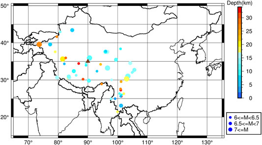
FIGURE 1. Spatial distribution of 56 M ≥ 6.0 earthquakes in the Chinese Mainland during 1998–2013. The triangle indicates the fixed location (35°N, 90°E) of GIM-TEC used in this paper.

Geomagnetic Dst and Solar Activity F_10.7 Index

Previous study suggested that the ionosphere was sensitive to solar and geomagnetic activities. Thus, it is necessary to analyze the geomagnetic indices and solar activity when identifying the earthquake-related TEC anomalies. The Dst index with a time resolution of 1-h provided by the World Data Center for Geomagnetism, Kyoto are used in this study. The geomagnetic storms can be classified into weak (−50 nT < Dst ≤ −30 nT), moderate (−100 nT < Dst ≤ −50 nT), and intense (Dst ≤ −100 nT) storms (Gonzalez et al., 1994). The solar radiation flux F_10.7 index provided by Space Physics Data Facility (SPDF) of NASA are used and F_10.7 is usually <100 SFU when solar activity is quiet (Guo et al., 2019).

Methods

We apply the SSA method to study and decompose the TEC time series and use Correlation value to analyze main components. SSA is a model-free approach to analyze the periodic oscillation of time series, which can be used to extract information from the original signal containing different periodic components (Keppenne and Ghil, 1992; Robert and Pascal, 1992). First, we obtain the TEC dataset for each earthquake 31 days before and after its occurrence day. The timespan of each dataset is 63 days and centers on the earthquake day. The SSA results will be different if using different data length. We use the length of 63 days to do SSA and use 60 days to analyze so that it is consistent with the previous results. Some researcher used the different data length to do analyze, depending on their own demand (Shi et al., 2020; Zhang et al., 2021). Next, we create a trajectory matrix with a window length of 20 days for each dataset. We choose 20 days because that the window length (L) of SSA should be 2 < L < N/2 (Golyandina et al., 2001) and we use N/3, where N is the length of the time series. Then we obtain the reconstructed time series after embedding, SVD, grouping, and diagonal averaging. For two reconstructed series X⁽¹⁾ and X⁽²⁾, the inner product is defined by (Golyandina et al., 2001).

where

To measure the degree of approximate separability between two series X⁽¹⁾ and X⁽²⁾, the Correlation value is defined as

The reconstructed components with large correlation values reflect that they are correlated from each other and usually composed of trend and periodic components, and the reconstructed components with small correlation values reflect that they are well separated from each other and contain different period components (Elsner, 2002). When extracting the reconstructed components, we select the first few principal components according to their energy, sorted by the corresponding eigenvalues λ_i. When the energy $\left(\frac{{\lambda }_i}{{{\displaystyle \sum }}_{i=1}^L{\lambda }_i}\right)$ of the i’th components is lower than 0.12%, we stop and take the rest components as the noises part. We select 0.12% as cut-off energy because this threshold value can ensure the TEC data of 56 earthquakes to exclude diurnal and semi-diurnal variations. Finally, we remove the semi-diurnal, diurnal, and long-term variations and obtain the residual denoted by ΔTEC. ΔTEC is mainly composed of computing errors and possible perturbations induced by earthquakes and geomagnetic activities. Note that here we use the TEC principal components for each earthquake 30 days before and after its occurrence day to avoid the boundary effects.

Results

Extraction of Main Components by SSA

We start by looking at an example of TEC data before and after the 2008 Wenchuan earthquake (Ms8.0) to show the extraction of main components by SSA. Figure 2 is an example of the Wenchuan earthquake from April 12, 2008 to June 11, 2008. We extract the first seven components based on the cut-off energy. Figure 2A is the correlation result of the first 20 reconstruction components by using SSA. It can be found the first seven components are separable and the eighth to later components are mixed with each other. Figure 2B shows the first seven reconstructed components. The first component is the trend component. The second to the fifth components are the diurnal variation and semi-diurnal variation, respectively. The sixth to the seventh components are approximately the 27-day variation and its half cycle.

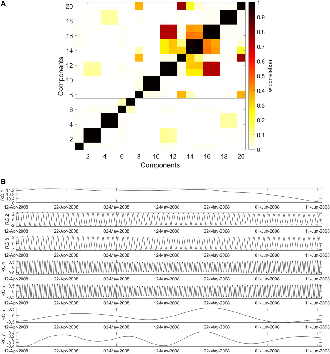
FIGURE 2. An example of GIM-TEC reconstructed data at fixed point (35°N, 90°E) 30 days before and after Wenchuan earthquake based on SSA (A) Correlation for the first 20 reconstructed components, and (B) the first seven reconstructed time series.

The ionosphere is an integrated product of the interaction between the Sun and the Earth’s environment. The TEC changes are mainly controlled by the intensities of solar electromagnetic radiation (He et al., 2012). Analyzing the correlation between the TEC component derived from SSA including trend and periodical components and geophysical indices including F_10.7 and Dst may help us to know the ionospheric effect from solar activity. The comparison of reconstructed components and F_10.7/Dst are as shown in Figure 3, and their Pearson correlation analysis are calculated. Because the F_10.7 data are of the 1-day resolution, the mean GIM-TEC of each day are used. The daily geomagnetic disturbance is measured by the minimum of the Dst indices on the day. As shown in Figure 3A, it is evident that the variation of the reconstructed components (RCs) 1–7 is similar to that of the F_10.7, and the RC 1 shows similar trend with F_10.7, suggesting a high correlation. The Pearson correlation analysis is demonstrated in Figure 3B, the correlation coefficient between RCs 1–7 and F_10.7 reaches 0.8, and the correlation coefficient between RC 1 and F_10.7 is 0.63. By the correlation analysis, it could be found that the influence from solar radiation at the daily timescale and above can be efficiently removed through the SSA method. In contrast, in Figure 3C, the correlation coefficient between RCs 1–7 and Dst is −0.22, between RC 1 and Dst is −0.26, showing a weak negative correlation.

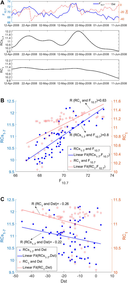
FIGURE 3. The correlation between reconstructed components and F_10.7/Dst of 30 days before and after the Wenchuan earthquake. (A) The solar activity time series F_10.7, Dst, the reconstructed components 1–7 and reconstructed component 1 of TEC data at the fixed point (35°N, 90°E) from April 12 to 11 June, (B) correlation of reconstructed components 1–7 and F_10.7 indices (in blue color), and correlation of reconstructed component 1 and F_10.7 indices (in red color), and (C) correlation of reconstructed components 1–7 and Dst indices (in blue color), and correlation of reconstructed component 1 and Dst indices (in red color).

After using SSA to extract the trend and periodic components which are mainly from the effects of solar activities, we subtract them from TEC data and obtain the residual ΔTEC. To give a more panoramic view, Figure 4A shows the original and reconstructed TEC results of the Wenchuan earthquake. Figure 4B shows the ΔTEC of the Wenchuan earthquake and its upper/lower bounds with ±RMS. The RMS is the root-mean-square error provided by the CODE on each grid point, which reflects the precision of the TEC data. Similar to (Guo et al., 2019), we use the RMS as the criterion for TEC anomaly detection. The ΔTEC value exceeding the upper/lower bounds implies that the ionosphere might be affected by solar activities or earthquakes. The ΔTEC at the fixed point (35°N, 90°E) for Wenchuan earthquake agrees with the results of (Chen et al., 2015). The ΔTEC decreased 1–4 days (from May 8 to May 12, 2008) before the earthquake and increased from May 3 to 5 May, as shown in Figure 4B.

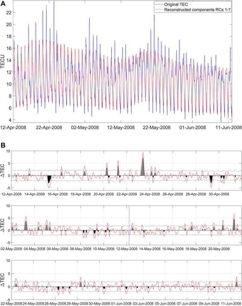
FIGURE 4. The ΔTEC time series of the point (35°N, 90°E) over a period of time for the 2008 Ms8.0 Wenchuan earthquakes (A)The contrast of original TEC and reconstructed by 1–7 components, (B) time series of ΔTEC and the upper or lower bounds. The red curve is the ΔTEC, denoted later by O. The two gray curves are the associated upper bound (UB) and lower bound (LB). The gray and black shaded areas denote differences of O-UB and LB-O, respectively.

Statistical Results

We select the most significant time 0600–1000 LT and calculate the percentages of the earthquakes with negative and positive anomalies that appear 30 days before and after the 56 earthquakes (following Chen et al., 2015). If one-third of the time in the 0600–1000 LT time span (3 h or more) occurred negative or positive anomalies, we count it a negative or positive anomaly day (following Chen et al., 2015). Figure 5 displays the percentages of the earthquakes with negative and positive precursory days and gives which kind of precursor is dominated. There are obvious negative anomalies 1–5 days before earthquakes, especially for M ≥ 6.8 and M ≥ 7.0. In general, the observed negative or positive precursors are consistent with the result of Chen et al. (2015). It should be noticed there are also higher positive abnormal proportion on 7–19 days before earthquakes, implying that the observed TEC tend to be relatively larger during this period. Therefore, if using the previous 15 days as the background, the upper and lower bounds of the dynamic ranges for TEC anomaly detection will become high. This might lead to more negative (below the lower bound) and less positive (above the upper bound) in the subsequent days. The proportion of anomalies overall in (Chen et al., 2015) is higher than that in our study, implying that the TEC anomalies reduce after applying SSA. This is consistent with the results of (He et al., 2012) that the ranges of TEC anomalies decreased on the global scale after removing background variations produced by solar radiations.

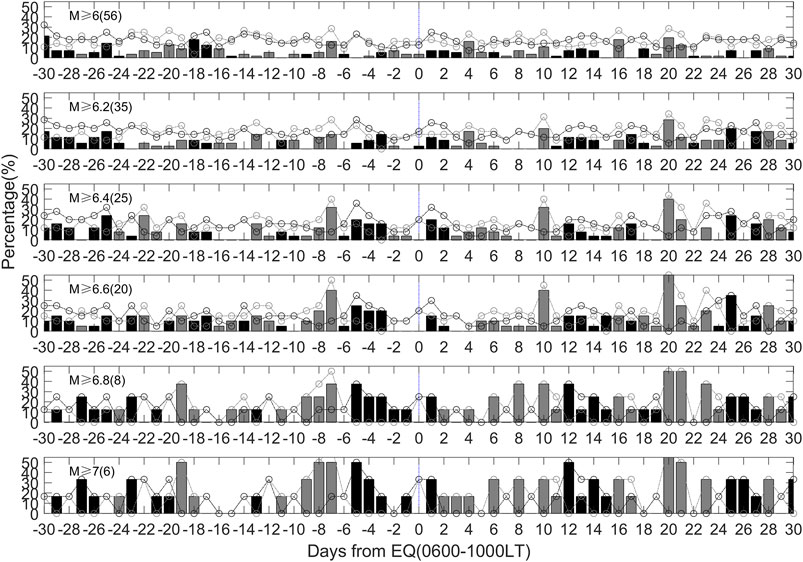
FIGURE 5. Percentages of the earthquakes with negative (black dot) and positive (gray dot) precursory days that appear 30 days before and after the earthquakes in China during 1998–2013 in the 0600–1000 LT. The black bar represents the amount of percentage in which negative anomaly is over positive anomaly, while the gray bar denotes the amount of percentage in which positive anomaly is over negative anomaly.

Even if the results in Figure 5 can be deemed to remove the influence of solar activity after SSA method, we redefine an anomaly hour when the TEC exceeds the upper or lower bound and both geomagnetic and solar activity are quiet (Dst index is more than −30 nT and F_10.7 is <100 SFU). If 3 h or more in the 0600–1000 LT occurred negative or positive anomalies, it is counted as a negative or positive anomaly day. Figure 6 shows results after ruling out the anomalies when geomagnetic or solar activities are not quiet. Negative anomalies are still dominant in 1–5 days before earthquakes, but the proportion decreased compared to that in Figure 5.

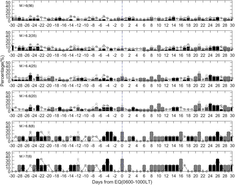
FIGURE 6. Percentages of the earthquakes with negative (black dot) and positive (gray dot) precursory days after ruling out the anomalies when geomagnetic or solar activities are not quiet. The black bar represents the amount of percentage in which negative anomaly is over positive anomaly, while the gray bar denotes the amount of percentage in which positive anomaly is over negative anomaly.

Discussion and Conclusions

A number of studies have shown the ionospheric TEC changes prior to great/mega earthquakes worldwide (e.g., Heki, 2011; Guo et al., 2015; He and Heki, 2016; Iwata and Umeno, 2016; He and Heki, 2017; Liu et al., 2018). As suggested by He et al. (2012), one of the key points is the elimination of ionospheric effect from solar radiation. In this study, we demonstrate another possible approach of SSA to eliminate such solar effects. By using SSA, the GIM-TEC anomalies prior to 56 M ≥ 6.0 earthquakes in the Chinese mainland during 1998–2013 have been revealed. Our findings agree with previous studies that negative anomalies are dominant during 1–5 days before earthquakes at the fixed point (Chen et al., 2015). The results persist after removing the data during intense geomagnetic and solar activity. As shown in both Figures 5 and 6, overall, the proportion of precursory days increases with the rise of earthquake magnitude, implying that the GIM-TEC anomalies are more likely to cooperate with stronger events.

Due to the ionospheric dynamic complexity, the earthquake-related perturbations might be far less than the seasonal and diurnal variations in the TEC data. Most studies took the previous 15/30 days as a reference and built the bounds for the TEC variation on the target day. As shown in Figure 2B, there are long-term trends in the TEC data. It may overestimate the background using the previous 15-day data if the TEC is on a downswing. On the contrary, the background may be underestimated if the TEC is in an uptrend. These may cause bias in detecting anomalies in the TEC data. As an attempt, we apply SSA to extract long-term, diurnal, and semi-diurnal variations. The residual ΔTEC contains errors, and possible perturbations induced by earthquakes and geomagnetic activities. By using the RMS as a threshold, we could remove the influences of computing errors to a certain degree, as the RMS gives the precision of the TEC data. The approach based on SSA and RMS have an advantage in identifying anomalous changes in TEC variation (Guo et al., 2019).

It should be noticed that some earthquakes’ epicenters may be far from the point at the GIM map that we used to analyze pre-seismic TEC variations, especially for the M6–M6.5 earthquakes, some of them are outside the Dobrovolsky earthquake preparation zone, leading to unobvious ionosphere reaction on the GIM selected point. Thus, we also take into account the pre-earthquake anomalies over the epicenter of the 56 earthquakes. Figure 7 shows the ΔTEC of the point which is closest to epicenter for the Wenchuan earthquake and its upper/lower bounds with ±RMS, here we use the same method above to extract the main components. There are more obvious positive and negative anomalies compared to Figure 4B, especially positive abnormal enhancement on May 9, which are in line with the results of Liu et al. (2009).

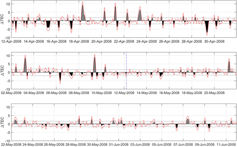
FIGURE 7. The ΔTEC time series of the point (30°N, 105°E) closest to the epicenter over a period of time for the 2008 Ms8.0 Wenchuan earthquakes.

In our statistical results, we focus on the time of 0600–1000 LT, if one-third of the time in the 0600–1000 LT (3 h or more) occurred negative or positive anomalies, we count it a negative or positive anomaly day (following Chen et al., 2015). For 1–5 days before M ≥ 6.0 earthquakes, the highest proportion of both positive and negative anomalies is about 23%, as shown in Figure 5. After ruling out the anomalies when intense geomagnetic or solar activities occur, the highest proportion of negative and positive anomalies are 19 and 13%, respectively, as seen in Figure 6. The proportion decreases compared to that in Figure 5 but negative anomalies are still dominant on 1–5 days before earthquakes. Figure 8 displays the percentages of the earthquakes with negative and positive precursory days over epicenter and gives which kind of precursor is dominated. In Figure 8, when using the TEC data close to the epicenter, the highest proportion of negative and positive anomalies increase to 28 and 34% on 1–5 days before M ≥ 6.0 earthquakes. The percentage is higher than those based on the TEC data in a fixed area in Figure 5, and the proportion increases with the magnitude. The proportions reach up to 100% (negative anomalies) and 33% (positive anomalies) for M ≥ 7.0 earthquakes. The results display that the anomalous variations are more significantly enhanced near the epicenter area. After ruling out the anomalies when intense geomagnetic or solar activities occur, the highest proportion of negative and positive anomalies are 15 and 18% respectively on 1–5 days before M ≥ 6.0 earthquakes, as shown in Figure 9, the proportion decreases compared to that in Figure 8 but negative anomalies are still dominant on 5 days before. The positive anomalies become obvious on 2–4 days before M ≥ 7.0 earthquakes, showing agreement with the positive abnormal enhancement on May 9, 3 days before the Wenchuan earthquake (Liu et al., 2009).

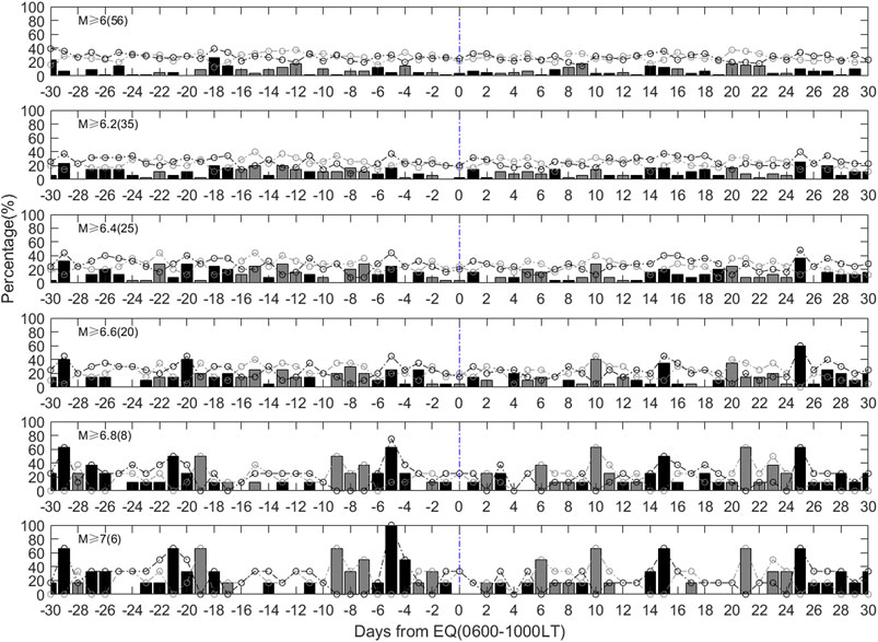
FIGURE 8. Percentages of the earthquakes with negative (black dot) and positive (gray dot) precursory days over epicenter that appear 30 days before and after the earthquakes in China during 1998–2013 in the 0600–1000 LT. The black bar represents the amount of percentage in which negative anomaly is over positive anomaly, while the gray bar denotes the amount of percentage in which positive anomaly is over negative anomaly.

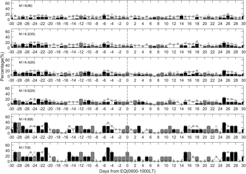
FIGURE 9. Percentages of the earthquakes with negative (black dot) and positive (gray dot) precursory days over epicenter after ruling out the anomalies when geomagnetic or solar activities are not quiet. The black bar represents the amount of percentage in which negative anomaly is over positive anomaly, while the gray bar denotes the amount of percentage in which positive anomaly is over negative anomaly.

The characteristics of pre-earthquake TEC changes were quite different in different areas. For example, the negative anomalies are found to be dominant 1–6 days before earthquakes in China (Liu et al., 2006; Chen et al., 2015); while the positive anomalies were considered prominent 1–5 days before earthquakes in Japan (Kon et al., 2011). If the earthquake samples are analyzed together, one may not find clear results as the correlation between either negative or positive anomalies and earthquakes will decrease. This might be the reason why no significant anomalies for global earthquakes were detected in some studies (Zhu and Jiang, 2020). In addition, the RMS of GIM-TEC data is different at different places due to the uneven distribution of GPS stations. The level of uncertainty is high if using the GIM-TEC with large RMS, so the data accuracy should be also considered when doing global statistical analysis.

As for the physical mechanism of ionospheric anomalies associated earthquake, there are several ideas have been proposed by some scholars in the previous studies. The internal gravity waves (IGWs) mechanism has been provided by Pertsev and Shalimov (1996), which origin from seismogenic zone with period of 1–3 h due to inflowing of lithosphere gases into the atmosphere before earthquake. Liu et al. (2016) indicated that the triggered acoustic and/or gravity waves in the atmosphere near the surface can be activated by vertical ground motions, which is considered coseismic phenomenon of Tohoku earthquake (Liu et al., 2016). Some scholars described the formation mechanism of earthquake ionospheric precursors by seismogenic electric field with amplitude (Sorokin and Chmyrev, 1999; Pulinets and Boyarchuk, 2004), which charged aerosols injected in the atmosphere and air ionization by radon followed by formation of large ion clusters of aerosol size during preparation. Namgaladze et al. (2009) proposed the most probable formation was the vertical transport of F2-region ionosphere plasma under action of zonal electric field (Namgaladze et al., 2009), some phenomena including geomagnetic conjugacy of the ionosphere precursors are the strong arguments in favor of this hypothesis. One more possible formation mechanism about the abnormal electro-magnetic fields and emissions has been offered (Hayakawa and Molchanov, 2002), which originated from the ground due to certain mechanisms such as piezo-electric effects (Finkelstein et al., 1973), tribo-electric effect (Gershenzon et al., 1993) and positive holes (P-holes) (Freund, 2000), although this mechanism is found to be insufficient because of the weak intensity of lithosphere radio emissions (Hayakawa, 2007). Among the possible mechanisms, air ionization by natural ground radioactivity is considered more credible by some scholars (Pulinets, 2012; Guo et al., 2015), which is conform to the ionospheric characteristics of Chile and Wenchuan earthquakes (Pulinets and Davidenko, 2014).

In summary, by applying the SSA method, we extract the trend and periodical background components of GIM-TEC to analyze the pre-earthquake ionospheric anomalies associated with M ≥ 6.0 earthquakes in the Chinese Mainland during 1998–2013. The results are consistent with those of Chen et al. (2015) in general. It is confirmed that the negative anomalies are dominant 1–5 days before the earthquake at the fixed point (35°N, 90°E) during 0600–1000 LT. The anomalies are more obvious near the epicenter area. As there are considerable errors in the GIM-TEC data, it is worthwhile to analyze high-precision satellite observation data to obtain more accurate results.

Data Availability Statement

Publicly available datasets were analyzed in this study. This data can be found here: “The TEC data are from the Center for Orbit Determination in Europe (ftp://ftp.unibe.ch/aiub/CODE), the solar radiation flux F_10.7 index are from Space Physics Data Facility (SPDF) of NASA (https://cdaweb.gsfc.nasa.gov/index.html/) and the Dst data are from the World Data Center for Geomagnetism (http://wdc.kugi.kyoto-u.ac.jp/).”

Author Contributions

Conceptualization, PH and HC; methodology, HC and PH; software, HC; validation, HC, MM, YC, QW, XS, KH, and PH; formal analysis, HC; investigation, HC, QW, XS, KH, and PH; resources, HC, MM, and YC; data curation, QW, XS, KH, and PH; writing—original draft preparation, HC; writing—review and editing, XS, KH, and PH; visualization, HC; supervision, PH; All authors have read and agreed to the published version of the manuscript.

Funding

This research is partly supported by National Natural Science Foundation of China (41974083, 41804049), China Seismic Experimental Site (2019CSES0105), and Grand-in-Aids for Scientific Research of Japan Society for Promotion of Science (26249060), and the Ministry of Education, Culture, Sports, Science, and Technology (MEXT) of Japan, under its observation and Research Program for Prediction of Earthquakes and Volcanic Eruptions.

Conflict of Interest

Author YC was employed by the company BGRIMM Technology Group. The remaining authors declare that the research was conducted in the absence of any commercial or financial relationships that could be construed as a potential conflict of interest.

Acknowledgments

We are very grateful to Orbit Determination in Europe (ftp://ftp.unibe.ch/aiub/CODE) for providing the GIM-TEC data. The solar radiation flux F_10.7 index were provided by Space Physics Data Facility (SPDF) of NASA (https://cdaweb.gsfc.nasa.gov/index.html/) and the Dst data were obtained from the World Data Center for Geomagnetism (http://wdc.kugi.kyoto-u.ac.jp/). We thank the reviewers for their useful comments and suggestions.

References

Afraimovich, E. L., and Astafyeva, E. I. (2008). TEC Anomalies-Local TEC Changes Prior to Earthquakes or TEC Response to Solar and Geomagnetic Activity Changes? Earth Planet. Sp. 60 (9), 961–966. doi:10.1186/bf03352851
Astafyeva, E., and Heki, K. (2011). Vertical TEC over Seismically Active Region during Low Solar Activity. J. Atmos. Solar-Terrestrial Phys. 73 (13), 1643–1652. doi:10.1016/j.jastp.2011.02.020
Carter, B. A., Kellerman, A. C., Kane, T. A., Dyson, P. L., Norman, R., and Zhang, K. (2013). Ionospheric Precursors to Large Earthquakes: A Case Study of the 2011 Japanese Tohoku Earthquake. J. Atmos. Solar-terrestrial Phys. 102, 290–297. doi:10.1016/j.jastp.2013.06.006
Chen, Y.-I., Huang, C.-S., and Liu, J.-Y. (2015). Statistical Evidences of Seismo-Ionospheric Precursors Applying Receiver Operating Characteristic (ROC) Curve on the GPS Total Electron Content in China. J. Asian Earth Sci. 114, 393–402. doi:10.1016/j.jseaes.2015.05.028
Dautermann, T., Calais, E., Haase, J., and Garrison, J. (2007). Investigation of Ionospheric Electron Content Variations before Earthquakes in Southern California, 2003–2004. J. Geophys. Res. Solid Earth 12 (B2), 121. doi:10.1029/2006jb004447
de Boor, C. (1978). A Practical Guide to Splines. Berlin: Springer-Verlag. doi:10.1007/978-1-4612-6333-3
Elsner, J. B. (2002). Analysis of Time Series Structure: SSA and Related Techniques. J. Am. Stat. Assoc. 97 (460), 1207–1208. doi:10.1198/jasa.2002.s239
Finkelstein, D., Hill, R. D., and Powell, J. R. (1973). The Piezoelectric Theory of Earthquake Lightning. J. Geophys. Res. (1896-1977). 78 (6), 992–993. doi:10.1029/JC078i006p00992
Freund, F. (2000). Time-resolved Study of Charge Generation and Propagation in Igneous Rocks. J. Geophys. Res. 105 (B5), 11001–11019. doi:10.1029/1999JB900423
Gershenzon, N. I., Gokhberg, M. B., and Yunga, S. L. (1993). On the Electromagnetic Field of an Earthquake Focus. Phys. Earth Planet. Interiors. 77 (1), 13–19. doi:10.1016/0031-9201(93)90030-D
Golyandina, N., Nekrutkin, V., and Zhigljavsky, A. (2001). Analysis of Time Series Structure. Monogr. Stat. Appl. Probab. 90, 144. doi:10.1201/9781420035841
Gonzalez, W. D., Joselyn, J. A., Kamide, Y., Kroehl, H. W., Rostoker, G., Tsurutani, B. T., et al. (1994). What Is a Geomagnetic Storm? J. Geophys. Res. 99 (A4), 5771. doi:10.1029/93ja02867
Guo, J., Li, W., Yu, H., Liu, Z., Zhao, C., and Kong, Q. (2015). Impending Ionospheric Anomaly Preceding the Iquique Mw8.2 Earthquake in Chile on 2014 April 1. Geophys. J. Int. 203 (3), 1461–1470. doi:10.1093/gji/ggv376
Guo, J., Shi, K., Liu, X., Sun, Y., Li, W., and Kong, Q. (2019). Singular Spectrum Analysis of Ionospheric Anomalies Preceding Great Earthquakes: Case Studies of Kaikoura and Fukushima Earthquakes. J. Geodynamics 124, 1–13. doi:10.1016/j.jog.2019.01.005
Han, P., Hattori, K., Zhuang, J., Chen, C.-H., Liu, J.-Y., and Yoshida, S. (2017). Evaluation of ULF Seismo-Magnetic Phenomena in Kakioka, Japan by Using Molchan's Error Diagram. Geophys. J. Int. 208 (1), 482–490. doi:10.1093/gji/ggw404
Han, P., Zhuang, J., Hattori, K., Chen, C.-H., Febriani, F., Chen, H., et al. (2020). Assessing the Potential Earthquake Precursory Information in ULF Magnetic Data Recorded in Kanto, Japan during 2000-2010: Distance and Magnitude Dependences. Entropy. 22 (8), 859. doi:10.3390/e22080859
Hattori, K., and Han, P. (2018). Statistical Analysis and Assessment of Ultralow Frequency Magnetic Signals in Japan as Potential Earthquake Precursors. Pre‐Earthquake Process. 14, 229–240. doi:10.1002/9781119156949.ch13
Hayakawa, M., and Molchanov, O. (2002). Seismo Electromagnetics Lithosphere–Atomosphere–Ionosphere Coupling. Tokyo, Japan: Terra Sci. Publ. Co.
Hayakawa, M. (2007). VLF/LF Radio Sounding of Ionospheric Perturbations Associated with Earthquakes. Sensors. 7, 1141–1158. doi:10.3390/s7071141
He, L., and Heki, K. (2017). Ionospheric Anomalies Immediately before M W 7.0-8.0 Earthquakes. J. Geophys. Res. Space Phys. 122 (8), 8659–8678. doi:10.1002/2017ja024012
He, L., and Heki, K. (2016). Three-dimensional Distribution of Ionospheric Anomalies Prior to Three Large Earthquakes in Chile. Geophys. Res. Lett. 43 (14), 7287–7293. doi:10.1002/2016gl069863
He, L., Wu, L., Pulinets, S., Liu, S., and Yang, F. (2012). A Nonlinear Background Removal Method for Seismo-Ionospheric Anomaly Analysis under a Complex Solar Activity Scenario: A Case Study of the M9.0 Tohoku Earthquake. Adv. Space Res. 50 (2), 211–220. doi:10.1016/j.asr.2012.04.001
He, Y., Yang, D., Qian, J., and Parrot, M. (2011). Response of the Ionospheric Electron Density to Different Types of Seismic Events. Nat. Hazards Earth Syst. Sci. 11, 2173–2180. doi:10.5194/nhess-11-2173-2011
Heki, K., and Enomoto, Y. (2015). M W Dependence of the Preseismic Ionospheric Electron Enhancements. J. Geophys. Res. Space Phys. 120 (8), 7006–7020. doi:10.1002/2015JA021353
Heki, K. (2011). Ionospheric Electron Enhancement Preceding the 2011 Tohoku-Oki Earthquake. Geophys. Res. Lett. 38 (17), 77. doi:10.1029/2011gl047908
Hirooka, S., Ichikawa, T., Hattori, K., Han, P., Yoshino, C., and Liu, J.-Y. (2016). Spatial and Temporal Distribution of the Pre-seismic Ionospheric Anomaly Prior to the 2011 off the Pacific Coast of Tohoku Earthquake (Mw9.0). IEEJ Trans. FM. 136, 265–271. doi:10.1541/ieejfms.136.265
Iwata, T., and Umeno, K. (2016). Correlation Analysis for Preseismic Total Electron Content Anomalies Around the 2011 Tohoku‐Oki Earthquake. J. Geophys. Res. Space Phys. 121 (9), 8969–8984. doi:10.1002/2016ja023036
Keppenne, C. L., and Ghil, M. (1992). Adaptive Filtering and Prediction of the Southern Oscillation index. J. Geophys. Res. 97 (D18), 20449–20454. doi:10.1029/92jd02219
Kon, S., Nishihashi, M., and Hattori, K. (2011). Ionospheric Anomalies Possibly Associated with M⩾6.0 Earthquakes in the Japan Area during 1998-2010: Case Studies and Statistical Study. J. Asian Earth Sci. 41 (4), 410–420. doi:10.1016/j.jseaes.2010.10.005
Lazaridou-Varotsos, M. S. (2013). The VAN Earthquake Prediction Method in Other Countries: Current Views. in Earthquake Prediction by Seismic Electric Signals: The success of the VAN Method over Thirty Years. (Berlin, Heidelberg: Springer), 191–202. doi:10.1007/978-3-642-24406-3_23
Le, H., Liu, J. Y., and Liu, L. (2011). A Statistical Analysis of Ionospheric Anomalies before 736M6.0+ Earthquakes during 2002-2010. J. Geophys. Res. Space Phys. 116, 49. doi:10.1029/2010ja015781
Li, M., and Parrot, M. (2013). Statistical Analysis of an Ionospheric Parameter as a Base for Earthquake Prediction. J. Geophys. Res. Space Phys. 118 (6), 3731–3739. doi:10.1002/jgra.50313
Li, Z. S., Wang, N. B., Li, M., Zhou, K., and Yuan, H. (2017). Evaluation and Analysis of the Global Ionospheric TEC Map in the Frame of International GNSS Services. Chin. J. Geophysics-Chinese Edition. 60 (10), 3718–3729.
Lin, J., Y, W., Y, Z. F., J, Q. X., and Y. Y, Z. (2009). Wenchuan Earthquake Ionosphere TEC Anomaly Detected by GPS. Chin. J. Geophysics-Chinese Edition 52 (1), 297–300. doi:10.1007/s10291-018-0759-1
Liu, J., Chen, C.-H., Sun, Y.-Y., Tsai, H.-F., Yen, H.-Y., Chum, J., et al. (2016). The Vertical Propagation of Disturbances Triggered by Seismic Waves of the 11 March 2011 M9.0 Tohoku Earthquake over Taiwan. Geophys. Res. Lett. 43, 37. doi:10.1002/2015gl067487
Liu, J., Hattori, K., and Chen, Y.-I. (2018). Application of Total Electron Content Derived from the Global Navigation Satellite System for Detecting Earthquake Precursors. Berlin: Springer, 305–317.
Liu, J. Y., Chen, Y. I., Chen, C. H., Liu, C. Y., Chen, C. Y., Nishihashi, M., et al. (2009). Seismoionospheric GPS Total Electron Content Anomalies Observed before the 12 May 2008Mw7.9 Wenchuan Earthquake. J. Geophys. Res. 114, 3–9. doi:10.1029/2008ja013698
Liu, J. Y., Chen, Y. I., Chuo, Y. J., and Chen, C. S. (2006). A Statistical Investigation of Preearthquake Ionospheric Anomaly. J. Geophys. Res. 111 (A5), 304. doi:10.1029/2005JA011333
Liu, J. Y., Chen, Y. I., Chuo, Y. J., and Tsai, H. F. (2001). Variations of Ionospheric Total Electron Content during the Chi‐Chi Earthquake. Geophys. Res. Lett. 28 (7), 151. doi:10.1029/2000gl012511
Liu, J. Y., Chuo, Y. J., Shan, S. J., Tsai, Y. B., Chen, Y. I., Pulinets, S. A., et al. (2004). Pre-earthquake Ionospheric Anomalies Registered by Continuous GPS TEC Measurements. Ann. Geophys. 22 (5), 1585–1593. doi:10.5194/angeo-22-1585-2004
Namgaladze, A. A., Klimenko, M. V., Klimenko, V. V., and Zakharenkova, I. E. (2009). Physical Mechanism and Mathematical Modeling of Earthquake Ionospheric Precursors Registered in Total Electron Content. Geomagn. Aeron. 49 (2), 252–262. doi:10.1134/S0016793209020169
Ouzounov, D., Pulinets, S., Hattori, K., and Taylor, P. (2018a). Pre-earthquake Processes: A Multidisciplinary Approach to Earthquake Prediction Studies. Hoboken: John Wiley & Sons.
Ouzounov, D., Pulinets, S., Liu, J., Hattori, K., and Han, P. (2018b). Multiparameter Assessment of Pre‐Earthquake Atmospheric Signals. Hoboken: John Wiley & Sons.
Pancheva, D., and Lastovicka, J. (1989). Solar or Meteorological Control of Lower Ionospheric Fluctuations (2-15 and 27 Days) in Middle Latitudes. Cambridge: Cambridge Uiversity Press.
Pancheva, D., Schminder, R., and Laštovička, J. (1991). 27-day Fluctuations in the Ionospheric D-Region. J. Atmos. Terrestrial Phys. 53, 1145–1150. doi:10.1016/0021-9169(91)90064-e
Parrot, M. (2012). Statistical Analysis of Automatically Detected Ion Density Variations Recorded by DEMETER and Their Relation to Seismic Activity. Ann. Geophys. 55 (1), 149–155. doi:10.1007/s11589-011-0813-3
Pertsev, N., and Shalimov, S. L. (1996). Generation of Atmospheric Gravitational Waves in a Seismo-Active Region and its Influence on the Ionosphere. Geomagn. Aeron. 36, 111–118.
Pisa, D., Němec, F., SantolíK, O., Parrot, M., and Rycroft, M. (2013). Additional Attenuation of Natural VLF Electromagnetic Waves Observed by the DEMETER Spacecraft Resulting from Preseismic Activity. J. Geophys. Res. Atmospheres 118 (8), 5286–5295. doi:10.1002/jgra.50469
Pulinets, S. A., Legen"Ka, A. D., Gaivoronskaya, T. V., and Depuev, V. K. (2003). Main Phenomenological Features of Ionospheric Precursors of strong Earthquakes. J. Atmos. Solar-Terrestrial Phys. 65 (16–18), 1337–1347. doi:10.1016/j.jastp.2003.07.011
Pulinets, S., and Davidenko, D. (2014). Ionospheric Precursors of Earthquakes and Global Electric Circuit. Adv. Space Res. 53 (5), 709–723. doi:10.1016/j.asr.2013.12.035
Pulinets, S. (2012). Low-Latitude Atmosphere-Ionosphere Effects Initiated by Strong Earthquakes Preparation Process. Int. J. Geophys. 12, 1–14. doi:10.1155/2012/131842
Robert, V., Pascal, Y., and Michael, G. (1992). Singular-spectrum Analysis: A Toolkit for Short, Noisy Chaotic Signals. Physica D Nonlinear Phenomena. 58, 95–126. doi:10.1016/0167-2789(92)90103-t
Rozhnoi, A., Solovieva, M., Parrot, M., Hayakawa, M.P.-F., and Biagi, (2015). VLF/LF Signal Studies of the Ionospheric Response to strong Seismic Activity in the Far Eastern Region Combining the DEMETER and Ground-Based Observations. Phys. Chem. Earth. Parts A/B/C. 85–86, 141–149. doi:10.1016/j.pce.2015.02.005
Sarkar, S., Tiwari, S., and Gwal, A. K. (2011). Electron Density Anomalies Associated with M≥5.9 Earthquakes in Indonesia during 2005 Observed by DEMETER. J. Atmos. Solar-Terrestrial Phys. 73 (16), 2289–2299. doi:10.1016/j.jastp.2011.06.004
Sarlis, N. V., Skordas, E. S., Christopoulos, S.-R. G., and Varotsos, P. A. (2020). Natural Time Analysis: The Area under the Receiver Operating Characteristic Curve of the Order Parameter Fluctuations Minima Preceding Major Earthquakes. Entropy. 22 (5), 583. doi:10.3390/e22050583
Sarlis, N. V., Skordas, E. S., Varotsos, P. A., Nagao, T., Kamogawa, M., Tanaka, H., et al. (2013). Minimum of the Order Parameter Fluctuations of Seismicity before Major Earthquakes in Japan. Proc. Natl. Acad. Sci. USA 110 (34), 13734–13738. doi:10.1073/pnas.1312740110
Saroso, S., Liu, J., Hattori, K., and Chen, C.-H. (2008). Ionospheric GPS TEC Anomalies and M ≧ 5.9 Earthquakes in Indonesia during 1993 - 2002. Terrestrial Atmos. Oceanic Sci. TERR ATMOS OCEAN SCI. 19, 481–488. doi:10.3319/TAO.2008.19.5.481(T)
Shah, M., Inyurt, S., Ehsan, M., Ahmed, A., Shakir, M., Ullah, S., et al. (2020). Seismo Ionospheric Anomalies in Turkey Associated with M ≥ 6.0 Earthquakes Detected by GPS Stations and GIM TEC. Adv. Space Res. 65 (11), 2540–2550. doi:10.1016/j.asr.2020.03.005
Shi, K., Guo, J., Liu, X., Liu, L., You, X., and Wang, F. (2020). Seismo-ionospheric Anomalies Associated with Mw 7.8 Nepal Earthquake on 2015 April 25 from CMONOC GPS Data. Geosci. J. 24 (4), 391–406. doi:10.1007/s12303-019-0038-3
Sorokin, V. M., and Chmyrev, V. (1999). Modification of the Ionosphere by Seismic Related Electric Field. Atmos. Ionospheric Electromagn. Phenomena Assoc. Earthq. 12, 805–818.
Tariq, M. A., Shah, M., Hernández-Pajares, M., and Iqbal, T. (2019). Pre-earthquake Ionospheric Anomalies before Three Major Earthquakes by GPS-TEC and GIM-TEC Data during 2015-2017. Adv. Space Res. 63 (7), 2088–2099. doi:10.1016/j.asr.2018.12.028
Thomas, J. N., Huard, J., and Masci, F. (2017). A Statistical Study of Global Ionospheric Map Total Electron Content Changes Prior to Occurrences of M ≥ 6.0 Earthquakes during 2000-2014. J. Geophys. Res. Space Phys. 122 (2), 2151–2161. doi:10.1002/2016ja023652
Xie, W., Hattori, K., and Han, P. (2019). Temporal Variation and Statistical Assessment of the B Value off the Pacific Coast of Tokachi, Hokkaido, Japan. Entropy. 21, 249. doi:10.3390/e21030249
Yao, Y., Chen, P., Wu, H., Zhang, S., and Peng, W. (2012). Analysis of Ionospheric Anomalies before the 2011 M W 9.0 Japan Earthquake. Chin. Sci. Bull. 57 (5), 500–510. doi:10.1007/s11434-011-4851-y
Zhang, X., Wang, Y., Boudjada, M., Liu, J., Magnes, W., Zhou, Y., et al. (2020). Multi-Experiment Observations of Ionospheric Disturbances as Precursory Effects of the Indonesian Ms6.9 Earthquake on August 05, 2018. Remote Sensing. 12 (24), 4050. doi:10.3390/rs12244050
Zhang, X., Zhao, S., Song, R., and Zhai, D. (2019). The Propagation Features of LF Radio Waves at Topside Ionosphere and Their Variations Possibly Related to Wenchuan Earthquake in 2008. Adv. Space Res. 63 (11), 3536–3544. doi:10.1016/j.asr.2019.02.008
Zhang, Y., Liu, X., Guo, J., Shi, K., Zhou, M., and Wang, F. (2021). Co-Seismic Ionospheric Disturbance with Alaska Strike-Slip Mw7.9 Earthquake on 23 January 2018 Monitored by GPS. Atmosphere. 12 (1), 83. doi:10.3390/atmos12010083
Keywords: total electronic content, earthquake, singular spectrum analysis, ionospheric anomaly, statistical analysis
Citation: Chen H, Miao M, Chang Y, Wang Q, Shen X, Hattori K and Han P (2021) Singular Spectrum Analysis of the Total Electron Content Changes Prior to M ≥ 6.0 Earthquakes in the Chinese Mainland During 1998–2013. Front. Earth Sci. 9:677163. doi: 10.3389/feart.2021.677163
Received: 07 March 2021; Accepted: 14 May 2021;
Published: 28 May 2021.
Edited by:
Juergen Pilz, University of Klagenfurt, AustriaReviewed by:
Xin Liu, Shandong University of Science and Technology, ChinaCopyright © 2021 Chen, Miao, Chang, Wang, Shen, Hattori and Han. This is an open-access article distributed under the terms of the Creative Commons Attribution License (CC BY). The use, distribution or reproduction in other forums is permitted, provided the original author(s) and the copyright owner(s) are credited and that the original publication in this journal is cited, in accordance with accepted academic practice. No use, distribution or reproduction is permitted which does not comply with these terms.
*Correspondence: Peng Han, hanp@sustech.edu.cn