Application of Bayesian Hyperparameter Optimized Random Forest and XGBoost Model for Landslide Susceptibility Mapping

Introduction

A landslide is defined as the movement of a mass of rock, earth, or debris down a slope (Cruden, 1991). Landslides are widely distributed around the world, especially in the areas with more active geological activities. They are one of the most destructive geohazards and cause catastrophic consequences. Landslides have brought significant loss to both the economy as well as people’s lives worldwide (Huang and Fan, 2013; Froude and Petley, 2018). Therefore, an effective solution that can reduce and mitigate the damage caused by landslide disasters needs to be urgently developed. Previous studies have shown that landslide susceptibility mapping (LSM) can reduce the risk of landslides and provide an essential basis and scientific support for decision-makers to deal with landslide disaster risk management and land use policies (Fell et al., 2008; Nourani et al., 2014).

In the past 30 years, with the rapid development of geographic information systems and computing technologies, various modeling methods of landslide spatial analysis and LSM have been proposed and widely used (Carrara et al., 2010; Reichenbach et al., 2018). The LSM methods can be divided into qualitative and quantitative evaluation methods (Aditian et al., 2018). The qualitative evaluation methods include landslide cataloging and is knowledge-driven based on the empirical evidence of experts to identify and analyze the geomorphology, topography, and geological conditions of a specific area, thus, being able to subjectively analyze the landslide susceptibility within the area (Kayastha et al., 2013; Myronidis et al., 2016). Therefore, the accuracy of the qualitative method primarily depends on the experience and knowledge of the experts and the quality and completeness of the collected landslide data. It is only suitable for small-scale LSM. On the other hand, the quantitative evaluation method establishes a statistical probability model based on mathematical knowledge to explore the relationship between landslides and influencing factors (Yilmaz, 2009; Tsangaratos et al., 2016). Commonly used quantitative methods such as frequency ratio (Huang et al., 2015; Li et al., 2016), the weight of evidence (Ilia and Tsangaratos, 2016), logistic regression (Ozdemir, 2011), and naive Bayes (Tsangaratos and Ilia, 2016), have been widely used in the LSM. In addition, machine learning has played an important role in LSM. Machine learning can handle the nonlinear relationship between the landslide effect factors (Marjanovic et al., 2011; Peethambaran et al., 2020; Wang et al., 2020). For instance, neural networks (Conforti et al., 2014; Polykretis and Chalkias, 2018), support vector machines (Xu et al., 2012; Sun et al., 2020), and decision trees (Nefeslioglu et al., 2010; Chen et al., 2018), these algorithms have strong robustness in overfitting and are suitable for nonlinear relationships between variables. Early studies were mainly based on a single model with limited accuracy and overfitting to predict susceptibility. In order to avoid these problems, an ensemble learning algorithm combining multiple decision trees is proposed. In particular, the algorithm can handle data sets with higher dimensions, more extensive data, as well as having stronger generalization capabilities (Lee et al., 2012; Kalantar et al., 2020). The ensemble learning algorithms include the random forest (RF), gradient decision tree, and extreme gradient boosting decision trees (XGBoost). Among them, RF and XGBoost have been studied by numerous scholars in LSM (Nguyen et al., 2017; Sevgen and Nefeslioglu, 2019; Sahin, 2020; Can et al., 2021). In order to verify the effects of the two in landslide susceptibility mapping RF, and XGBoost methods were used to map landslide susceptibility and compare the reliability and limitations of the two methods in this paper.

The model’s accuracy depends not only on the learning algorithm but also on the hyperparameters set before the model learning process. So, the purpose of optimizing the model is to improve the accuracy of the model further. Previous studies have used different models, model results to hyperparameter sensitivity, and different sampling strategies to study landslide susceptibility mapping (Yesilnacar and Topal, 2005; Nefeslioglu et al., 2008; Catani et al., 2013). However, only a few scholars optimized the model’s hyperparameters, such as the adaptive neuro-fuzzy inference system optimized by genetic algorithms (Chen et al., 2019). Sun et al. (2020a) developed an optimized RF method based on the hyperparameters optimization using Bayesian algorithms.

In this study, the main purpose is to: 1) use the Bayesian algorithm to optimize the hyperparameters of the RF, and XGBoost models in order to obtain the optimal model; 2) further discuss and compare the comprehensive performance of the two optimization models; 3) provide an effective mapping method for the susceptibility of loess landslides is proposed, and the research results can serve as disaster prevention, mitigation, and land use planning.

Study Area

Wuqi County is located in the northwestern part of the Loess District in Yan’an City, Shaanxi Province. The study area measures 3,791.5 km² and lies along longitudes 107°38′57″E to 108°32′49″E and latitudes 36°33′33″N to 37°24′27″N (Figure 1). The climate is a semi-arid temperate continental monsoon climate, with an average annual temperature of about 7.8°C. There is less precipitation in the region, with a dry climate and an average annual rainfall of approximately 483.4 mm. Wuqi County is located in the hinterland of the Loess Plateau, where precipitation is concentrated from July to September. The altitude of the Wuqi district is 1,199–1,772 m, and the elevation in the northwest is higher than in the southeast. The area is defined by having undulating beams, broken ground, rivers, ditches, and ravines throughout the county. The ground surface in the study area is covered by Quaternary Middle and Upper Pleistocene loess with a large accumulation thickness. The Pre-Quaternary strata are only exposed in deep-cut valleys and the lower part of the steep undulating beams slope; however, the occurrence is nearly horizontal. The exposed strata and lithology from old to new are as follows: Purple sandstone of the Huanhe-Huachi Formation (K_1h) of the Lower Cretaceous; Sandy clay of the Neogene Pliocene (N₂), and Quaternary (Q_p) eolian loess. Loess with well-developed vertical joints, fissures, and large pores, easily fail during times of precipitation (Wang et al., 2019). In addition, fine-grained materials in the loess, such as clay, soluble salts, and carbonates are quickly dissolved when exposed to water (Zhuang et al., 2020). As a result, landslides frequently occur under the effects of rainfall and engineering activity (Figure 2), which seriously threatens the safety of the local people’s lives and property. Therefore, it is crucial to evaluate the susceptibility of landslides in Wuqi County, which will help the local government to take necessary disaster prevention and mitigation measures.

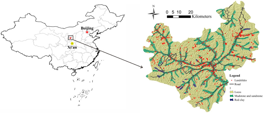
FIGURE 1. The study area and spatial distribution of the landslides.

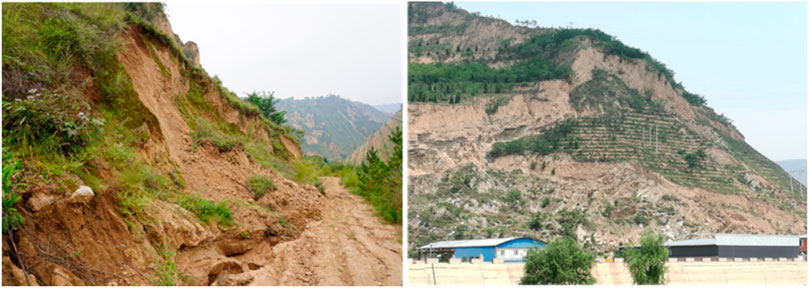
FIGURE 2. Field photos of two loess landslides.

Data Preparation

Data Usage

The susceptibility evaluation is based on the construction of the landslide spatial database. Through a large number of field surveys, geohazards data collection, and remote sensing image verification, the study area has identified 734 landslides. The distribution of the landslides is shown in Figure 1. Landslides can be divided into four types: landslides in the loess layer, landslides at the interface of loess-red clay, landslides at the interface of red clay-bedrock, and mudflow landslides in loess (Duan et al., 2011). The landslide scales are large, medium, and small according to the size of the slid body. The largest landslide volume is about 5.25 × 10⁵ m³, and the smallest is 8,200 m³. In addition, the major movement form of large-scale landslides is rotating landslide, while small and medium-sized landslides are translation and topples mainly. The data source is: 1) DEM data with a resolution of 12.5 m is used to extract terrain and landform related information such as altitude, slope, and topographic relief; 2) national 1:2.5 million geological maps are used to extract stratum lithology information; 3) vector maps of the national road network and water system network are used to extract road and water system distribution information; 4) Landsat8 images with a resolution of 30 m are used to extract vegetation coverage information on the ground; 5)the average annual rainfall of the country in the past 30 years; 6) field geological disaster survey data and Google Earth images are used to determine the spatial distribution of the landslides.

Prepare Landslide Influencing Factors

The development of landslides results from the combined effect of internal dynamic geological conditions and external environmental factors (Huang, 2007; Peng et al., 2019). Reichenbach et al. (2018) analyzed the research related to landslide susceptibility evaluation from 1983 to 2016. They found that 596 factors had been used for evaluations, and these factors could be classified into five types: geology, hydrology, landforms, land cover, and others. In this study, 14 landslide influence factors were selected for the landslide susceptibility model according to the geological environment conditions, landslide occurrence mechanism, and data availability of the study area, including altitude, slope, aspect, curvature, topographic relief, surface roughness, topographic wetness index (TWI), hypsometric integral (HI), lithology, normalized difference vegetation index (NDVI), average annual rainfall, distance to rivers, distance to roads, and distance to villages (Figure 3). Since the 14 factors are represented on different intervals or scales, all factors are converted into a grid with the DEM resolution (12.5 m × 12.5 m) for unification. Simultaneously, the continuous factors (altitude, slope, curvature, topographic relief, surface roughness, TWI, NDVI, annual average rainfall, and HI) are classified using the natural break point method. The remaining discrete factors are classified using the original natural grouping. The classification is shown in Table 1.

FIGURE 3. Landslide influencing factor maps. (A) Altitude, (B) Slope, (C) Aspect, (D) Curvature, (E) Topographic relief, (F) Surface roughness, (G) TWI, (H) HI, (I) Lithology, (J) Average annual rainfall, (K) Distance to rivers, (L) NDVI, (M) Distance to roads, (N) Distance to villages.

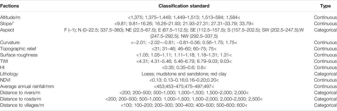
TABLE 1. Influencing factor categories of landslides.

The terrain factors include altitude, slope, aspect, curvature, topographic relief, surface roughness, TWI, and HI. The altitude affects potential energy and stress distribution in the slope during the development of a landslide, resulting in large potential energies leading to a landslide (Zaruba and Mencl, 2014). The slope directly determines the distribution of the slope stress, surface runoff, and groundwater recharge and has an important influence on the development of landslides (Varnes, 1984). The slope aspect determines the illumination time received by the slope surface. There are differences in surface humidity, vegetation coverage, and different slope aspects, which affect the distribution of pore water pressure and the physical and mechanical characteristics of rock and soil masses (Pourghasemi et al., 2012a). Curvature indicates the degree of distortion of a point on the slope surface, which has a certain impact on the confluence of surface water and the migration of landslides (Oh and Pradhan, 2011). Topographic relief is the difference between the maximum altitude and the minimum altitude within a 10 pixels radius, which describes the relief characteristics of the terrain surface (Bui et al., 2016). Surface roughness is a measure of the roughness and brokenness of the ground (Eq. 1) (Pradhan et al., 2010). TWI is defined as a function of the slope and the area contributed by the upstream unit width orthogonal to the direction of the water flow (Eq. 2). It quantifies the potential of the soil moisture content and potential runoff capacity at various points in the basin. The content and distribution of the soil’s moisture will affect the condition of the slopes rock mass, soil, and vegetation, thereby affecting the landslide (Pourghasemi et al., 2012b). HI reflects the degree of erosion of a watershed by collecting statistics on the altitude combination information of the watershed’s surface. It is a geological model that reflects the development stage of the watershed, an important indicator to reveal the morphology and development characteristics of the watershed, and a key factor affecting the erosion and slope evolution dynamics process (Singh et al., 2008).

where $A_S$is the specific catchment area (m²/m), $\text{β}$ is slope angle in degrees.

The geological factor is lithology and is the controlling factor for the development of landslides. Lithology is the material basis for the development of landslides. The lithology of different strata affects the probability, scale, and shape of landslides due to the hardness of the rock and the difference in rock mass structure. In previous studies, lithology has also been used to evaluate the susceptibility of landslides, especially in the loess areas (Chen et al., 2017a).

Environmental factors include the average annual rainfall, distance to rivers, and NDVI. Annual average rainfall refers to the average rainfall under a long-term duration, which affects the slope itself and the development of vegetation, surface runoff and other factors, thus affecting the development of landslides (Sun et al., 2020a). The distance to rivers is an important factor in inducing landslides. The wet saturated water of the river acting on the sliding area and part of the sliding body may reduce the shear strength of the soil and weaken the layers, thus, reducing the stability of the landslide (Hong et al., 2016). In addition, NDVI represents the degree of coverage of surface vegetation; the impact on landslides is reflected in the root consolidation of the vegetation roots on the slope; thus, slowing down the erosion and infiltration of the water flow (Ding et al., 2017).

The impact of human engineering activities on landslides is complex and involves many forms, such as the construction of roads and buildings, unreasonable impermeabilization and drainage outlets (Luti et al., 2020). When building roads, large-scale side slope excavation is required to change the natural shape and stress of the original slope toe. As a result, it is easy to form an empty surface, which has an unloading effect on the slope, thereby reducing the stability of the slope and leading to a landslide (Peng et al., 2014). The construction of buildings will also induce landslides, such as building houses, factories, mining, and other engineering activities, often requiring excavation of slopes and deep pits, damaging the surrounding mountains and reduce the overall stability above the slope (Sun et al., 2020b).

Methodology

In the present study, using Bayesian hyperparameters to optimize RF and XGBoost models for landslide susceptibility mapping, there are four main stages: 1) generating a list of landslides and landslide influencing factors; 2) training and validation data preparation, correlation analysis of impact factors; 3) using Bayesian hyperparameters to optimize the two models and susceptibility mapping; 4) validation and comparison of the two models (Figure 4).

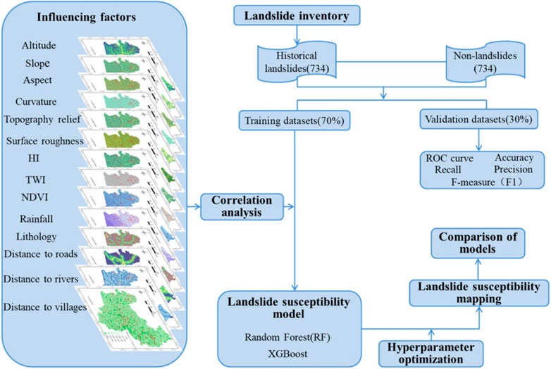
FIGURE 4. Flowchart of the research methodology used to provide the landslide susceptibility map.

Training and Validation Data Preparation

In the evaluation of landslide susceptibility, when advanced machine learning algorithms are used for modeling, a data set consisting of positive samples (landslides) and negative samples (non-landslides) is required to train and validate the model. In this paper, a single pixel in the center of each landslide area is selected as the landslide data (Atkinson and Massari, 1998). There are 734 landslides in the study area, divided into two parts, 70% (514) of the landslide data were randomly selected for training the model. In contrast, the remaining 30% (220) were used to validate the model. When selecting non-landslides, the landslide points were first buffered by 1 km to reduce the error, and 734 non-landslide points were randomly selected in the area outside the landslide point buffer zone. Similarly, the non-landslide points were randomly divided into two parts, one part was used for model training (70%, 514 non-landslides), and the other part was used for validating (30%, 220 non-landslides).

Correlation Analysis of Influencing Factors

In statistics, multicollinearity will occur when multiple variables are deeply linearly related in a multiple regression model, leading to inaccurate estimation of regression results (Bui et al., 2016). There are many methods to quantify multicollinearity, such as the Pearson correlation coefficient method (Ahlgren et al., 2014). The Pearson correlation coefficient can reflect the degree of linear correlation between two variables. Its value ranges from −1 to 1. −1 means that the two variables are completely negatively correlated, 1 means that the two variables are completely positively correlated, and 0 means that they are not correlated. In this study, the Pearson correlation coefficient was used to detect the correlation between the two influencing factors of landslides. If the value is greater than 0.5, it indicates a high correlation (Hong et al., 2020).

The Pearson correlation coefficient method was used for correlation analysis of 14 factors in the study area, and the results are shown in Figure 5. The figure shows that the correlation coefficients between slope and topographic relief are 0.61, and that between slope and surface roughness is 0.94, both of which are greater than 0.5, indicating a high correlation. Therefore, the topographic relief and surface roughness factors are excluded during the modeling of the landslide susceptibility, and the remaining 12 factors will be selected for landslide susceptibility evaluation.

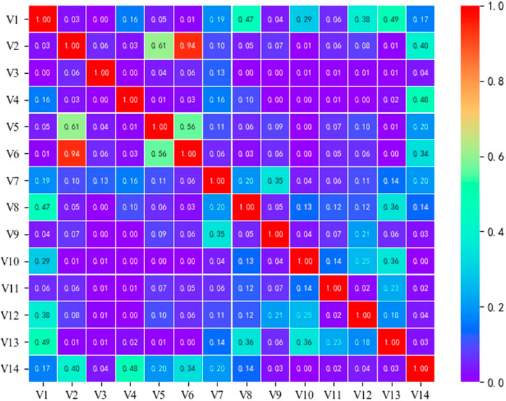
FIGURE 5. Pearson correlation coefficient results. V1 Altitude; V2 Slope; V3 Aspect; V4 Curvature; V5 Topographic relief; V6 Surface roughness; V7 HI; V8 NDVI; V9 Average annual rainfall; V10 Lithology; V11 Distance to roads; V12 Distance to rivers; V13 Distance to villages; V14 TWI.

Landslide Susceptibility Models

Random Forest

Random forest is one of the most practical algorithms in bagging ensemble strategies and was proposed by Breiman in 2001 (Breiman, 2001), which can be applied to classification, regression, and unsupervized learning. This algorithm has been widely used in many fields and shows excellent performance. Random forest is a combination classifier, which is composed of decision trees as the basic model. Each decision tree is trained with independent data sets; finally, the prediction result is obtained through voting or averaging. Random forest uses an autonomous bootstrap method for resampling. The method randomly extracts n (2/3 of the total sample) samples from the entire sample set with replacement to form a new training set. By training the new sample set, independent decision trees are built, and the trained n decision trees are combined into a forest. Each unextracted (1/3) sample is called out-of-bag data, which estimates the error inside each tree. It is used to evaluate the model performance to prevent over-fitting. The random forest model can rank the importance of various factors according to the Gini coefficient. The calculation formula of the Gini index is as follows:

Where G is the Gini index, which represents the probability that a randomly selected sample will be classified incorrectly in the sample set. ${\text{p}}_{\left(\text{s}\right)}$ is the probability of a sample being selected; ${\text{p}}_{\left(\text{m}\right)}$ is the probability of the sample being misclassified. The smaller the G, the smaller the probability that the selected sample in the set will be classified incorrectly, in other words, the higher the purity of the set. Conversely, the lower the purity of the set.

XGBoost

The XGBoost algorithm is an ensemble learning algorithm that integrates multiple decision tree models to form a bigger powerful classifier and is improved by gradient boosting decision trees (Chen and Guestrin, 2016). The core idea is to fit the residual of the previous prediction by learning a new function each time, thereby calculating the score corresponding to each node according to the sample characteristics. The sum of all the scores is the predicted value of the sample. which is

Where ${\text{y}}_{\text{i}}$ is the predicted value of the model, ${\text{x}}_{\text{i}}$ is the category label of the i sample, k is the number of trees, and ${\text{f}}_{\text{k}}$ is the k-th tree model. The XGBoot algorithm is used to learn k trees. When the loss function of the tree is the smallest, the model is the optimal model, and its prediction accuracy is also the highest, which can be expressed as

Where $\text{obj}\left(\text{t}\right)$ is the value of the loss function; $\text{l}\left({\text{y}}_{\text{i}},{\text{Y}}_{\text{i}}\right)$ is the training error; $\text{Ω}\left(\text{f}\left(\text{t}\right)\right)$ is the complexity of the entire tree; T is the total number of nodes in the leaves; γ is the division degree of the nodes to prevent overfitting; ω is the leaf node vector modulus; λ is the regularization coefficient. In the learning process, the objective function is used to characterize whether the algorithm at this time is optimal. XGBoost uses an algorithm to traverse the division points of all features. If the objective function after splitting is greater than that before splitting and exceeds the set threshold, it can be split. Stop splitting when the weight and maximum depth exceed the set threshold to prevent overfitting, and constantly find the appropriate learning function in the split. The condition function for judging the split is

Where $\frac{{\text{G}}_{\text{L}}^2}{{\text{H}}_{\text{L}}+\text{λ}}$ is the score of the left node after the node is cut; $\frac{{\text{G}}_{\text{L}}^2}{{\text{H}}_{\text{R}}+\text{λ}}$ is the score of the right node after the node is cut; $\frac{{\left({\text{G}}_{\text{L}}+{\text{G}}_{\text{R}}\right)}^2}{{\text{H}}_{\text{L}}+{\text{H}}_{\text{R}}+\text{λ}}$ is the score after cutting; ${\text{G}}_{\text{ain}}$ is the condition function for judging whether to split, if ${\text{G}}_{\text{ain}}$>0, then the split is performed, otherwise, the split is not performed.

Bayesian Optimization

The optimization of hyperparameters of machine learning algorithms is crucial in modeling and affects the model’s accuracy. However, the Bayesian optimization algorithm can quickly obtain the optimal value and is widely used to determine the optimal hyperparameter value of the model (Klein et al., 2016; Stuke et al., 2020). The Bayesian algorithm uses prior knowledge in the Gaussian process (GP) and has strong robustness. The algorithm only needs input and output data. It fits the posterior distribution of the objective function by increasing the number of samples, thereby realizing the hyperparameter optimization of the model and obtaining the optimal solution. First, assuming a collection function based on the prior distribution. Then, a new sampling point is used to test the objective function every time, using this information to update the prior distribution of the objective function. Finally, a check is performed on the global distribution given by the posterior distribution to find the most likely value. Usually, the probability model used for Bayes is GP because GP can easily calculate the predicted distribution of the target.

When GP is used as the basic model, assuming that the objective function f(x) being optimized is randomly sampled from GP, it can be expressed as f(x) ∼ GP(m(x),k (x,x’)), where k (x, x’) represents the covariance function, and m(x) represents the mean function. The intrinsic characteristics of the objective function f(x) (such as smoothness, additive noise, and amplitude) are specified by the covariance function k (x, x’), and the output result is the covariance of f(x) and f(x’). In the general Gaussian model, the probability of each feature needs to be calculated and then accumulated. In the multivariate Gaussian probability model, it is necessary to construct a covariance matrix and use the probability values of all eigenvectors. The GP model is as follows:

where μ (a mean), and cov (a covariance) are as follows:

Model Performance and Validation

In landslide susceptibility mapping, it is essential and necessary to validate the model’s performance (Wang et al., 2020). The receiver operating characteristic (ROC) curve is also a common method to test the accuracy of the evaluation of landslide susceptibility. The ROC curve is an indicator of continuous variables of data specificity and sensitivity (Bui et al., 2020). The area under the ROC curve (AUC) represents the accuracy of the model. When the AUC value is closer to 1, it indicates that the model’s prediction accuracy is higher. At the same time, the confusion matrix accuracy (ACC), recall, precision, and F-measure (F₁) are used to evaluate the predictive ability of the landslide model. The calculation is as follows:

Where TP (True Positive) and TN (True Negative) are the numbers of correctly classified landslides, FP (false positive) and FN (False negative) are the numbers of landslides incorrectly classified. For ACC, recall, precision, and F1, these values are between 0 and 1. With these values increasing, the model performance is better.

Results and Discussion

Bayesian Optimization RF Model

The RF model contains five hyperparameters, n_estimators, min_samples_split, max_depths, max_features, and bootstrap. n_estimators represent the number of decision trees; min_samples_split is the minimum number of samples to be split; max_depth is the maximum depth of the tree; max_features is the maximum number of features. The sample selection uses repeated sampling with replacement, so the bootstrap value is true. The Bayesian algorithm optimizes the remaining hyperparameters, and the hyperparameter value of each iteration is obtained. The mean square error (MSE) is selected to measure the model’s accuracy during hyperparameter optimization. As shown in Figure 6, the range of MSE under different hyperparameters is 0.259–0.361. After many hyperparameter optimization trainings in this study, the best parameters of the model (minimum MSE value) appeared before 30 iterations. After 30 iterations, the mean square error varied slightly, and the accuracy of the model could not improve anymore. Therefore, when performing hyperparameter optimization, the number of iteration times was choosenas 50, and the minimum MSE is 0.259 for the ninth iteration. The optimal hyperparameters are: [n_estimators:1,417, max_depths: 293, max_features: 6, min_samples_splits: 3].

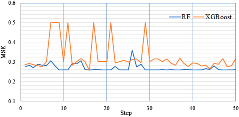
FIGURE 6. RF and XGBoost hyperparameter optimization (MSE).

Using the optimized hyperparameter values above 70% of the training samples, the RF is modeled and trained. The selected 12 factors are input into the optimized random forest model, and the landslide susceptibility index (LSI) of the study area is 0–1. It was divided into five levels using the natural break method (Figure 7A), which were respectively very low (0–0.215), low (0.215–0.372), middle (0.372–0.579), high (0.579–0.796), and very high (0.796–1). The area percentages of each susceptibility area class were 30.01, 24.59, 16.37, 15.05, and 13.99%, respectively. Figure 7A shows that the very high and high landslide susceptibility areas in Wuqi County are mainly distributed along rivers and valleys with severe soil erosion. The low susceptibility areas are mainly distributed in high altitude areas with less human engineering activities, which conform with the distribution of historical landslides.

FIGURE 7. Landslide susceptibility maps. (A) RF model, (B) XGBoost model.

Bayesian Optimization XGBoost Model

The XGBoost model contains five hyperparameters including, n_estimators, max_depths, learning_rate, gamma, and booster. Among them, n_estimators represent the number of decision trees; max_depths is the maximum depth of the tree; learning_rate is the shrinkage step used in the update process to prevent overfitting; gamma specifies the minimum loss function drop required for node splitting; booster indicates the booster parameters. The booster uses a tree-based model that is set to “gbtree.” The remaining hyperparameters are optimized via the Bayesian algorithm, and the hyperparameter value of each iteration is obtained. The XGBoost model performs hyperparameter optimization and 50 iterations. As shown in Figure 6, the MSE ranges from 0.256 to 0.499. At the 16th iteration, the MSE is minimal, and the model performs best. The hyperparameters are: [n_estimators: 668, max_depths: 3, learing_rate: 0.14, gamma: 0.1].

Using the optimized hyperparameter values above and 70% of the training samples, the XGBoost model is modeled and trained. The selected 12 factors are input into the optimized XGBoost model, and the LSI of the study area is 0–1. It was divided into five levels using the natural break method (Figure 7B), which were respectively very high (0.674–1), high (0.558–0.674), middle (0.455–0.558), low (0.372–0.455), and very low (0–0.372). The area percentages of each susceptibility area class were 13.90, 16.75, 23.55, 24.80, and 21%. Among them, the distribution results of very high and high prone areas are in good coherency with those predicted by the XGBoost model, which conforms with the distribution law of historical landslides.

Model Validation and Comparison

To evaluate the performance of the two models, the AUC value of the ROC curve was used to validate the training success power and prediction accuracy of the RF and the XGBoost model. The AUC of the training data set indicates the success ability of the model, and the validating data set represents the model’s predictive ability. As shown in Figure 8, the AUC values of the training data set of the RF and the XGBoost model are 0.98 and 0.97, respectively. The AUC values of the validating data set are 0.88 and 0.86. From the AUC values of the training data set, it can be seen that the models optimized by the two Bayesian algorithms show a good fit (success power). However, the success ability of the RF model training data is higher. Similarly, both optimized models have a higher predictive ability, while the RF model has a higher prediction accuracy. In addition, the ACC, recall, precision, and F-measure (F₁) of the confusion matrix are used to validate the validating data set of the two models. The results are shown in Table 2. All indicators show that the RF model and the XGBoost model optimized by the Bayesian algorithm show a better fit and higher prediction accuracy. However, from the overall indicators, the training and prediction of the RF model are better than the XGBoost model. Therefore, in the application of this research, the RF model optimized by the Bayesian algorithm has a higher predictive ability than the XGBoost model.

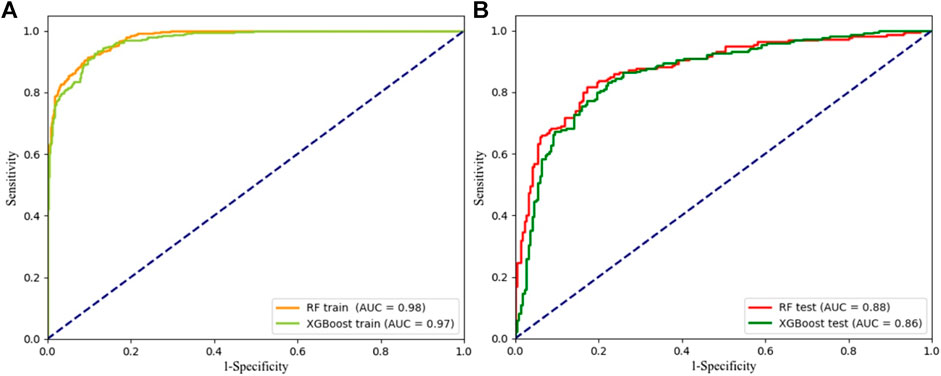
FIGURE 8. ROC curves of the RF and the XGBoost models. (A) the training data, (B) the validating data.

TABLE 2. Confusion matrix of the RF and the XGBoost models.

The two models were compared to the frequency ratio quantitative analysis based on the predicted landslide susceptibility zoning map and historical landslides. When the frequency ratio is greater than 1, the area is prone to landslides, and the higher the frequency ratio, the greater the possibility of landslides. Calculating the distribution of the landslides in each susceptibility grade, the frequency ratio was calculated (Table 3). The results show that the very high susceptibility of the RF model has 414 landslides, accounting for 56.40% of the total landslides. The very high susceptibility of the XGBoost model has 406 landslides, accounting for 55.31% of the total landslides. There are eight landslides in the very low susceptibility areas of the RF and the XGBoost model, accounting for 1.09% of the total landslides. However, the area of very low susceptibility (30.01%) of the RF model is larger than that of the XGBoost model (21.00%). The frequency ratio shows that the very high (4.03) and high (1.62) susceptibility areas of the RF model are larger than the very high (3.98) and high (1.59) frequency ratios of the XGBoost model; the very low (0.04) susceptibility area of the RF model is smaller than the very low (0.05) of the XGBoost model. The above statistical results show that the susceptibility evaluation results of the RF model and the distribution of landslides are more reasonable than the XGBoost model.

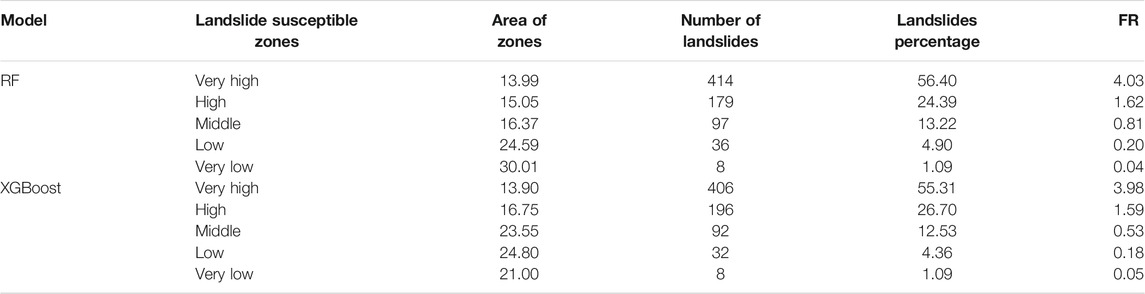
TABLE 3. Statistical results of the frequency ratio of the RF and the XGBoost models.

A common practice in landslide susceptibility studie is to compare (two or more) different models in terms of AUC, but the difference in the susceptibility map cannot be observed. Therefore, the method of Xiao et al. (2020) is used to compare the susceptibility map before and after optimization. Subtract the not optimazed susceptibility rate from the optimized one, and the two results are shown in Figure 9. The range of RF_BO-RF value is −0.544–0.668 (Figure 9A), the value of XGBoost_BO-XGBoost is −0.955–0.914 (Figure 9B), and the value of the map was broken at −0.20 and 0.20. Figure 9 compares the susceptibility maps of the two models before and after optimization. It can be observed that the difference of RF_BO-RF is small and there is no obvious distribution law, while the difference of XGBoost_BO-XGBoost is large. The overestimation (0.25–0.914) of XGBoost_BO-XGBoost is mainly distributed in the valley (low elevation areas), the underestimation (−0.955–−0.25) is distributed in ridges (high elevation areas). There are two reasons for the large difference between XGBoost_BO-XGBoost. On the one hand, it may be due to the over-fitting of the not optimized XGBoost model during training, which makes the error of the susceptibility map predicted by the not optimized model larger. Another reason may be that the factors of elevation and distance to rivers are related to the overestimation and underestimation of landslide susceptibility. In addition, we can also observe that RF is quite robust even without hyperoptimization, while XGBoost seems to have a higher need of optimization, as the not optimized version seems affected by relevant and systematic differences, driven by some thmatic layers.

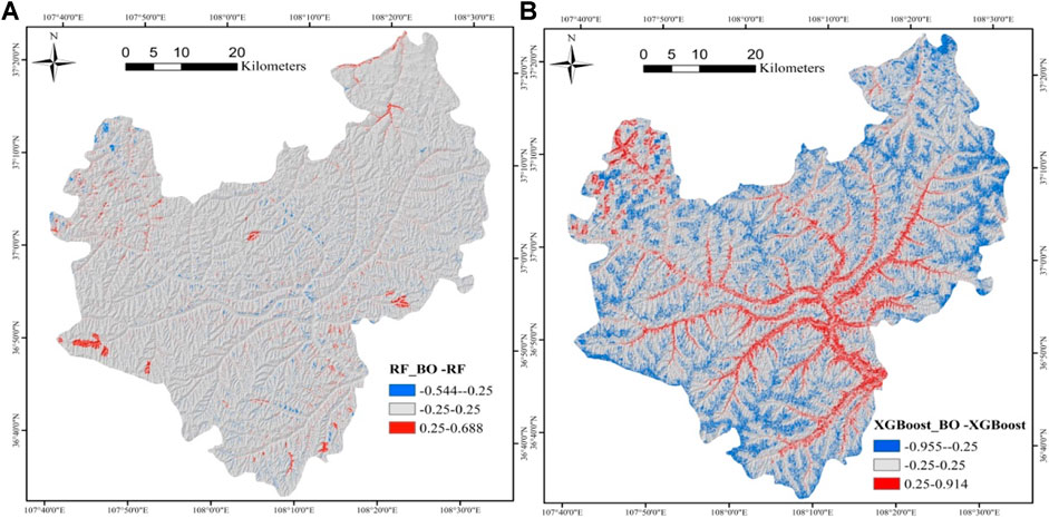
FIGURE 9. Two comparison maps. (A) RF_BO-RF, (B) XGBoost_BO-XGBoost.

Model Optimization

The hyperparameters of machine learning algorithms impact model accuracy (Rong et al., 2020; Sam et al., 2020); however, in previous studies, the determination of better performing hyperparameters is more often selected by trial-and-error methods and grid search (Chen et al., 2017b; Pham et al., 2019). This method may miss the best parameters, consume much time, and significantly reduce accuracy and efficiency. For this reason, to quickly find the best hyperparameters, the Bayesian optimization algorithm can make up for the shortcomings of low accuracy and efficiency by obtaining the best hyperparameters of the model. The algorithm fits the posterior distribution of the objective function by increasing the number of samples, input, and output data, to realize the hyperparameter optimization of the model and obtain the best parameters. The results before and after the hyperparameter optimization of the RF model and the XGBoost model are shown in Figure 10. Both the AUC of the RF model training data before and after optimization was 0.98, and the AUC of the validating data before and after optimizing by Bayesian algorithm are 0.84 and 0.88. The AUC of the training data before the XGBoost model is optimized is 1.0, and the validating data is 0.83. The AUC of the training and validating data after Bayesian algorithm optimization (XGBoost_BO) are 0.97 and 0.86, respectively. The results of the above two optimization models show that the model optimized by the Bayesian algorithm has a good fit on training, and the prediction accuracy has also been improved. Meanwhile, from the AUC of the training data before and after optimizing the XGBoost model, it can be observed that the optimization of the hyperparameters can prevent the overfitting problem. Therefore, the model’s fit and prediction performance can be increased to a certain extent. As a result, the results of the landslide susceptibility evaluation are more accurate and reliable using the Bayesian algorithm to optimize the hyperparameters.

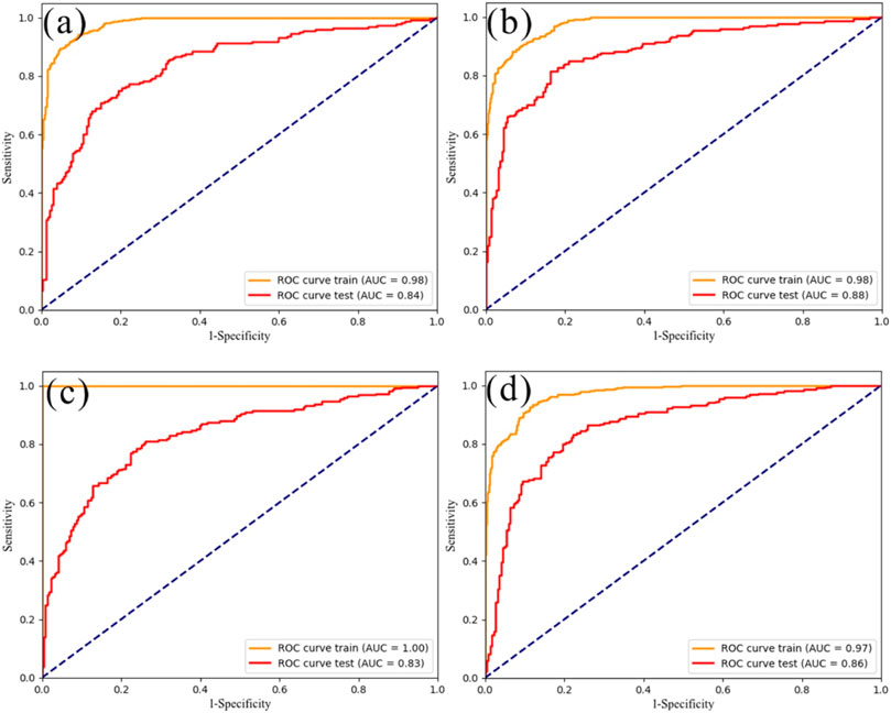
FIGURE 10. ROC curves. the RF models (A) before and (B) after hyperparameter optimization; the XGBoost models (C) before and (D) after hyperparameter optimization.

Besides the model’s own parameters that affect the accuracy of the model, there are also landslide sampling strategies. There are many sampling methods for landslide presence data, for example, Seed cell, Scarp, Point, and fuzzy C-means clustering (Che et al., 2012; Alimohammadlou et al., 2014). They have been successfully applied to landslide susceptibility mapping. Yilmaz (2010) compared the influence of scarp, seed cell and point sampling strategy on landslide susceptibility mapping, and the results showed that the Scarp sampling strategy gave the best results than the point, whereas the scarp and seed cell methods can be evaluated relatively similar. Dou et al. (2020) compared the predictive capabilities of four types of samples were extracted from the polygon shapes, i.e., samples of landslide scarp, centroid of scarp, samples of landslide body and centroid of body, respectively. The order of predictive power is in the following order: landslide scarp > landslide body > centroid of scarp > centroid of the body. Therefore, the landslide sampling strategy also has a greater impact on the predictive ability of the model. In the future research, not only the influence of the model parameters, but also the influence of the landslide sampling strategy should be considered. In addition, the number of landslide samples will also affect the evaluation results of susceptibility. Sufficient landslide samples can make the trained model more stable and the predicted results more accurate. In this study, the landslide data used comes from geological hazard surveys in the field, geohazards data collection and remote sensing image verification. In this process, recent individual landslide disaster data may be missed, making the list of landslides not very complete. Therefore, interferometric synthetic aperture radar (InSAR) technology can be used to identify recent landslides in future research (Zhao et al., 2019), to make up for the shortcomings of difficulty in collecting recent landslide data, and to make the evaluation results more reliable.

Importance of Influencing Factor

The occurrence of landslides is controlled by multiple influencing factors as well as the differences in how each factor affects the occurrence (Wu et al., 2020). Therefore, it is necessary to study the importance and mechanism of each influencing factor, which can provide guidance for predicting and preventing landslide disasters. In this study, the RF model with high prediction performance was used to analyze the importance of the influencing factors. Based on the “Gini coefficient” of the RF model, the contribution of the 12 factors in the study area to the occurrence of landslides was obtained. As shown in Figure 11, the importance of the 12 factors in descending order are altitude (0.229), lithology (0.178), average annual rainfall (0.134), distance to rivers (0.122), HI (0.059), slope (0.057), TWI (0.052), NDVI (0.051), distance to roads (0.045), aspect (0.030), distance to villages (0.023), and curvature (0.020).

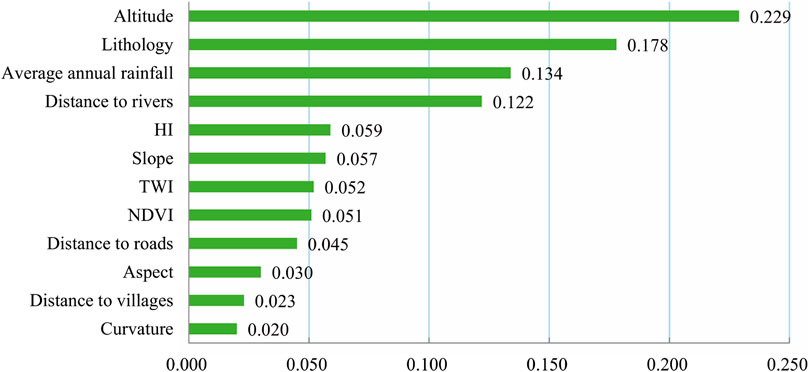
FIGURE 11. Importance of influencing factors based on the RF model.

The importance of the influencing factors obtained from the RF model found that altitude, lithology, average annual rainfall, and distance to rivers are important factors affecting the occurrence of landslides in the study area. According to the distribution of landslides in different altitude ranges, the frequency ratio map (Figure 12A) is obtained. The frequency ratio at the altitude of 1,199–1,375 m is highest at 2.91, and the frequency ratio gradually decreases with an increase in altitude. In addition, 65% of landslides occur in areas where the altitude is less than 1,449 m. Human engineering activities are intense in low altitude areas, vegetation coverage is small, slopes are severely disturbed, and landslide disasters occur frequently. Relatively the high-altitude area has fewer human engineering activities and fewer landslides. The results of the analysis of the influence of rivers on landslides are shown in Figure 12B. There are 361 landslides within 200 m from the river, the frequency ratio which is up to 2.45. In addition, the frequency ratio gradually decreases as the distance from the river increases. At the same time, 83% of landslides occur within 500 m from the river. This is due to long-term running water where both riverbanks have been severely eroded and scoured. As a result, the natural stress and shape of the slope have been destroyed, and slopes are liable to instability. The landslides in the study area are mainly loess and loess-bedrock dual structure landslides. However, many research results show that rainfall is the leading reason forloess landslides and plays a decisive role in loess landslides (Wang et al., 2014; Peng et al., 2015). A large amount of rainfall will soften the soil and affect the surface runoff to cause the erosion of the slope surface, reduce the stability of the slope, and make the slope prone to instability. Therefore, rainfall plays an essential role in the occurrence of landslides in Wuqi County, which is consistent with the importance of the RF model's influencing factors.

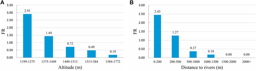
FIGURE 12. Frequency ratio chart of altitude and distance to rivers. (A) altitude, (B) distance to rivers.

Conclusion

In this study, the Bayesian hyperparameter optimization RF and XGBoost models were used for landslide susceptibility mapping. Wuqi County, where landslide disasters are relatively frequent, is where the research was conducted. Both optimized hyperparameter models were evaluated and compared, and the importance of the landslide influence factors was analyzed and concluded as follow:

1) The validating data AUC of the RF and the XGBoost models optimized based on the Bayesian hyperparameter optimization are 0.88 and 0.86, respectively, which are 4 and 3% higher than before. The training data shows a high degree of fit. Therefore, the use of the Bayesian algorithm to optimize hyperparameters can improve the fit of the two models and the performance of prediction to a certain extent;

2) In this study area, both optimized models have higher accuracy for landslide susceptibility mapping. However, the RF model has a better fit and a higher predictive ability than the XGBoost model.

3) According to the analysis of the landslide influencing factors in the study area, it was found that altitude, lithology, average annual rainfall, and distance to rivers are the main influencing factors that affect the occurrence of landslides.

Data Availability Statement

The original contributions presented in the study are included in the article/Supplementary Material, further inquiries can be directed to the corresponding author.

Author Contributions

JZhu initiated and sponsored this work; SW carried out the susceptibility analysis and wrote the manuscript; JZhe, HF, JK, and JZha assisted with data analysis. All authors contributed to the redaction and final revision of the manuscript.

Funding

This study was financially supported by the National Natural Science Foundation of China: 42090053, 41922054 and Fundamental Research Funds for the Central Universities, CHD 300102260302.

Conflict of Interest

The authors declare that the research was conducted in the absence of any commercial or financial relationships that could be construed as a potential conflict of interest.

References

Aditian, A., Kubota, T., and Shinohara, Y. (2018). Comparison of Gis-Based Landslide Susceptibility Models Using Frequency Ratio, Logistic Regression, and Artificial Neural Network in a Tertiary Region of Ambon, indonesia. Geomorphology. 318, 101–111. doi:10.1016/j.geomorph.2018.06.006
Ahlgren, P., Jarneving, B., and Rousseau, R. (2003). Requirements for a Cocitation Similarity Measure, with Special Reference to pearson's Correlation Coefficient. J. Am. Soc. Inf. Sci. 54 (6), 550–560. doi:10.1002/asi.10242
Alimohammadlou, Y., Najafi, A., and Gokceoglu, C. (2014). Estimation of Rainfall-Induced Landslides Using ANN and Fuzzy Clustering Methods: a Case Study in Saeen Slope, Azerbaijan Province, Iran. CATENA. 120, 149–162. doi:10.1016/j.catena.2014.04.009
Atkinson, P. M., and Massari, R. (1998). Generalised Linear Modelling of Susceptibility to Landsliding in the central Apennines, italy. Comput. Geosciences. 24 (4), 373–385. doi:10.1016/S0098-3004(97)00117-9
Bui, D. T., Tran, A. T., Klempe, H., Pradhan, B., and Revhaug, I. (2016). Spatial Prediction Models for Shallow Landslide Hazards: a Comparative Assessment of the Efficacy of Support Vector Machines, Artificial Neural Networks, Kernel Logistic Regression, and Logistic Model Tree. Landslides. 13 (2), 361–378. doi:10.1007/s10346-015-0557-6
Bui, D. T., Tsangaratos, P., Nguyen, V.-T., Liem, N. V., and Trinh, P. T. (2020). Comparing the Prediction Performance of a Deep Learning Neural Network Model with Conventional Machine Learning Models in Landslide Susceptibility Assessment. Catena. 188 (2020), 104426. doi:10.1016/j.catena.2019.104426
Can, R., Kocaman, S., and Gokceoglu, C. (2021). A Comprehensive Assessment of XGBoost Algorithm for Landslide Susceptibility Mapping in the Upper Basin of Ataturk Dam, Turkey. Appl. Sci., 11, 4993. doi:10.3390/app11114993
Carrara, A., Cardinali, M., Detti, R., Guzzetti, F., Pasqui, V., and Reichenbach, P. (1991). Gis Techniques and Statistical Models in Evaluating Landslide hazard. Earth Surf. Process. Landforms. 16 (5), 427–445. doi:10.1002/esp.3290160505
Catani, F., Lagomarsino, D., Segoni, S., and Tofani, V. (2013). Landslide Susceptibility Estimation by Random Forests Technique: Sensitivity and Scaling Issues. Nat. Hazards Earth Syst. Sci. 13 (11), 2815–2831. doi:10.5194/nhess-13-2815-2013
Che, V. B., Kervyn, M., Suh, C. E., Fontijn, K., Ernst, G. G. J., del Marmol, M.-A., et al. (2012). Landslide Susceptibility Assessment in Limbe (Sw cameroon): a Field Calibrated Seed Cell and Information Value Method. Catena. 92 (none), 83–98. doi:10.1016/j.catena.2011.11.014
Chen, T., and Guestrin, C. (2016). “XGBoost: A Scalable Tree Boosting System.” In Proceedings of the 22nd ACM SIGKDD International Conference on Knowledge Discovery and Data Mining (KDD '16). New York, NY, USA: Association for Computing Machinery, 785–794. doi:10.1145/2939672.2939785
Chen, W., Panahi, M., Tsangaratos, P., Shahabi, H., Ilia, I., Panahi, S., et al. (2019). Applying Population-Based Evolutionary Algorithms and a Neuro-Fuzzy System for Modeling Landslide Susceptibility. Catena. 172, 212–231. doi:10.1016/j.catena.2018.08.025
Chen, W., Pourghasemi, H. R., Panahi, M., Kornejady, A., Wang, J., Xie, X., et al. (2017a). Spatial Prediction of Landslide Susceptibility Using an Adaptive Neuro-Fuzzy Inference System Combined with Frequency Ratio, Generalized Additive Model, and Support Vector Machine Techniques. Geomorphology. 297, 69–85. doi:10.1016/j.geomorph.2017.09.007
Chen, W., Xie, X., Wang, J., Pradhan, B., Hong, H., Bui, D. T., et al. (2017b). A Comparative Study of Logistic Model Tree, Random forest, and Classification and Regression Tree Models for Spatial Prediction of Landslide Susceptibility. Catena. 151 (1), 147–160. doi:10.1016/j.catena.2016.11.032
Chen, W., Zhang, S., Li, R., and Shahabi, H. (2018). Performance Evaluation of the GIS-Based Data Mining Techniques of Best-First Decision Tree, Random forest, and Naïve Bayes Tree for Landslide Susceptibility Modeling. Sci. Total Environ. 644 (dec.10), 1006–1018. doi:10.1016/j.scitotenv.2018.06.389
Conforti, M., Pascale, S., Robustelli, G., and Sdao, F. (2014). Evaluation of Prediction Capability of the Artificial Neural Networks for Mapping Landslide Susceptibility in the Turbolo River Catchment (Northern Calabria, italy). Catena. 113, 236–250. doi:10.1016/j.catena.2013.08.006
Cruden, D. M. (1991). A Simple Definition of a Landslide. Bull. Int. Assoc. Eng. Geology. 43, 27–29. doi:10.1007/BF02590167
Ding, Q., Chen, W., and Hong, H. (2017). Application of Frequency Ratio, Weights of Evidence and Evidential Belief Function Models in Landslide Susceptibility Mapping. Geocarto Int. 32 (6), 1–21. doi:10.1080/10106049.2016.1165294
Dou, J., Yunus, A. P., Merghadi, A., Shirzadi, A., Nguyen, H., Hussain, Y., et al. (2020). Different Sampling Strategies for Predicting Landslide Susceptibilities Are Deemed Less Consequential with Deep Learning. Sci. Total Environ. 720, 137320. doi:10.1016/j.scitotenv.2020.137320
Duan, J., Zhao, F., and Chen, X. (2011). Types and Spatio-Temporal Distribution of Loess Landslides in Loess Plateau Region—A Case Study in Wuqi County. J. Catastrophology. 26 (04), 52–56. doi:10.1007/s12583-011-0163-z
Fell, R., Corominas, J., Bonnard, C., Cascini, L., Leroi, E., and Savage, W. Z. (2008). Guidelines for Landslide Susceptibility, hazard and Risk Zoning for Land Use Planning. Eng. Geology. 102 (3-4), 85–98. doi:10.1016/j.enggeo.2008.03.022
Froude, M. J., and Petley, D. N. (2018). Global Fatal Landslide Occurrence from 2004 to 2016. Nat. Hazards Earth Syst. Sci. 18 (8), 2161–2181. doi:10.5194/nhess-18-2161-2018
Hong, H., Liu, J., and Zhu, A.-X. (2020). Modeling Landslide Susceptibility Using LogitBoost Alternating Decision Trees and forest by Penalizing Attributes with the Bagging Ensemble. Sci. Total Environ. 718, 137231. doi:10.1016/j.scitotenv.2020.137231
Hong, H., Pourghasemi, H. R., and Pourtaghi, Z. S. (2016). Landslide Susceptibility Assessment in Lianhua County (china): a Comparison between a Random forest Data Mining Technique and Bivariate and Multivariate Statistical Models. Geomorphology. 259 (Apr.15), 105–118. doi:10.1016/j.geomorph.2016.02.012
Huang, J., Zhou, Q., and Wang, F. (2015). Mapping the Landslide Susceptibility in Lantau Island, hong kong, by Frequency Ratio and Logistic Regression Model. Ann. Gis. 21 (3), 191–208. doi:10.1080/19475683.2014.992373
Huang, R., and Fan, X. (2013). The Landslide story. Nat. Geosci. 6 (5), 325–326. doi:10.1038/ngeo1806
Huang, R. (2007). Large-scale Landslides and Their Sliding Mechanisms in china since the 20th century. Chin. J. Rock Mech. Eng. 26 (3), 433–454.
Ilia, I., and Tsangaratos, P. (2016). Applying Weight of Evidence Method and Sensitivity Analysis to Produce a Landslide Susceptibility Map. Landslides. 13 (2), 379–397. doi:10.1007/s10346-015-0576-3
Kalantar, B., Ueda, N., Saeidi, V., Ahmadi, K., Halin, A. A., and Shabani, F. (2020). Landslide Susceptibility Mapping: Machine and Ensemble Learning Based on Remote Sensing Big Data. Remote Sensing. 12, 1737. doi:10.3390/rs12111737
Kayastha, P., Dhital, M. R., and De Smedt, F. (2013). Evaluation and Comparison of Gis Based Landslide Susceptibility Mapping Procedures in Kulekhani Watershed, nepal. J. Geol. Soc. India. 81 (2), 219–231. doi:10.1007/s12594-013-0025-7
Klein, A., Falkner, S., Bartels, S., Hennig, P., and Hutter, F. (2016). Fast Bayesian Optimization of Machine Learning Hyperparameters on Large Datasets. Neural Netw. 106, 294–302. doi:10.1093/obo/9780195389661-0226
Lee, M.-J., Choi, J.-W., Oh, H.-J., Won, J.-S., Park, I., and Lee, S. (2012). Ensemble-based Landslide Susceptibility Maps in Jinbu Area, Korea. Environ. Earth Sci. 67, 23–37. doi:10.1007/s12665-011-1477-y
Li, L., Lan, H., Guo, C., Zhang, Y., Li, Q., and Wu, Y. (2016). A Modified Frequency Ratio Method for Landslide Susceptibility Assessment. Landslides. 14, 727–741. doi:10.1007/s10346-016-0771-x
Luti, T., Segoni, S., Catani, F., Munafò, M., and Casagli, N. (2020). Integration of Remotely Sensed Soil Sealing Data in Landslide Susceptibility Mapping. Remote Sensing. 12 (9), 1486. doi:10.3390/rs12091486
Marjanovic, M., Kovacevic, M., Bajat, B., and Voženílek, V. (2011). Landslide Susceptibility Assessment Using Svm Machine Learning Algorithm. Eng. Geology. 123 (3), 225–234. doi:10.1016/j.enggeo.2011.09.006
Myronidis, D., Papageorgiou, C., and Theophanous, S. (2016). Landslide Susceptibility Mapping Based on Landslide History and Analytic Hierarchy Process (AHP). Nat. Hazards. 81 (1), 245–263. doi:10.1007/s11069-015-2075-1
Nefeslioglu, H. A., Gokceoglu, C., and Sonmez, H. (2008). An Assessment on the Use of Logistic Regression and Artificial Neural Networks with Different Sampling Strategies for the Preparation of Landslide Susceptibility Maps. Eng. Geology. 97 (3-4), 171–191. doi:10.1016/j.enggeo.2008.01.004
Nefeslioglu, H. A., Sezer, E., Gokceoglu, C., Bozkir, A. S., and Duman, T. Y. (2010). Assessment of Landslide Susceptibility by Decision Trees in the Metropolitan Area of Istanbul, turkey. Math. Probl. Eng. 2010 (1), 1–15. doi:10.1155/2010/901095
Nguyen, Q.-K., Tien Bui, D., Hoang, N.-D., Trinh, P., Nguyen, V.-H., Yilmaz, I., et al. (2017). A Novel Hybrid Approach Based on Instance Based Learning Classifier and Rotation Forest Ensemble for Spatial Prediction of Rainfall-Induced Shallow Landslides Using GIS813: a Novel Hybrid Approach Based on Instance Based Learning Classifier and Rotation forest Ensemble for Spatial Prediction of Rainfall-Induced Shallow Landslides Using Gis. Sustainability. 9 (5), 813. doi:10.3390/su9050813
Nourani, V., Pradhan, B., Ghaffari, H., and Sharifi, S. S. (2014). Landslide Susceptibility Mapping at Zonouz plain, iran Using Genetic Programming and Comparison with Frequency Ratio, Logistic Regression, and Artificial Neural Network Models. Nat. Hazards. 71 (1), 523–547. doi:10.1007/s11069-013-0932-3
Oh, H.-J., and Pradhan, B. (2011). Application of a Neuro-Fuzzy Model to Landslide-Susceptibility Mapping for Shallow Landslides in a Tropical Hilly Area. Comput. Geosciences. 37 (9), 1264–1276. doi:10.1016/j.cageo.2010.10.012
Ozdemir, A. (2011). Using a Binary Logistic Regression Method and Gis for Evaluating and Mapping the Groundwater spring Potential in the sultan Mountains (Aksehir, turkey). J. Hydrol. 405 (1-2), 123–136. doi:10.1016/j.jhydrol.2011.05.015
Peethambaran, B., Anbalagan, R., Kanungo, D. P., Goswami, A., and Shihabudheen, K. V. (2020). A Comparative Evaluation of Supervised Machine Learning Algorithms for Township Level Landslide Susceptibility Zonation in Parts of Indian Himalayas. Catena. 195 (104751), 104751. doi:10.1016/j.catena.2020.104751
Peng, J., Fan, Z., Wu, D., Zhuang, J., Dai, F., Chen, W., et al. (2015). Heavy Rainfall Triggered Loess-Mudstone Landslide and Subsequent Debris Flow in Tianshui, China. Eng. Geology. 186, 79–90. doi:10.1016/j.enggeo.2014.08.015
Peng, J., Wang, S., Wang, Q., Zhuang, J., Huang, W., Zhu, X., et al. (2019). Distribution and Genetic Types of Loess Landslides in China. J. Asian Earth Sci. 170, 329–350. doi:10.1016/j.jseaes.2018.11.015
Peng, L., Niu, R., Huang, B., Wu, X., Zhao, Y., and Ye, R. (2014). Landslide Susceptibility Mapping Based on Rough Set Theory and Support Vector Machines: a Case of the Three Gorges Area, china. Geomorphology. 204 (jan.1), 287–301. doi:10.1016/j.geomorph.2013.08.013
Pham, B. T., Jaafari, A., Prakash, I., and Bui, D. T. (2019). A Novel Hybrid Intelligent Model of Support Vector Machines and the Multiboost Ensemble for Landslide Susceptibility Modeling. Bull. Eng. Geol. Environ. 78, 2865–2886. doi:10.1007/s10064-018-1281-y
Polykretis, C., and Chalkias, C. (2018). Comparison and Evaluation of Landslide Susceptibility Maps Obtained from Weight of Evidence, Logistic Regression, and Artificial Neural Network Models. Nat. Hazards. 93, 249–274. doi:10.1007/s11069-018-3299-7
Pourghasemi, H. R., Mohammady, M., and Pradhan, B. (2012b). Landslide Susceptibility Mapping Using index of Entropy and Conditional Probability Models in Gis: Safarood basin, iran. Catena. 97 (15), 71–84. doi:10.1016/j.catena.2012.05.005
Pourghasemi, H. R., Pradhan, B., and Gokceoglu, C. (2012a). Application of Fuzzy Logic and Analytical Hierarchy Process (Ahp) to Landslide Susceptibility Mapping at Haraz Watershed, iran. Nat. Hazards. 63 (2), 965–996. doi:10.1007/s11069-012-0217-2
Pradhan, B., Lee, S., and Buchroithner, M. F. (2010). A Gis-Based Back-Propagation Neural Network Model and its Cross-Application and Validation for Landslide Susceptibility Analyses. Comput. Environ. Urban Syst. 34 (3), 216–235. doi:10.1016/j.compenvurbsys.2009.12.004
Reichenbach, P., Rossi, M., Malamud, B. D., Mihir, M., and Guzzetti, F. (2018). A Review of Statistically-Based Landslide Susceptibility Models. Earth-Science Rev. 180, 60–91. doi:10.1016/j.earscirev.2018.03.001
Rong, G., Alu, S., Li, K., Su, Y., Zhang, J., Zhang, Y., et al. (2020). Rainfall Induced Landslide Susceptibility Mapping Based on Bayesian Optimized Random Forest and Gradient Boosting Decision Tree Models-A Case Study of Shuicheng County, China. Water. 12 (11), 3066. doi:10.3390/w12113066
Sahin, E. K. (2020). Assessing the Predictive Capability of Ensemble Tree Methods for Landslide Susceptibility Mapping Using Xgboost, Gradient Boosting Machine, and Random forest. SN Appl. Sci. 2 (7), 1–17. doi:10.1007/s42452-020-3060-1
Sam, Ee. N. M., Pradhan, B., and Lee, S. (2020). Application of Convolutional Neural Networks Featuring Bayesian Optimization for Landslide Susceptibility Assessment. Catena. 186 (6), 104249.
Sevgen, Kocaman., Kocaman, Gokceoglu., Nefeslioglu, fnm., and Gokceoglu, fnm. (2019). A Novel Performance Assessment Approach Using Photogrammetric Techniques for Landslide Susceptibility Mapping with Logistic Regression, Ann and Random forest. Sensors. 19 (18), 3940. doi:10.3390/s19183940
Singh, O., Sarangi, A., and Sharma, M. C. (2008). Hypsometric Integral Estimation Methods and its Relevance on Erosion Status of north-western Lesser Himalayan Watersheds. Water Resour. Manage. 22 (11), 1545–1560. doi:10.1007/s11269-008-9242-z
Stuke, A., Rinke, P., and Todorović, M. (2021). Efficient Hyperparameter Tuning for Kernel ridge Regression with Bayesian Optimization. Mach. Learn. Sci. Technol. 2, 035022. doi:10.1088/2632-2153/abee59
Sun, D., Wen, H., Wang, D., and Xu, J. (2020a). A Random forest Model of Landslide Susceptibility Mapping Based on Hyperparameter Optimization Using Bayes Algorithm. Geomorphology. 362, 107201. doi:10.1016/j.geomorph.2020.107201
Sun, D., Xu, J., Wen, H., and Wang, D. (2021b). Assessment of Landslide Susceptibility Mapping Based on Bayesian Hyperparameter Optimization: a Comparison between Logistic Regression and Random forest. Eng. Geology. 281, 105972. doi:10.1016/j.enggeo.2020.105972
Sun, X., Chen, J., Han, X., Bao, Y., Zhan, J., and Peng, W. (2020). Application of a Gis-Based Slope Unit Method for Landslide Susceptibility Mapping along the Rapidly Uplifting Section of the Upper Jinsha River, South-Western china. Bull. Eng. Geol. Environ. 79 (1), 533–549. doi:10.1007/s10064-019-01572-5
Tsangaratos, P., and Ilia, I. (2016). Comparison of a Logistic Regression and Naïve Bayes Classifier in Landslide Susceptibility Assessments: The Influence of Models Complexity and Training Dataset Size. Catena. 145, 164–179. doi:10.1016/j.catena.2016.06.004
Tsangaratos, P., Ilia, I., Hong, H., Chen, W., and Xu, C. (2016). Applying Information Theory and Gis-Based Quantitative Methods to Produce Landslide Susceptibility Maps in Nancheng County, china. Landslides. 14, 1091–1111. doi:10.1007/s10346-016-0769-4
Varnes, D. J. (1984). Landslide hazard Zonation: a Review of Principles and Practice. Nat. Hazards. 3.
Wang, J.-J., Liang, Y., Zhang, H.-P., Wu, Y., and Lin, X. (2014). A Loess Landslide Induced by Excavation and Rainfall. Landslides. 11 (1), 141–152. doi:10.1007/s10346-013-0418-0
Wang, S., Peng, J., Zhuang, J., Kang, C., and Jia, Z. (2019). Underlying Mechanisms of the Geohazards of Macro Loess Discontinuities on the Chinese Loess Plateau. Eng. Geology. 263, 105357. doi:10.1016/j.enggeo.2019.105357
Wang, Y., Feng, L., Li, S., Ren, F., and Du, Q. (2020). A Hybrid Model Considering Spatial Heterogeneity for Landslide Susceptibility Mapping in Zhejiang Province, china. Catena. 188, 104425. doi:10.1016/j.catena.2019.104425
Wang, Z., Liu, Q., and Liu, Y. (2020). Mapping Landslide Susceptibility Using Machine Learning Algorithms and Gis: a Case Study in Shexian County, Anhui Province, china. Symmetry. 12 (12), 1954. doi:10.3390/sym12121954
Wu, Y., Ke, Y., Chen, Z., Liang, S., Zhao, H., and Hong, H. (2020). Application of Alternating Decision Tree with Adaboost and Bagging Ensembles for Landslide Susceptibility Mapping. CATENA. 187, 104396. doi:10.1016/j.catena.2019.104396
Xiao, T., Segoni, S., Chen, L., Yin, K., and Casagli, N. (2020). A Step beyond Landslide Susceptibility Maps: A Simple Method to Investigate and Explain the Different Outcomes Obtained by Different Approaches. Landslides. 17 (3), 627–640. doi:10.1007/s10346-019-01299-0
Xu, C., Dai, F., Xu, X., and Lee, Y. H. (2012). Gis-based Support Vector Machine Modeling of Earthquake-Triggered Landslide Susceptibility in the Jianjiang River Watershed, china. Geomorphology. 145-146 (none), 70–80. doi:10.1016/j.geomorph.2011.12.040
Yesilnacar, E., and Topal, T. (2005). Landslide Susceptibility Mapping: a Comparison of Logistic Regression and Neural Networks Methods in a Medium Scale Study, Hendek Region (turkey). Eng. Geology. 79 (3-4), 251–266. doi:10.1016/j.enggeo.2005.02.002
Yilmaz, I. (2009). Landslide Susceptibility Mapping Using Frequency Ratio, Logistic Regression, Artificial Neural Networks and Their Comparison: A Case Study from Kat Landslides (Tokat-Turkey). Comput. Geosciences. 35 (6), 1125–1138. doi:10.1016/j.cageo.2008.08.007
Yilmaz, I. (2010). The Effect of the Sampling Strategies on the Landslide Susceptibility Mapping by Conditional Probability and Artificial Neural Networks. Environ. Earth Sci. 60, 505–519. doi:10.1007/s12665-009-0191-5
Zhao, F., Meng, X., Zhang, Y., Chen, G., Su, X., and Yue, D. (2019). Landslide Susceptibility Mapping of Karakorum Highway Combined with the Application of Sbas-Insar Technology. Sensors. 19 (12), 2685. doi:10.3390/s19122685
Keywords: landslide, random forest, XGBoost, Bayesian hyperparameter optimization, landslide susceptibility mapping
Citation: Wang S, Zhuang J, Zheng J, Fan H, Kong J and Zhan J (2021) Application of Bayesian Hyperparameter Optimized Random Forest and XGBoost Model for Landslide Susceptibility Mapping. Front. Earth Sci. 9:712240. doi: 10.3389/feart.2021.712240
Received: 20 May 2021; Accepted: 07 July 2021;
Published: 16 July 2021.
Edited by:
Chong Xu, Ministry of Emergency Management, ChinaReviewed by:
Yulong Cui, Anhui University of Science and Technology, ChinaSamuele Segoni, University of Florence, Italy
Taskin Kavzoglu, Gebze Technical University, Turkey
Copyright © 2021 Wang, Zhuang, Zheng, Fan, Kong and Zhan. This is an open-access article distributed under the terms of the Creative Commons Attribution License (CC BY). The use, distribution or reproduction in other forums is permitted, provided the original author(s) and the copyright owner(s) are credited and that the original publication in this journal is cited, in accordance with accepted academic practice. No use, distribution or reproduction is permitted which does not comply with these terms.
*Correspondence: Jianqi Zhuang, jqzhuang@chd.edu.cn