Electrical Resistivity Tomography (ERT) Monitoring for Landslides: Case Study in the Lantai Area, Yilan Taiping Mountain, Northeast Taiwan

Introduction

Motivation

Most landslide hazards occur in mountains (Dai and Lee, 2002). The initiation of a landslide requires three basic ingredients: a steep hillslope, water, and/or an earthquake (Kornei, 2019). Landslide investigations usually involve the integration of remote and ground-based sensing technologies, such as global positioning systems, differential interferometric synthetic aperture radar, electronic distance measurements, inclinometers, and piezometers. Each technique allows the study of specific triggering factors and/or particular physical features to characterize a landslide block in comparison with nonmoving areas (Perrone et al., 2014). Remote sensing can only provide surface characteristics without subsurface information, whereas direct ground-based approaches can provide subsurface physical, mechanical, and hydraulic properties of a landslide but are limited to a specific point in the subsurface (Petley et al., 2005; Perrone et al., 2014).

In situ geophysical techniques can directly or indirectly measure a wide range of physical parameters associated with the lithological, hydrological, and geotechnical characteristics of terrains relevant to landslide processes (Perrone et al., 2014). The advantage of these techniques is that they are less invasive than most ground-based geotechnical sensing technologies. For example, electrical resistivity tomography (ERT) can provide information concerning a greater volume of the subsurface, therefore overcoming the point-scale feature of classic geotechnical measurements, and has increasingly been applied to landslide investigations (Jongmans and Garambois, 2007; Perrone et al., 2014). The time-lapse ERT can provide images of the subsurface electrical resistivity distribution at different times, allowing investigations of spatial and temporal variations in geological structures.

The ERT measurement is sensitive to subsurface material properties such as the nature of the electrolyte, porosity, water saturation, and salinity (Oldenborger et al., 2007; Chiang et al., 2010; Cassiani et al., 2015; Chiang et al., 2015) and has widely been used to investigate petroleum, mineral, and aquifer resources, as well as for environmental engineering studies (e.g., Daily et al., 1992; Maillol et al., 1999; Chambers et al., 2007; Tang et al., 2007; Descloitres et al., 2008; Muller et al., 2010; Yeh et al., 2015; Zhang et al., 2018). Water saturation in the bedrock or colluvium is highly related to most landslide hazards occurrences, and rainfall is likely a crucial factor (Crosta, 1998). Additionally, changes in groundwater content and consequent increases in the pore water pressure can play one of the important roles in the triggering mechanisms of landslides (Bishop, 1960; Morgenstern and Price, 1965; Perrone et al., 2014).

The ERT technique has been applied to landslide investigations being motivated by its high sensitivity to the water saturation within the bedrock and colluvium which is directly affected by rainfall, a sensitive factor causing landslides (e.g., Kuras et al., 2009; Palis et al., 2017). However, traditional campaigned ERT measures an electrical resistivity image once to survey the location of landslide events without including time-space variations and is insufficient to monitor the processes of landslides and their triggering mechanisms in detail. Besides, most landslide disasters in Taiwan happened to the slopes of mountainous roads located away from where could be easily accessible, making it difficult to frequently and repeatedly measure electrical resistivity images. Therefore, an automatic real-time remote resistivity monitoring system is required to investigate the spatiotemporal varying processes of slopes with potential landslide occurrences.

The dynamic processes of onsite rock/soil mechanics could be revealed via monitoring the subsurface properties and relevant parameters using the time-lapse ERT technique. A fully automatic multichannel remote resistivity monitoring system (R2MS) was deployed to acquire hourly electrical resistivity data using a nontraditional hybrid array (The layout of the electrode and geotechnical monitoring arrays) in the Lantai area of Yilan Taiping Mountain in Northeast Taiwan which has been identified as a potential landslide area (Lin M. L. et al., 2017) (Figure 1). Accordingly, we have presented in this study the long-term variations in electrical resistivity images to investigate the relation between rainfall and landslides in the Lantai area. High-frequency time-lapse ERT monitoring may therefore provide information concerning the collapse mechanisms of landslides and their triggers, thus playing a key role in landslide early warning systems as suggested in this paper.

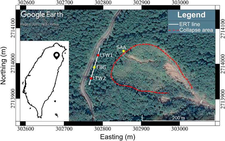
FIGURE 1. Location of the landslide potential area and layout of monitoring boreholes in the study area (modified from Google Earth). LTW1 is the location of an 84-m-deep borehole with ERT electrodes and LTW2 is the location of a 98-m-deep borehole with ERT electrodes and drilling core. SAA is the location of a borehole the shape acceleration array installed at the depths between 71.5 and 81.5 m; and FBG the borehole for the optical fiber Bragg grating pore pressure sensing array installed at the depths of 40, 50, and 60 m. A surface ERT line is also indicated by the white line joining through LTW1 and LTW2.

Geological Background

Taiwan formed approximately 5 million years ago in a still ongoing collision of tectonic plates (Suppe, 1981; Ho, 1986; Hall, 2002; Chiang et al., 2010) that lifts its young mountains and simultaneously generates innumerable earthquakes, is a densely populated island with 23 million inhabitants, and 70% of its area is mountainous. Its location in the tropical western Pacific Ocean means that typhoons frequently occur in summer, occasionally dropping meters of rain in just a few days. These characteristics of Taiwan make it one of the most landslide-prone countries in the world (Kornei, 2019). Landslides are complex geological phenomena with a high socio-economic impact in terms of loss of lives and damage and have indeed resulted in the loss of several lives and material belongings in Taiwan in recent years. Thus, landslide hazards require attention, including early warning systems and/or monitoring to aid in disaster preparation.

In the Lantai area, the terrain slope studied has an attitude of N29°E/30°E, and is located between the Chingshuihu Member and the Jentse Member of the Lushan formation (Figure 2). The geological profile is that the Jentse Member covers the Chingshuihu Member. According to field surveys and core drilling, there is a shear zone between the Jentse Member and the Chingshuihu Member. The lithology of the Lushan formation is composed of thick to massive slates with thin metamorphic sandstone or lenticular metamorphic sandstone, whereas the Chingshuihu Member contains thick black–gray shale with well-developed cleavages. Slates in the Chingshuihe Member is therefore easily eroded. Landslides thus often occur following heavy rainfalls or earthquakes in this steep terrain area (Lin M. L. et al., 2017). After completing the reinforcement works along the road in recent years, the ground deformation has slowed down. However, in the main collapse area (Figure 1), the GPS on the ground surface still continuously monitors the downward slope sliding situation. According to the monitoring data below 45 m, the accelerated displacements accompanied by heavy rainfalls or earthquakes had been frequently observed.

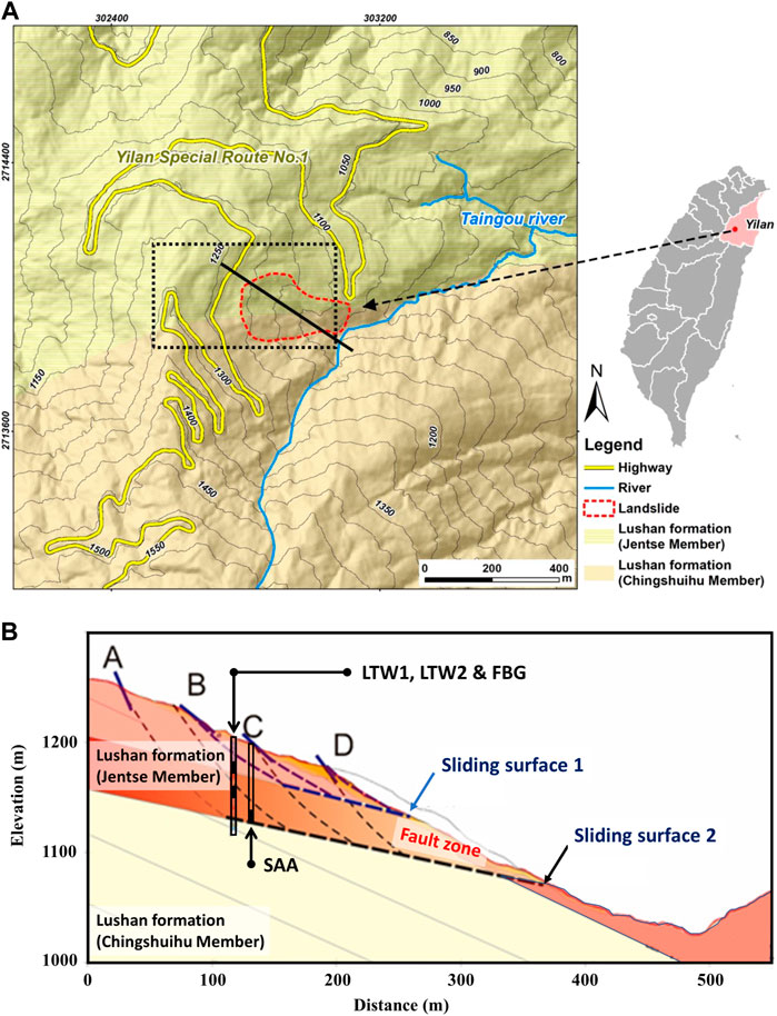
FIGURE 2. Geological map (A), together with a geological cross-section (B), in the Lantai area, Yilan Taiping Mountain, Northeast Taiwan. A-D was identified as four landslide scarps. The black line in the geological map denotes the location of the geological cross-section and the dotted rectangle shows the area in Figure 1.

Methodology and Data Processing

Electrical Resistivity Tomography Method

General ERT prospecting is widely applied to investigate electrical resistivity structures via the controlled injection of an electrical current into the subsurface and measurements of the potential difference between pairs of electrodes at the surface (AGI, 2009; Hsu et al., 2010; Chiang et al., 2012). The ERT method is based on Ohm’s law

using pairs of current electrodes to inject current (I) into the ground and potential electrodes to measure the potential difference (ΔV) between two arbitrary points within a specified distance (Figure 3).

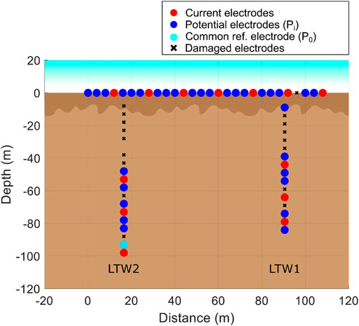
FIGURE 3. Schematics of the surface and borehole ERT electrodes used in this study. Some electrodes (in cross symbols) were damaged by the lightning strikes. For the details on the electrode array, please refer to The layout of the electrode and geotechnical monitoring arrays.

The electrical resistivity ρ is a measurement of the resistance R (=ΔV/I) through a cross-sectional area A with a wire of length l and can be formulated as

The apparent resistivity ρ_a in ERT can be derived from Eq. 3

where K is a geometric factor associated with the current and potential electrodes layouts. Recent developments in ERT instruments, including the R2MS used in this study, allow automatic switching measurements throughout different pairs of current and potential electrodes in a series of equally spaced distances laid out along surveying lines predefined (AGI, 2009; Hsu et al., 2010; Chang et al., 2012; Wang et al., 2015; Chang et al., 2018; Wang et al., 2020). Versatile instrumentation and electrode configurations enable effective 2D, 3D, and time-lapse ERT measurements. For a detailed description of the well-established ERT technique, we refer the readers to literature and many relevant references we cited.

The Layout of the Electrode and Geotechnical Monitoring Arrays

On the Lantai slope, several monitoring boreholes were drilled. They include the shape acceleration array (SAA), optical fiber Bragg grating (FBG) underground water pore pressure sensing array, two vertical linear arrays of electrodes in boreholes LTW1 and LTW2 (Figure 1). We will later describe the installation of the FBG pore pressure array in the following Hydrological water tank model for underground water

The SAA is a string of rigid segments separated by flexible joints. In each segment, it has a micro-electro-mechanical sensors system, which can measure the tilt angle relative to gravity’s direction and then convert the tilt angle into horizontal displacement by utilizing the triangular formula. We utilized the SAA to monitor the subsurface deformation by installing it into the borehole, labeled as SAA in Figure 1, at the depths from 71.5 to 81.5 m. The total length of SAA utilized is 10 m with the length of each segment is 0.5 m. The SAA installation depth normally depends on the borehole digging conditions and, in our case, was also judged from daily drilling log photos. The drilling jammed at the depths around 79 m and then showed intact rock after that. The drilling log photos furthermore illustrate fracture zones at the depths between 78 m and 80 m.

There are 16 and 18 electrodes installed in LTW1 and LTW2, respectively, whereas all electrodes are separated by 5 m. Additionally, on the joining line through LTW1 and LTW2, a linear array of 28 electrodes separated by 4 m has been installed on the surface (Figure 3). The total length of the surface ERT line was 108 m, and the depths of LTW1 and LTW2 were 84 and 98 m, respectively. The mixture electrode arrays were installed on the surface and in two boreholes to enhance the resolution of the electrical resistivity images in deep. According to field investigation and numerical simulation of slope stability, the studied slope could have different sliding surfaces distributed at various depths. Sliding surfaces below 45 m could exist as above mentioned in Geological background and deeper than 100 m not that active. Also considering the budget plan, this study therefore targets at the monitoring of physical properties of the slope body shallower than 100 m.

In those surface and borehole electrode arrays, the electrodes are arranged in an alternating way with part of the electrodes used for the electric current injections and the others for the electric potential measurements. When measuring electric potentials, one of the electrodes is selected as a common reference electric potential P₀ such that the electric potentials can be obtained as the potential differences between P₀ and other potential electrodes P_i (Figure 3). Consequently, the potential differences between every pair of potential electrodes can be estimated. With such electrode arrangement, named as the nontraditional hybrid array, conventional dipole-dipole, Wenner, Wenner-Schlumberger data, together with other four-pole data, can all be collected in a single measurement.

Data Acquisition and Processing

The electrical resistivity measurements were performed six times per day before July 2020. Then, for reducing the cost of lightning striking damage, the measurements were shrunk to two times per day, at 04:00 and 20:00, after July 2020. Figure 4 shows a chart of the electrical resistivity data process. The variations in the electrical resistivity data were strongly affected by rainfall; thus, for comparison in multiple ERT images, selecting a background period in the electrical resistivity data not affected by rainfall was necessary. We, therefore, select electrode pairs with high reproducibility as the stable background data. Eq. 4 was used to evaluate the quality (reproducibility) of the resistance data collected overall electrode pairs, where low $\stackrel{\rightharpoonup }{\text{Q}}$ values indicate high-quality data:

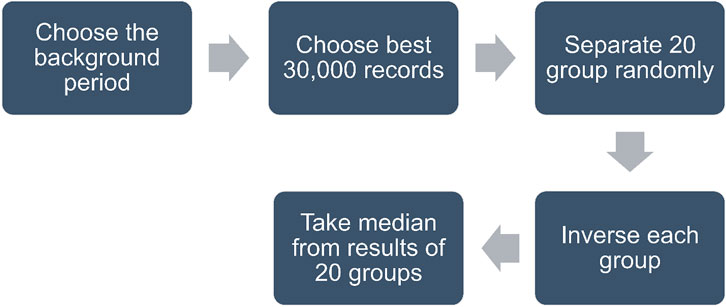
FIGURE 4. Flow chart of the processing procedure of our massive ERT data. For the details on ERT data processing, please refer to Data acquisition and processing.

N is the number of measurements selected in the background period; $\stackrel{\rightharpoonup }{{\text{Obs}}_{\text{i}}}$ denotes the measured resistances for every pair of current-potential electrodes, and median $\left(\stackrel{\rightharpoonup }{\text{Obs}}\right)$ indicates the median of the N measured resistivities.

After evaluating the data quality from July 7 to 12, 2020, we selected the best 30,000 data points among ∼180,000. We used the 2D inversion software EarthImager 2D developed by Advanced Geosciences Inc., United States (AGI, 2009). For dealing with the computing memory shortage, also benefiting from our extremely large amount of resistance data, we then randomly selected 20 subsets from the data population, each of which contains 6,000 data points. These 20 groups used the same parameters for the 2D inversions. The inversion procedure includes 1) fitness examination by using the root-mean-square (RMS) errors, 2) removals of the worst 5% resistance data with large RMS errors, and 3) repeated 2D inversion. The RMS error (AGI, 2009) is given by

and

Here, ${\text{ρ}}_{\text{i}}^{\text{means}}$ indicates the measured apparent resistivity, ${\text{ρ}}_{\text{i}}^{\text{pred}}$ indicates the inverted apparent resistivity, and N indicates the number of measurements. This procedure was repeated four times and could obtain a reasonable inverted image of the subsurface electrical structure for each subset. Having 20 inverted electrical images we took their median as the final ERT snapshot at each different time.

Relative Water Saturation Estimation

Archie’s (1942) law was applied to evaluate the water saturation:

where ρ is the resistivity of the rock, a is the tortuosity factor, Φ is the porosity of the rock, m is the cementation coefficient, S_w is the water saturation, n is the saturation exponent, and ρ_w is the water resistivity. The drilled core (Lin M. L. et al., 2017) revealed that most of the formations in the study area contain slate and that clay minerals can be ignored. Following Zhang et al. (2016), the relative water saturation (RWS) was defined as

where ${\text{S}}_{\text{w}}^{\text{k},\text{ t}1}$ is the degree of water saturation at the k-th mesh for time t1 and ${\text{S}}_{\text{w}}^{\text{k},\text{ t}2}$ for time t2, and ${\text{RWS}}^{\text{k},\text{ t}2,\text{t}1}$ indicates water saturation changes in percentage between the 2 days t1 and t2. Eq. 7 can be then substituted into Eq. 8 such that

where n is the saturation exponent and indicates the resistance ratio in porous water (Zhang et al., 2016). We had assumed that the tortuosity, cementation factors, rock porosity, and water resistivity do not change over short time scales in the order of tens of days and used n = 2.0 in this study to discuss the tendencies of the variations of RWS instead of its absolute values.

Rainfall Classifications Defined in This Study

Relations between the characteristics of rainfalls and the consequential landslides are often identified in landslide studies for early-warning thresholds. Most landslide studies have used precipitation magnitude and duration as parameters in the early warning system. Guzzetti et al. (2007) integrated from previous studies 25 parameters involving the duration and amount of rainfall events to define early warning signals for different rainfall scenarios. Segoni et al. (2018) suggested that landslide triggering factors could be statistically divided into three types: 1) rainfall intensity-duration curves (48.6%), 2) antecedent rainfall (26.8%), and 3) the accumulated rainfall and its duration (15.9%). Iverson (2000) simplified the Richards equation to evaluate the effect of rain infiltration on landslides at different time scales. However, relations between rainfall parameters and their warning levels are still controversial, and dividing rainfall events has remained an important scientific issue in the successful prediction of landslide occurrences.

This study is not aimed at the discussion of rainfall events and their classifications for the prediction of landslide occurrences. The rainfall classification here serves mainly as the baseline to calculate the variations in the time-lapse ERT images, to investigate the preferential areas to different extents for groundwater transport. We defined rainfall classifications using precipitation data from the Central Weather Bureau. The precipitation station was located approximately 400 m from the study area. Referring to Chen et al. (2005) and Melillo et al. (2015), the definitions are as follows: 1) a null rainfall is defined as 48 h of continuous rainfall of less than 4 mm, 2) a dry event is defined as over 72 h without precipitation, and 3) the starting and ending time of rainfall periods are determined according to the dry events. Figure 5 shows a schematic diagram of the rainfall classifications following these definitions, and Table 1 shows a schematic diagram of the rainfall classifications following these definitions, and Table 1 shows the rainfall classification durations in 2019. Rainfall events of less than and more than 10 days are referred to as short- and long-duration precipitation events, respectively. We have selected two exemplary cases from the rainfall classifications corresponding to one long-duration and one short-duration precipitation event to examine the variations in their electrical resistivity images with time and at different spatial scales.

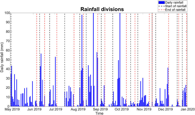
FIGURE 5. Rainfall classifications following the definitions described in Rainfall divisions defined in this study. All rainfall events are also listed in Table 1.

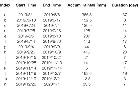
TABLE 1. Classifications of the rainfall events. The two events in red were selected for the case study.

Hydrological Water Tank Model for Underground Water

Installed alongside the ERT array, there is a linear array of the optical fiber Bragg grating (FBG) sensors for monitoring the underground pore water pressure. The design, instrumentation, and principles of the sensing technique are referred to by Huang et al. (2012). In the Lantai site, the array is installed in the FBG borehole shown in Figure 1. There are three serially connected working sensors at 40, 50, and 60 m, respectively, and their pressure sensing range is 400 kPa. The minimum gap distance was suggested to be longer than a couple of meters and 5 m was suggested in Huang, et al. (2012). For the FBG borehole, further drilling beyond 70 m became impossible because the drill head was frequently clamped by the surrounding hard fractured rocks. This condition may cause collapses of the borehole during sensor installation so that the drilling was halted. For the shallower installation, it may be above the underground water table and unsaturated so the reading of the sensor could be not trustable. Between the sensors, bentonite water sealing was realized to prevent direct water flows along the borehole and to ensure that the sensors correctly sense the pore water pressure at their depths in the aquifer. The raw data of the FBG sensing technique, after signal processing and digitalization of the FBG interrogators, are optical wavelengths, which are linearly proportional to the pore water pressure and the conversion factor is about 1 pm (wavelength) to 400 Pa, somewhat depending on the individual characteristics of the pressure sensor. The variation of the wavelength corresponds to the change of the spacing of the Bragg grating that is implemented in the optical fiber. The entire optical FBG system operates in the infrared wavelength range, about 1,450–1,600 nm. Inspecting the raw data of the three sensors, we found that the readings at 40 m had faster and occasionally daily responses, implying that this depth was probably about the underground water level and this confirms with the observation during the borehole drilling. On the other hand, the readings at 50 and 60 m are similar, indicating that they are likely in an aquifer with comparable material properties.

To compare the water content with the inverted electrical resistivity data, a semi-quantitative hydrological model is applied to map the FBG pore pressure data, taken at fixed positions, onto the effective underground water contents into a few representative layers. The main purpose of the hydrological model is to infer the water content in the layer above 40 m wherein it is usually not saturated and, to our knowledge, there is yet no long-term reliable technique available for direct measuring either the water content or pore water pressure.

The hydrological model used in this study is a simplified tank model. The model is used to simulate the rainfall-infiltration-runoff relations based on a series of hypothetically connected water tanks (Nash, 1957). There are many variants of the conceptual model, for example, a three serially connected tank model (Sugawara, 1961). The present tank model, on the other hand, is a simplified version with which contains two serially connected tanks (Lin S. E. et al., 2017; Kuo et al., 2021). In the model rainfall is the only input of water to the tanks. The water depth in the upper tank phenomenologically describes the water storage in the shallower layer of the unit landslide area and the lower tank is for the water storage in the deeper layer. The outflows of each tank are assumed linearly correlated with the depths of the water tanks. In total 12 parameters are to be determined in the model calibration process and the shuffled complex evolution scheme (SCE-UA, Duan et al., 1994) is applied for their calibration. In the process, the calibration target is to minimize the difference between the 60 m FBG pore pressure readings and the conceptual water depth of the second tank. This target function implies that the pressure measured at this depth is associated with the water storage in the deeper layer (the second tank). Without digressing into the calibration details, the explicit mathematical form of the target function, rainfall, and sensor data as well as the calibration results are relegated to the Supplementary Materials of the paper. From the former description on the pore pressure of the three depths, the referred deeper layer is likely to be below about 40 m. Nevertheless, because of the qualitative feature of the model, we cannot exactly specify the dividing depth between the deep and shallow layers but expect that it is in a vague range above 40 m. In Discussions, the depths of the individual tank, assumed in proportion to the water contents in the aquifer layers, are compared with the alternation of the electrical structures of the ERT images. For the full description and calibration results for the temporal period in the present paper, please refer to the Supplementary Materials.

Results

Electrical Resistivity Images and the Drill Core

Figure 6 shows the cross-section of an electrical resistivity image obtained on 21 Sept 2019, as an example, together with the drill core extracted from the borehole of LTW2. The top soil/colluvium layer can be seen between the surface and depths of 10 m and corresponds to the red-orange-yellow colors indicating high resistivity larger than 200 Ω-m. As suggested by the drill core, the depths of 10–30 and 60–100 m are fracture zones of slate formations and correspond to the blue-light blue colors indicating low resistivity less than 50 Ω-m. The depth of 30–60 m is likely associated with a compact slate formation and corresponds to the red-orange-yellow colors with, again, high resistivity larger than 200 Ω-m. The layered structure of the electrical resistivity image looks consistent with the drill core showing more details though. The ERT image was divided into six subzones (Figure 6) to discuss in the following sections the details of changes caused by rainfall events. The lowest resistivity appears in zone A, and the resistivity of zone B is similar to that of zone A at the same depths shallower than 30 m. Zones C and D have higher resistivity, which may be associated with those more intact slate formations implying that the hydraulic conductivity may be lower in the depths between 30 and 60 m. Zones E and F, with depths deeper than 60 m, have low resistivity features again. With the ERT images, we can focus on the spatiotemporal variations of the slate formation below the top soil/colluvium layer in the cross-section of the electrical resistivity image.

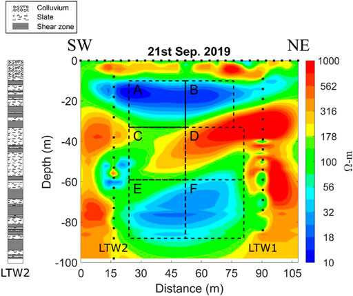
FIGURE 6. Cross-section of the electrical resistivity image and its subzones. The ERT image was divided into six subzones A-F, according to the depths and the resistivity values, for discussing in the text the details of the resistivity and RWS variations caused by rainfall events. For the depths, Zones A and B are shallower than 30 m; Zones C and D from 30 to 60 m; and Zones E and F deeper than 60 m. The lower resistivity values with several tens of ohm-meters appear in Zones A, B, E, and F while Zones C and D have the higher resistivity values with several hundreds of ohm-meters. The lithology column was also carefully registered from the drill core at the borehole of LTW2 (modified from Lin M. L. et al., 2017). Comparison with the lithology column of LTW2 suggests that the resistive Zones C and D may be associated with those more intact slate formations in the depths between 30 and 60 m.

Subzones of the Median Electrical Resistivity

Although the R2MS was several times struck by lightning during rainy days, the long-term variations in electrical resistivity have reliably shown smooth changes over time. Figure 7 presents the median electrical resistivity (MEER) of those subzones abovementioned, together with the daily rainfalls and the horizontal displacements measured by the SAA. We have taken the median value of electrical resistivities in model meshes within each subzone as the representative electrical resistivity to elucidate the temporal variations. Note that the MEER curves show slightly high roughness before July 2020, reflecting more frequent measurements taken in the early stage of this study. Overall, the MEER values show highly stable electrical resistivity measurements; it is also clear (Figure 7A) that, after July 2020, the MEER values decrease in zones A, B, and C, increase in zones D and E, and are steady in zone F. More detailed changes in electrical resistivity in terms of space will be discussed in Electrical resistivity changes due to the sliding event in summer 2020.

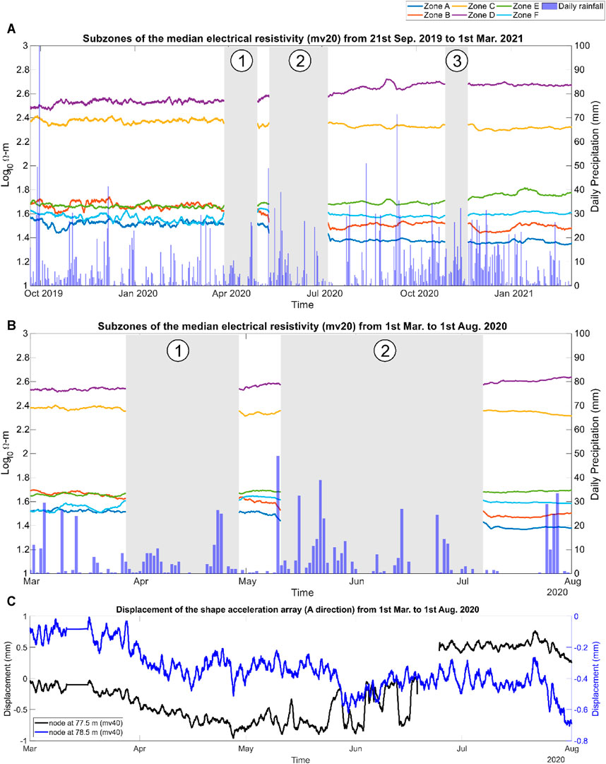
FIGURE 7. Time series of the median electrical resistivity (MEER) curves overlaid with the daily rainfall data. (A) Moving average of 20 measurements (mv20) of the MEER curves from 21 Sept 2019 to Mar 1, 2021. The dark blue line indicates Zone A, the orange line for Zone B, the yellow line Zone C, the purple line Zone D, the green line Zone E, and the light blue line for Zone F. Three gray zones labeled with Numbers 1-3 represent three periods when ERT measurements were interrupted due to the R2MS system damages caused by lightning strikes. (B) A zoom-in for the MEER curves from Mar 1 to Aug 1, 2020, to compare with the SAA data. (C) Horizontal displacement at the depths of 77.5 and 78.5 m is estimated from the SAA data.

Based on the fact that the MEER values in zones A and B exhibited extreme decreases and that of zone D increased after July 2020, and that those MEER changes look unrecoverable, we assume a small sliding event in summer 2020. Also, according to the SAA records at two different depths (Figure 7C), the displacement shows a gradually decreasing/creeping tendency from March through July at the depth of 78.5 m and a discontinuous decreasing trend starting from May following by an abrupt 1-mm jump close to the end of June at the depth of 77.5 m. The SAA data suggests that two different creeping units originally located at two depths of 77.5 and 78.5 m were likely tied together after that suspected event occurred at the end of June. Therefore, the SAA displacements show identical fluctuations at those two depths after June (Figure 7C).

In addition, the short-term MEER variations at different depths in Figure 7A are likely related to rain infiltration. This is discussed in more detail using RWS in Case study.

Case Study

In the following, we calculated the standard score, i.e., Z score, in statistics of the MEER values and the estimated RWS for two cases, one long-duration (Event l) and one short-duration (Event n) precipitation event in Table 1. The RWS calculations used reference ERT images from November 18 and December 25, 2019, for the long- and short-duration precipitation events, respectively.

Long-Duration Precipitation (Event l)

Figures 8A,B show similar MEER tendencies in zones A, B, and C for the long-duration precipitation (Event l in Table 1), where the MEER values increase with the precipitation and decrease with the end of the rainfall event. This feature indicates that the delayed electrical resistivity variations are likely related to the rainfall. The delayed time in zone C is the longest and is associated with the compact slate formation, as demonstrated by the drill core.

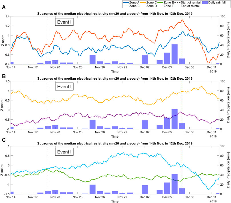
FIGURE 8. Standard score, i.e., Z-score, in statistics of the median electrical resistivity (MEER) time series for the long-duration precipitation event (Event l). Moving average for 20 measurements (mv20) of the MEER curves: (A) Zones A and B, (B) Zones C and D, and (C) Zones E and F.

Figure 9 shows the 5-days interval of the RWS values of the cross-sectional images and illustrates more detailed spatial structures of the electrical resistivity variations linked to water saturation for the long-duration precipitation Event l. RWS increases in the top soil/colluvium layer above zones A and B at the depth around 10 m and the near-surface RWS-increased zone is distributed over a horizontally wide spatial area (Figures 9A–D); then, RWS decreases with the end of the rainfall event and returns to its dry status (Figures 9E,F). The RWS distribution in the upper left corner of zone C at a depth of 30–50 m strikingly increases with the rainfall (Figures 9A–D). This was identified as a fracture zone according to the drill core, implying a superior channel for fluid. On the other hand, the RWS variations in zones D, E, and F show relatively slow increases after the rainfall (Figures 9E,F), implying that the formations wherein caused the precipitation infiltration to be delayed or that fluids in those zones were dominated by upstream groundwater.

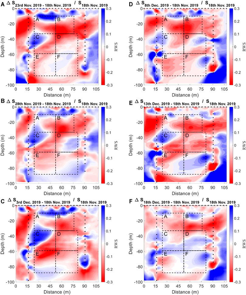
FIGURE 9. Cross-section of the relative water saturation (RWS) for the long-duration precipitation event based on the map for November 18, 2019, after (A) 5 days, (B) 10 days, (C) 15 days, (D) 20 days, (E) 25 days, and (F) 30 days. Blue shows increasing RWS estimated from the decreases in the electrical resistivities, whereas red shows decreasing RWS because of the resistivity increases.

Short-Duration Precipitation (Event n)

Figure 10 shows the standard scored MEER values for the short-duration precipitation event (Event n in Table 1). Zones A and C (Figures 10A,B) show similar MEER tendencies in three stages: a delayed decrease at the start of the rainfall event from Dec 26 to Dec 28, a first increase from Dec 28 to Dec 30, and then decrease from Dec 30 to Jan 1 during the rainfall event, and an increase after the end of the rainfall event from Jan 1 to Jan 8. The differences in the MEER variations between the long- and short-duration precipitation events might indicate the existence of different types of rainfall infiltration processes in this study area. However, the mechanism causing this difference is still uncertain and requires further exploration.

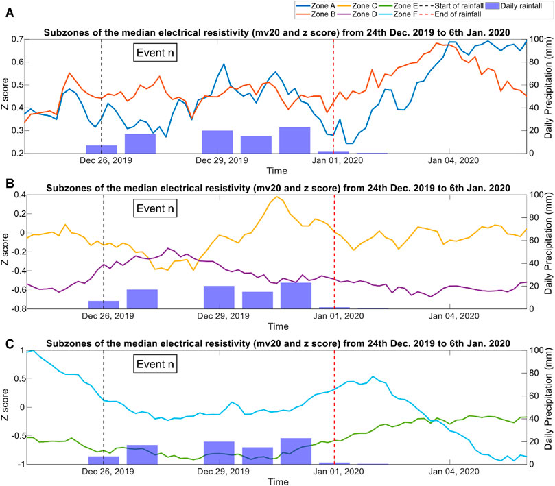
FIGURE 10. Z-score of the MEER time series for the short-duration precipitation event (Event n). Moving average for 20 measurements of the MEER curves: (A) Zones A and B, (B) Zones C and D, and (C) Zones E and F.

Figure 11 shows the 2-days interval of the RWS values of the cross-sectional images illustrating that the spatial electrical resistivity variations were linked to the water saturation for the short-duration precipitation Event n. RWS again increased in the top soil/colluvium layer above zones A and B and, compared with Event l, this near-surface RWS-increased zone was distributed over a relatively small spatial area (Figures 11A–D); RWS then slightly decreased with the end of the rainfall event (Figures 11E,F). The accumulated rainfall and daily rainfall in Event l were twice those in Event n. However, the RWS variations in zones D, E, and F were relatively larger in the short-duration event than in the long-duration event during the rainfall events and after the end of the rainfall periods, which is interesting. The deeper zones, D, E, and F, may not be able to significantly decrease their electrical resistivity with less rainfall, implying again that these deep, high RWS signals may have been affected by upstream groundwater brought in the early precipitation events.

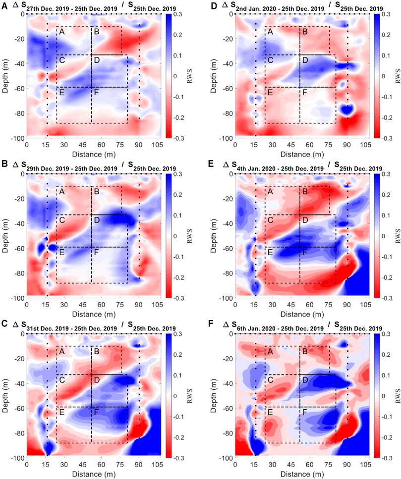
FIGURE 11. Cross-section of RWS for the short-duration precipitation event (Event n) based on the map for 04:00 on December 25, 2019, after (A) 2 days, (B) 4 days, (C) 6 days, (D) 8 days, (E) 10 days, and (F) 12 days. Blue shows increasing RWS, whereas red shows decreasing RWS.

Discussions

Electrical Resistivity Changes due to Water Storages

A water tank model is a simple half-quantitative hydraulic model (Sugawara, 1961) that divides geologic materials into multiple water tanks to model linear rainfall infiltration and runoff processes (Hydrological water tank model for underground water). Events l and n were set to have the same time windows to compare their electrical resistivity variations using a water tank model. Figure 12 shows the modeling results for two tanks with a side stream (Duan et al., 1994; Lin S. E. et al., 2017; Rustanto et al., 2017). The black and red lines show the water depths in the first and second tanks, respectively reflecting shallower and deeper water storage layers.

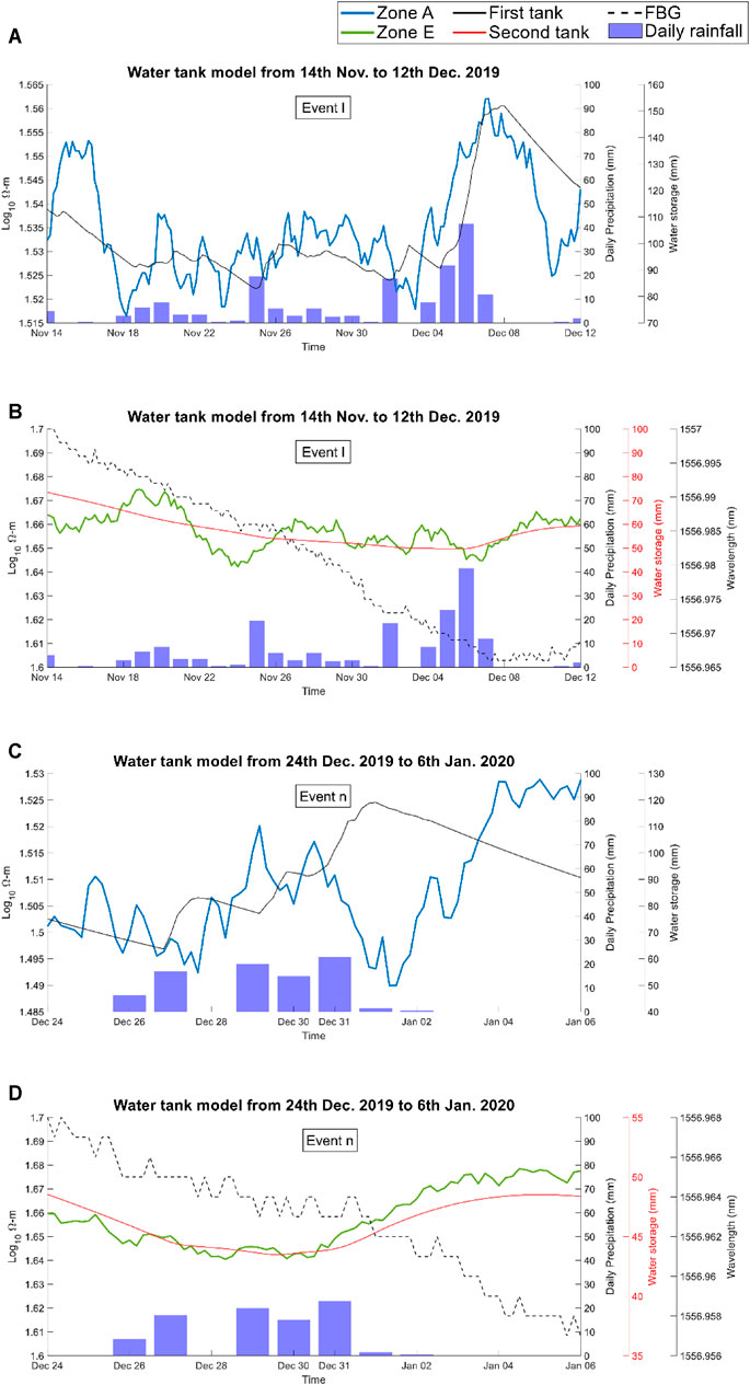
FIGURE 12. Comparison of the Z-score of the MEER time series, water tank model, and fiber Bragg grating sensor array (FBG) for the long-duration (Event l) and short-duration (Event n) precipitation events. The moving average for 20 measurements of the MEER curves. Event l: (A) Zone A and first tank model; (B) Zone E, second tank model, and the FBG. Event n: (C) Zone A and first tank; (D) Zone E, second tank model, and the FBG. Note that the shallower Zone A could be correlated with the shallower, first tank whereas the deeper Zone E with the deeper, second tank. The discrepancy between the MEER and the first curves in (c) for the short-duration Event n may imply the complexity of geological material in response to the magnitude of rainfall infiltration.

We found that the shallow tank can be mostly related to zone A whereas the deep tank to zone E. Echoing the existence of different types of rainfall infiltration processes in the study area, for the short-duration precipitation Event n, the trend between the MEER in zone E and the water storage in the deep tank remain good correlation while the relation between zone A and shallow tank became unclear after the end of rainfall (Figures 12C,D). The positive correlation between the MEER and the water storage, as shown in Figure 12, suggests water transport on the Lantai slope. As water flows deep outward from zone A or zone E, making the MEER values increasing, also increase the underlying water storages, calibrated by the FBG pore pressure data and estimated from the precipitation data. Note that the presence of less fluid makes it difficult to pass an electrical current through the geologic material. On the other hand, the tank model is a phenomenological hydrological model and the water depths in the tanks are thought to be qualitative indicators that do not represent the actual water depths in the aquifer layers. Nevertheless, this study provides strong evidence for the consistency among rainfall, pore pressure, and electrical resistivity data.

Electrical Resistivity Changes due to the Sliding Event in Summer 2020

A small sliding event is suspected to have occurred during the summer of 2020 according to the unrecoverable MEER changes and the SAA discontinuity as shown in Figure 7. Figure 13 shows the differences in the annual electrical resistivity variations between the periods before and after the suspected (if any) sliding event in December, January, and February. The electrical resistivities appear to mostly show decreases (Figures 13A–C) in these 3 months, except at a depth of around 60 m in zones C and D. An electrical-resistivity-increased layer appears around 60 m that indicates the geologic property has been likely changed due to the sliding event. Since the SAA data suggests that the sliding surface could be located at ∼78 m, the geological material above seems less porous after the shearing process of the sliding event. On the other hand, an electrical-resistivity-decreased zone appears to lay above at around 40 m deep, suggesting the material has possibly become more fractured. Noted that both the electrical-resistivity-decreased and increased zones abovementioned are corresponding to the original high resistivity structure located at zones C and D (Figure 6), implying that a new sliding surface may be growing in the area of the depths between 40 and 60 m. Observing the differences in precipitation for these 3 months, indeed, rainfall infiltration has some minor effects on zones A, B, E, and F, slightly lowering electrical resistivities. It is also important to exam the resolution to the summer 2020 event under the ERT array we used in the field. We, therefore, did the ERT forward and inversion calculations with two synthetic models before and after the sliding event (Figures 14A,B), wherein the shallower part of the mid-high-resistivity layer in the depths between 30 and 60 m became more conductive after the event and the deeper part more resistive. With resistance data synthesized by the same electrode array as we used in the field, the numerical experiment of time-lapse ERT can recover the changes in electrical resistivities due to the hypothetical sliding event (Figure 14C).

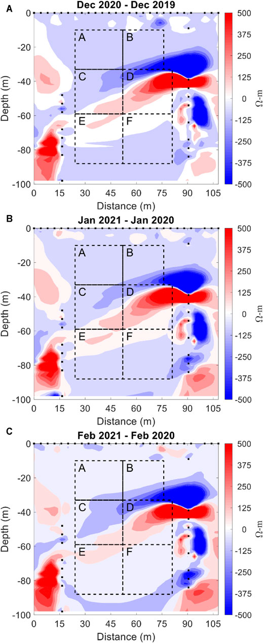
FIGURE 13. Comparison of the electrical resistivity images for the months before and after a suspected creeping event. Differences in the electrical resistivity (A) between December 2019 and 2020, (B) between January 2020 and 2021, and (C) between February 2020 and 2021. For details please refer to the explanation in Electrical resistivity changes due to the sliding event in summer 2020.

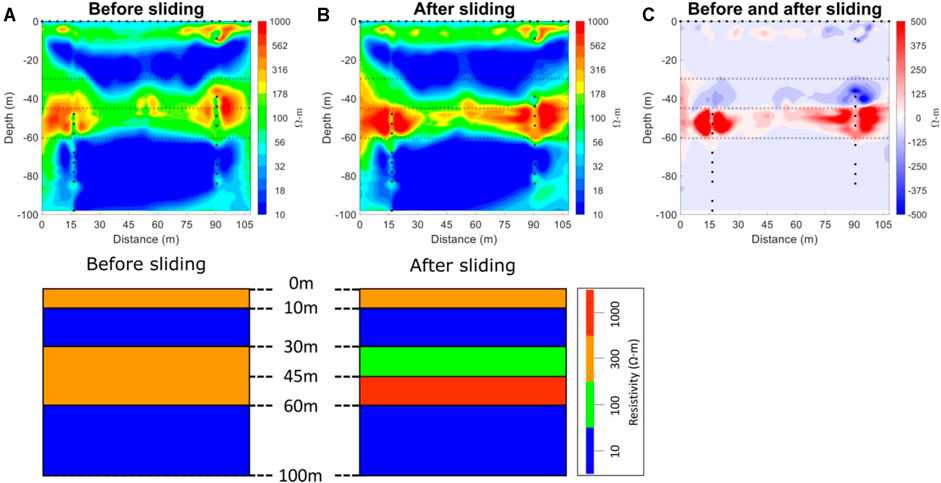
FIGURE 14. Numerical modeling to test the resolving capability of the ERT electrode array used in the field. We assume that, due to a hypothetical sliding event, the shallower part of the mid-high-resistivity layer in the depths between 30 and 60 m became more conductive and the deeper part more resistive. Shown in (A) and (B) are the synthetic resistivity (lower panels) and their inverted (upper panels) models before and after, respectively, the sliding event. (C) Differences in time-lapse ERT images can recover the underground changes, caused by that hypothetical event, in electrical resistivities as we observed in the field experiments.

Conclusion

We presented in this study the results of time-lapse ERT measurements in the Lantai slope, Yilan Taiping Mountain, Northeast Taiwan. The boundaries of the cross-sectional electrical resistivity images are mostly consistent with the drill core, suggesting that the ERT can image in a relatively macroscopic viewpoint geologic structures in potential landslide areas. The electrical resistivity profile in the study area shows a layered structure consisting of a resistive top soil/colluvium layer between the surface and 10 m depth, a conductive and fractured layer at 10–30 m depth, a resistive and compact slate formation from 30 to 60 m depth and, again, a conductive and fractured layer down to the depth of 100 m.

We also demonstrated that the spatiotemporal responses of the slope underground during rainfall events could be investigated by means of the time-lapse ERT monitoring technique. Integrating data from the ERT, the shape acceleration array, and the underground water pore pressure sensing array, we have shown different rainfall infiltration processes in the studied slope and possibly detected a small sliding/deformation event in summer 2020. The rainfall infiltration processes could be complicated in response to the duration and magnitude of precipitation. During the observation period, we have not observed a substantial landslide that could be sensed in the ground, but the suspected small slide/deformation might have caused detectable changes in the electrical resistivity data and the borehole SAA data as well. Before registering valuable multi-physical data of a notable landslide event and understanding the hydro-mechanical conditions of landslides, we believe that inspection of integrated data as shown in this study may be also helpful to improve quantitative analyses for the physical mechanism of landslide, thus to contribute the building blocks of landslide alert systems.

Data Availability Statement

The original contributions presented in the study are included in the article/Supplementary Material, further inquiries can be directed to the corresponding author.

Author Contributions

W-NT: Conceptualization, Writing-Original Draft, Validation, Investigation, Data Curation, Visualization; C-CC: Conceptualization, Methodology, Investigation, Data Curation, Supervision, Funding acquisition; C-WC: Writing-Original Draft, Investigation, Editing, Supervision; P-YC: Methodology, Resources; C-YK: Methodology, Resources; K-LW: Resources; M-LL: Resources; R-FC: Resources.

Funding

This study was supported by the Ministry of Science and Technology, R.O.C., and the Soil and Water Conservation Bureau Council of Agriculture, Executive Yuan, R.O.C., under grant nos. 104-2119-M-006-008, 105-2119-M-006-010, and 106-2119-M-006-009.

Conflict of Interest

The authors declare that the research was conducted in the absence of any commercial or financial relationships that could be construed as a potential conflict of interest.

Publisher’s Note

All claims expressed in this article are solely those of the authors and do not necessarily represent those of their affiliated organizations, or those of the publisher, the editors and the reviewers. Any product that may be evaluated in this article, or claim that may be made by its manufacturer, is not guaranteed or endorsed by the publisher.

Acknowledgments

We greatly thank the permission of the Taipingshan National Forest Recreation under the jurisdiction of the Luodong Forest District Office for the study.

Supplementary Material

The Supplementary Material for this article can be found online at: https://www.frontiersin.org/articles/10.3389/feart.2021.737271/full#supplementary-material

References

AGI (2009). Instruction manual for EarthImager 2D. Austin, Texas, USA: Advanced Geosciences, Inc. Version 2.4. 0.
Archie, G. E. (1942). The electrical resistivity log as an aid in determining some reservoir characteristics. Trans. AIME 146, 54–62. doi:10.2118/942054-G
Bishop, A. W. (1960). The principle of effective stress. Norw. Geotech. Inst. Publ. 32, 1–5. doi:10.1021/ac60166a763
Cassiani, G., Boaga, J., Vanella, D., Perri, M. T., and Consoli, S. (2015). Monitoring and modelling of soil-plant interactions: the joint use of ERT, sap flow and eddy covariance data to characterize the volume of an orange tree root zone. Hydrol. Earth Syst. Sci. 19 (5), 2213–2225. doi:10.5194/hess-19-2213-2015
Chambers, J. E., Wilkinson, P. B., Weller, A. L., Meldrum, P. I., Ogilvy, R. D., and Caunt, S. (2007). Mineshaft imaging using surface and crosshole 3D electrical resistivity tomography: A case history from the East Pennine Coalfield, UK. J. Appl. Geophys. 62, 324–337. doi:10.1016/j.jappgeo.2007.03.004
Chang, P.-Y., Chen, C.-c., Chang, S.-K., Wang, T.-B., Wang, C.-Y., and Hsu, S.-K. (2012). An investigation into the debris flow induced by Typhoon Morakot in the Siaolin area, southern Taiwan, using the electrical resistivity imaging method. Geophys. J. Int. 188, 1012–1024. doi:10.1111/j.1365-246X.2011.05310.x
Chang, P.-Y., Huang, W.-J., Chen, C.-C., Hsu, H.-l., Yen, I.-C., Ho, G.-R., et al. (2018). Probing the frontal deformation zone of the Chihshang Fault with boreholes and high-resolution electrical resistivity imaging methods: A case study at the Dapo site in eastern Taiwan. J. Appl. Geophys. 153, 127–135. doi:10.1016/j.jappgeo.2018.04.006
Chen, W., Li, Y., and Wu, H. (2005). Study of judging debris flow occurrence by combing the physiographical factors and rainfall condition-Chen-Yu-Lan stream watershed as an example. J. Taiwan Geogr. Info. Sci. 2, 27–44. (in Chinese). doi:10.29790/JTGIS.200504.0003
Chiang, C.-W., Chen, C.-C., Unsworth, M., Bertrand, E., Chen, C.-S., Kieu, T. D., et al. (2010). The deep electrical structure of southern Taiwan and its tectonic implications. Terr. Atmos. Ocean. Sci. 21 (6), 879–895. doi:10.3319/tao.2010.02.25.01(t)
Chiang, C.-W., Goto, T.-n., Mikada, H., Chen, C.-C., and Hsu, S.-K. (2012). Sensitivity of Deep-Towed Marine Electrical Resistivity Imaging Using Two-Dimensional Inversion: A Case Study on Methane Hydrate. Terr. Atmos. Ocean. Sci. 23 (6), 725–732. doi:10.3319/tao.2012.06.19.01(t)
Chiang, C.-W., Hsu, H.-L., and Chen, C.-C. (2015). An Investigation of the 3D Electrical Resistivity Structure in the Chingshui Geothermal Area, NE Taiwan. Terr. Atmos. Ocean. Sci. 26 (3), 269–281. doi:10.3319/tao.2014.12.09.01(t)
Crosta, G. (1998). Regionalization of rainfall thresholds: an aid to landslide hazard evaluation. Environ. Geology. 35 (2-3), 131–145. doi:10.1007/s002540050300
Dai, F. C., and Lee, C. F. (2002). Landslide characteristics and, slope instability modeling using GIS, Lantau Island, Hong Kong. Geomorphology 42 (3-4), 213–228. doi:10.1016/s0169-555x(01)00087-3
Daily, W., Ramirez, A., Labrecque, D., and Nitao, J. (1992). Electrical resistivity tomography of vadose water movement. Water Resour. Res. 28, 1429–1442. doi:10.1029/91wr03087
Descloitres, M., Ruiz, L., Sekhar, M., Legchenko, A., Braun, J.-J., Mohan Kumar, M. S., et al. (2008). Characterization of seasonal local recharge using electrical resistivity tomography and magnetic resonance sounding. Hydrol. Process. 22, 384–394. doi:10.1002/hyp.6608
Duan, Q. Y., Sorooshian, S., and Gupta, V. K. (1994). Optimal use of the sce-ua global optimization method for calibrating watershed models. J. Hydrol. 158 (3-4), 265–284. doi:10.1016/0022-1694(94)90057-4
Guzzetti, F., Peruccacci, S., Rossi, M., and Stark, C. P. (2007). Rainfall thresholds for the initiation of landslides in central and southern Europe. Meteorol. Atmos. Phys. 98, 239–267. doi:10.1007/s00703-007-0262-7
Hall, R. (2002). Cenozoic geological and plate tectonic evolution of SE Asia and the SW Pacific: computer-based reconstructions, model and animations. J. Asian Earth Sci. 20 (4), 353–431. doi:10.1016/s1367-9120(01)00069-4
Ho, C. S. (1986). A synthesis of the geologic evolution of Taiwan. Tectonophysics 125, 1–16. doi:10.1016/0040-1951(86)90004-1
Hsu, H.-L., Yanites, B. J., Chen, C.-c., and Chen, Y.-G. (2010). Bedrock detection using 2D electrical resistivity imaging along the Peikang River, central Taiwan. Geomorphology 114, 406–414. doi:10.1016/j.geomorph.2009.08.004
Huang, A.-B., Lee, J.-T., Ho, Y.-T., Chiu, Y.-F., and Cheng, S.-Y. (2012). Stability monitoring of rainfall-induced deep landslides through pore pressure profile measurements. Soils and Foundations 52 (4), 737–747. doi:10.1016/j.sandf.2012.07.013
Iverson, R. M. (2000). Landslide triggering by rain infiltration. Water Resour. Res. 36, 1897–1910. doi:10.1029/2000WR900090
Jongmans, D., and Garambois, S. (2007). Geophysical investigation of landslides : a review. Bull. Soc. Géol. Fr. 178 (2), 101–112. doi:10.2113/gssgfbull.178.2.101
Kornei, K. (2019). A massive experiment in Taiwan aims to reveal landslides' surprising effect on the climate. Science 366, 938–940. doi:10.1126/science.aba2653
Kuo, C. Y., Lin, S. E., Chen, R. F., Hsu, Y. J., Chang, K. J., Lee, S. P., et al. (2021). Occurences of deep-seated creeping landslides in accordance with hydrological water storages in catchments. Front. Earth Sci. submitted.
Kuras, O., Pritchard, J. D., Meldrum, P. I., Chambers, J. E., Wilkinson, P. B., Ogilvy, R. D., et al. (2009). Monitoring hydraulic processes with automated time-lapse electrical resistivity tomography (ALERT). Comptes Rendus Geosci. 341 (10-11), 868–885. doi:10.1016/j.crte.2009.07.010
Lin, M. L., Chena, T. W., and Hsia, K. C. (2017a). Evolution and stability analysis of a deep-seated landslide in Lantai area, Taiwan. Geotechnical Hazard. Mitigations: Experiment, Theor. Practice-Proceedings 5th Int. Conf. Geotechnical Eng. Disaster Mitigation Rehabil., 391–402. doi:10.6140/9789864371419.201710.0034
Lin, S. E., Chan, Y. H., Kuo, C. Y., Chen, R. F., Hsu, Y. J., Chang, K. J., et al. (2017b). The use of a hydrological catchment model to determine the occurrence of temporal creeping in deep-seated landslides. J. Chin. Soil Water Conserv. 48 (4), 153–162. doi:10.29417/JCSWC.201712_48(4).0001
Maillol, J. M., Seguin, M.-K., Gupta, O. P., Akhauri, H. M., and Sen, N. (1999). Electrical resistivity tomography survey for delineating uncharted mine galleries in West Bengal, India*. Geophys. Prospecting 47, 103–116. doi:10.1046/j.1365-2478.1999.00126.x
Melillo, M., Brunetti, M. T., Peruccacci, S., Gariano, S. L., and Guzzetti, F. (2015). An algorithm for the objective reconstruction of rainfall events responsible for landslides. Landslides 12, 311–320. doi:10.1007/s10346-014-0471-3
Morgenstern, N. R., and Price, V. E. (1965). The analysis of the stability of general slip surfaces. Géotechnique 15 (1), 79–93. doi:10.1680/geot.1965.15.1.79
Müller, K., Vanderborght, J., Englert, A., Kemna, A., Huisman, J. A., Rings, J., et al. (2010). Imaging and characterization of solute transport during two tracer tests in a shallow aquifer using electrical resistivity tomography and multilevel groundwater samplers. Water Resour. Res. 46, 23. doi:10.1029/2008wr007595
Nash, J. E. (1957). The form of the instantaneous unit hydrograph. Int. Ass. Sci. Hydrol. 3, 114–121.
Oldenborger, G. A., Knoll, M. D., Routh, P. S., and LaBrecque, D. J. (2007). Time-lapse ERT monitoring of an injection/withdrawal experiment in a shallow unconfined aquifer. Geophysics 72 (4), F177–F187. doi:10.1190/1.2734365
Palis, E., Lebourg, T., Vidal, M., Levy, C., Tric, E., and Hernandez, M. (2017). Multiyear time-lapse ERT to study short- and long-term landslide hydrological dynamics. Landslides 14, 1333–1343. doi:10.1007/s10346-016-0791-6
Perrone, A., Lapenna, V., and Piscitelli, S. (2014). Electrical resistivity tomography technique for landslide investigation: A review. Earth-Science Rev. 135, 65–82. doi:10.1016/j.earscirev.2014.04.002
Petley, D. N., Mantovani, F., Bulmer, M. H., and Zannoni, A. (2005). The use of surface monitoring data for the interpretation of landslide movement patterns. Geomorphology 66, 133–147. doi:10.1016/j.geomorph.2004.09.011
Rustanto, A., Booij, M. J., Wösten, H., and Hoekstra, A. Y. (2017). Application and recalibration of soil water retention pedotransfer functions in a tropical upstream catchment: case study in Bengawan Solo, Indonesia. J. Hydrol. Hydromech. 65 (3), 307–320. doi:10.1515/johh-2017-0020
Segoni, S., Piciullo, L., and Gariano, S. L. (2018). A review of the recent literature on rainfall thresholds for landslide occurrence. Landslides 15, 1483–1501. doi:10.1007/s10346-018-0966-4
Sugawara, M. (1961). On the analysis of runoff structure about several Japanese rivers, Japanese. J. Geophys. 2, 210–216.
Suppe, J. (1981). Mechanics of mountain-building and metamorphism in Taiwan. Mem. Geol. Soc. China 4, 67–89.
Tang, J.-T., Zhang, J.-F., Feng, B., Lin, J.-Y., and Liu, C.-S. (2007). Determination of borders for resistive oil and gas reservoirs by deviation rate using the hole-to-surface resistivity method. Chin. J. Geophys. 50, 790–795. doi:10.1002/cjg2.1094
Wang, T.-P., Chen, C.-C., Tong, L.-T., Chang, P.-Y., Chen, Y.-C., Dong, T.-H., et al. (2015). Applying FDEM, ERT and GPR at a site with soil contamination: A case study. J. Appl. Geophys. 121, 21–30. doi:10.1016/j.jappgeo.2015.07.005
Wang, T.-P., Chen, Y.-T., Chen, C.-C., Tung, T.-H., Cheng, S.-N., and Yu, C.-Y. (2020). Application of cross-hole electrical resistivity tomography to groundwater contaminated remediation site. Terr. Atmos. Ocean. Sci. 31, 507–521. doi:10.3319/TAO.2019.06.17.01
Yeh, H.-F., Lin, H.-I., Wu, C.-S., Hsu, K.-C., Lee, J.-W., and Lee, C.-H. (2015). Electrical resistivity tomography applied to groundwater aquifer at downstream of Chih-Ben Creek basin, Taiwan. Environ. Earth Sci. 73, 4681–4687. doi:10.1007/s12665-014-3752-1
Zhang, G., Lü, Q.-T., Zhang, G.-B., Lin, P.-R., Jia, Z.-Y., and Suo, K. (2018). Joint Interpretation of Geological, Magnetic, AMT, and ERT Data for Mineral Exploration in the Northeast of Inner Mongolia, China. Pure Appl. Geophys. 175, 989–1002. doi:10.1007/s00024-017-1733-5
Keywords: time-lapse electrical resistivity tomography, rainfall infiltration, water saturation, landslide, hazard mitigation
Citation: Tsai W-N, Chen C-C, Chiang C-W, Chen P-Y, Kuo C-Y, Wang K-L, Lin M-L and Chen R-F (2021) Electrical Resistivity Tomography (ERT) Monitoring for Landslides: Case Study in the Lantai Area, Yilan Taiping Mountain, Northeast Taiwan. Front. Earth Sci. 9:737271. doi: 10.3389/feart.2021.737271
Received: 06 July 2021; Accepted: 23 September 2021;
Published: 08 October 2021.
Edited by:
Chong Xu, Ministry of Emergency Management, ChinaReviewed by:
Changdong Li, China University of Geosciences Wuhan, ChinaJoern Lauterjung, German Research Centre for Geosciences, Germany
Copyright © 2021 Tsai, Chen, Chiang, Chen, Kuo, Wang, Lin and Chen. This is an open-access article distributed under the terms of the Creative Commons Attribution License (CC BY). The use, distribution or reproduction in other forums is permitted, provided the original author(s) and the copyright owner(s) are credited and that the original publication in this journal is cited, in accordance with accepted academic practice. No use, distribution or reproduction is permitted which does not comply with these terms.
*Correspondence: Chih-Wen Chiang, zjiang@ntou.edu.tw