Cellular Self-Structuring and Turbulent Behaviors in Atmospheric Laminar Channels

Introduction

In order to better introduce and contextualize this manuscript, our past works on the subject must be first detailed and the theoretical and practical results obtained must be explained. In the first of these works, a multifractal approach of the turbulent atmosphere is generally considered, whereby implementing this theoretical framework through non-differentiable functions in the form of scale relativity theory, the fractal minimal vortex of an instance of turbulent flow is obtained (Roşu et al., 2020). This leads to equations that describe the minimal vortex itself, and the velocity fields that compose it. Once this theoretical framework has been established, certain relations are exploited in order to calculate turbulent diffusion using lidar data, and the resulting profiles are found to be in agreement with other associated published works (Roșu et al., 2020). In the second paper, the connection between atmospheric multifractal theory and lidar data is further explored by improving a turbulence cascade evolution model so that each vortex presents an increasing Hausdorff dimension (Roșu et al., 2021a). In the third paper, the improved model is found to be resulting from a gauge produced by scaling theories, which implies that it is part of a large class of possible models – most notably, however, the model is coupled to a Galerkin decomposition of the Navier-Stokes equations which produces a logistic map-type evolution equation of velocity modes (Roșu et al., 2021b). Then, this coupling makes it possible to identify quasi-laminar or fully laminar regions in atmospheric profiles, leading to “laminar channel” structures that show either ascending or descending behavior (Roșu et al., 2021b). Finally, developments were also made towards reducing the number of initial parameters that the improved turbulence cascade evolution model requires (Roșu et al., 2021b). In the current work, the particularities of these laminar channels, and laminarity in general in the context of multifractality, self-structuring of atmospheric entities and the implications of self-structuring shall be the focus of our analysis.

The Motion Operator as the Scale Covariant Derivative

Since the atmosphere both structurally and functionally can be assimilated to a multifractal object, its dynamics are characterized in the frame of scale relativity theory through the scale covariance derivative (Roșu et al., 2020; Roșu et al., 2021a; Roșu et al., 2021b):

where:

and:

-$\mathit{F}$ is a fractal/multifractal function

-$x^r$ is the fractal spatial coordinate

-$t$ is the time, non-fractal, playing also the role of an affine parameter of the trajectories

-$dt$ is the scale resolution

-$f\left(\alpha \right)$ defines the singularity spectrum of order $\alpha$, where $\alpha$ is the singularity index which is a functional of the fractal dimension $D_F$ in the form $\alpha \left(D_F\right)$

-${\widehat{V}}^r$ is the complex velocity

-$V_D^r$ is the differentiable velocity independent on $dt$

-$V_F^r$ is the non-differentiable velocity dependent on $dt$

-$D^{rp}$ is a constant tensor corresponding to the differentiable-non-differentiable transition

-${\lambda }_{-}^r{\lambda }_{-}^p$ respectively ${\lambda }_{+}^r{\lambda }_{+}^p$ are constant vectors corresponding to the backward, respectively forward differentiable-non-differentiable processes

In the case of atmosphere dynamics through stochastic fractalization/multifractalization (for example, Markov-type stochastic processes, non-Markov stochastic processes, etc.) we may distinguish the following patterns:

1) patterns which include atmospheric processes through homogenous behaviors characterized by a single fractal dimension, that possess the same scaling properties in any time interval (monofractal) (Jackson, 1989; Cristescu, 2008);

2) patterns which include atmospheric processes through non-homogenous behaviors characterized simultaneously by multiple fractal dimensions (multifractal). Thus, the spectrum $f\left(\alpha \right)$ can permit the identification of a universality pattern in the domain of atmosphere dynamics, even when these patterns appear different (Jackson, 1989; Cristescu, 2008).

Then, instead of “working” with a single variable described by a strict, non-differentiable function, it is possible to “operate” only with approximations of this mathematical function, obtained by averaging them on different scale resolutions. As a consequence, any variable purposed to describe atmospheric processes will still perform as the limit of a family of mathematical functions, this being non-differentiable for null scale resolutions and differentiable otherwise (Nottale, 2011; Merches and Agop, 2015; Agop and Paun, 2017). There are many ways to define the fractal dimension: Kolmogorov, Hausdorff-Besikovitch, etc. definitions, but once one chosen to employ it in the atmosphere dynamics, it should be constant and arbitrary for the entirety of our analysis (Mandelbrot, 1982; Jackson, 1989; Cristescu, 2008).

Conservation Laws of the Multifractal Flows

Now, considering the scale covariance principle and using the operator in Eq. 1 applied to the complex velocities from Eq. 2, without any constraints, the multifractal conservation law of the specific momentum can be written in the form:

where ${\partial }_{\mathbf{t}}{\widehat{\mathit{V}}}^{\mathit{i}}$ represents local multifractal acceleration, ${\widehat{\mathit{V}}}^r{\partial }_r{\widehat{V}}^i$ represents multifractal convection and $D^{rp}{\partial }_r{\partial }_p{\widehat{V}}^i$ multifractal dissipation (Roșu et al., 2020; Roșu et al., 2021a; Roșu et al., 2021b). Thus, in every point of the given motion trajectory multifractal inertia, multifractal convection and multifractal dissipation are balanced. In these conditions, separating the atmospheric dynamics on scale resolutions both at differentiable and non-differentiable scale resolutions, Eq. 3 can be dissociated in two equations:

which reflects the fact that the motions of the atmospheric entities involve interdependent complex mechanisms, both at differential and non-differential scale resolutions.

Since, usually, multifractalization proves to be reducible to stochasticity, next we will consider the case of multifractalization by Markov-type stochastic processes, which imply the following conditions:

where $\lambda \left(\mu \right)$ are specific coefficients associated to the multifractal to non-multifractal transitions and ${\delta }^{ir}$ is Kronecker’s pseudo-tensor.

In conditions expressed by Eq. 6, Eq. 3 becomes:

in which case the separation of the atmospheric dynamics on scale resolutions implies the functionality of the following differential equations for the velocity fields:

For laminar movements of atmospheric entities, the complex velocity fields given by Eq. 2a become:

with $\text{Ψ}$ the states function. If $\text{Ψ}$ has the form:

where $\sqrt{\rho }$ is the amplitude and $s$ the phase, the complex velocity field transforms into:

It is also possible to see from the previous equations that $\sqrt{\mathbf{\rho }}$ is in fact the state density of ${\widehat{V}}^i$. The previous equation leads to the determination of real velocity fields:

By Eqs 13–15, Eq. 8 implies the multifractal hydrodynamic equations:

where with $Q$ is denoted the specific multifractal potential:

The Eq. 16 is the multifractal conservation law of the specific momentum, while Eq. 17 is the multifractal conservation law of the states density. The potential $\mathbf{Q}$ expressed by Eq. 18 requires the multifractal specific force:

which quantifies the multifractality degrees of the motion trajectories of the atmospheric particles.

Coherences in Stationary Atmospheric Dynamics Through a “Hidden” Symmetry

The existence of this force will be considered as the “trigger” of the atmospheric processes that lead to turbulence. If the specific multifractal potential is constant, or if in the one-dimensional case the following condition is satisfied:

where $\epsilon$ is a multifractal integration constant. Then, according to a special operational procedure, a multifractal hidden symmetry of $SL(2,R)$ multifractal type becomes functional. Indeed, let us rewrite the general solution of Eq. 20 as:

where $h$ is a complex amplitude, $\overline{h}$ is its complex conjugate, $\Phi$ is a specific phase and $x$ the spatial coordinate. Then, $h$ and $\Phi$ brand each entity of the atmosphere which has as a general characteristic Eq. 20, and thus the same $k$.

The quantities $h$, $\overline{h}$ and $\Phi$ give initial conditions which are not the same for every atmospheric entity; more precisely, these various entities find themselves in different states. The following problem is highlighted – is it possible to emit “a priori” a connection between $h$, $\overline{h}$ and $e^{i\left(kx+\Phi \right)}$ belonging to different atmospheric entities? The fact that Eq. 22 is a solution of Eq. 20 allows an affirmative answer to this question. Indeed, Eq. 22 possesses a “hidden” symmetry expressed through the homographic group: a ratio $\sigma \left(x\right)$ of two solutions of Eq. 20 is a solution of Schwartz’s equation:

where:

and $\left\{\sigma , x\right\}$ is the Schwartzian of the function $\sigma$ in relation to $x$ (Mihaileanu, 1972; Agop and Mazilu, 2011). Equation 23 is invariant to the homographic transformation of $\sigma \left(x\right)$: any such function is in itself a solution of Eq. 23. Since homography characterizes line projectivity, it is then possible to affirm that the ratio of two solutions of Eq. 20 is a projective parameter for the totality of atmospheric entities sharing the same $k$. A useful projective parameter can be constructed, which is in biunivocal correspondence with any atmospheric entity.

First, let us observe a “universal” projective parameter – the ratio of the fundamental solutions of Eq. 20 gives:

Every homographic function of this type will be a projective parameter. Among others, the function:

has the advantage to be specific to every atmospheric entity. This is not all; let another function:

which is specific to a different atmospheric entity. The fact that Eq. 26 and Eq. 27 are solutions of Eq. 23 shows that between them there is the homographic relation:

which implies the transformations group:

Equation 29 can be assimilated to a group of synchronisms between the diverse entities of the atmosphere, a process which includes synchronization between the amplitudes and phases of the atmospheric entities.

The structure of this group is typical of $SL\left(2R\right)$, i.e.:

where $B^1$, $B^2$ and $B^3$ are the infinitesimal generators of the groups:

This group admits the absolute invariant differentials:

and the 2-form (the metric):

In real terms:

and for:

the connection with Poincaré representation of the Lobachevsky plane can be obtained. Indeed, the metric is a three-dimensional Lorentz structure:

This metric reduces to that of Poincaré in case where ${\text{Ω}}^1\equiv 0$ which defines the variable $\theta$ as the “angle of parallelism” of the hyperbolic planes (the connections) (Agop and Mazilu, 2011). In fact, recalling that:

represents the connection form of the hyperbolic plane, the Eq. 35 then represents general Bäcklund transformation in that plane. In such a conjecture, the metric represented by Eq. 36 with the restrictions represented by Eq. 37 becomes:

It is worthwhile to mention a property connected to the integral geometry: the group in Ec. (29) is measurable (Sors and Santaló, 2004). Indeed, it is simple transitive since its structure vectors:

are identically null as it can be seen from Ec. (30), this means that is possesses an invariant function given by:

As a result, in the space of variables $\left(h,\overline{\mathit{h}},K\right)$ can a priori be constructed a probability theory, based on the elementary probability:

where $\text{Λ}$ denotes the exterior product of the 1-forms. This is in accord with Jaynes’s theorem, wherein it can be implied that any circumstance left unspecified regarding a certain dynamic in an experiment can find its expression in the group $SL(2,R)$ (Jaynes, 1973). This means that the given circumstance is not left unspecified for subjective reasons, but for the fact that the particulars of the given dynamics, it is not manifested.

Nonlinear Behaviors in Atmospheric Dynamics Through Harmonic Mappings

Let us suppose that the atmosphere dynamics are described by the variables $\left(Y^j\right)$, for which we have discovered the metric:

in an ambient space of metric:

In this situation, the field equations of the atmosphere dynamics are derived from a variational principle, connected to the Lagrangian:

In our case, the Eq. 42a is given by Eq. 38, the field variables being $h$ and $\overline{h}$ or, equivalently, the real and imaginary part of $h$. Therefore, if the variational principle:

is accepted as a starting point where $\gamma =\left|{\gamma }_{\alpha \beta }\right|$, the main purpose of the atmosphere dynamics research would be to produce metrics of the Lovachevski plane (or relate to them) (Xin, 1996). In such a context, the Euler equations corresponding to the variational principle (42d) are:

which admits the solution:

with $\alpha$ real and arbitrary, as long as $\left(\raisebox{1ex}{$\text{Φ}$}\!\left/ \!\raisebox{-1ex}{$2$}\right.\right)$ is the solution of a Laplace-type equation for the free space, such that ${\nabla }^2\left(\raisebox{1ex}{$\text{Φ}$}\!\left/ \!\raisebox{-1ex}{$2$}\right.\right)=0$. For a choice of the form $\alpha =2\Omega t$, in which case a temporal dependency was introduced in the atmospheric dynamics, Eq. 44 becomes:

The previous relation can also be rewritten as:

In Figures 1–3 we shall present multiple nonlinear behaviors of atmospheric dynamics at scale resolutions in dimensionless coordinates: 1) nonlinear behaviors at a global scale resolution (Figures 1A–C); 2) non-dissipative nonlinear behaviors at a differentiable scale resolution (Figures 2A–C); 3) dissipative nonlinear behaviors at a non-differentiable scale resolution (Figures 3A–D). Let us note that, whatever the scale resolution, atmospheric dynamics prove themselves to be reducible to self-structuring cellular patterns. Furthermore, a “dephasing” between the positive and the negative parts of the imaginary part of, or the positive and negative sides of the dissipative nonlinear behaviors, can be observed (Figures 3B,C).

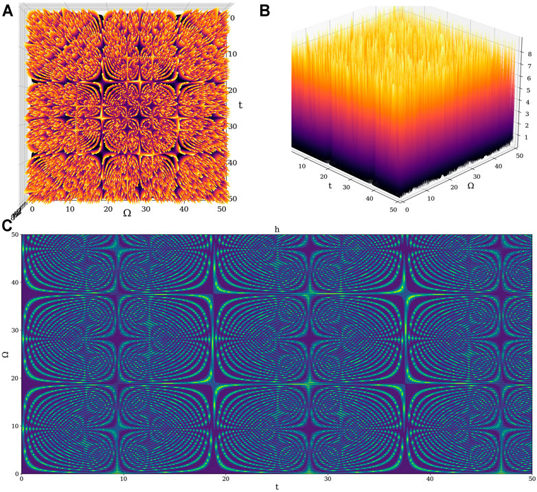
FIGURE 1. Example 3D plot of $h\left(\Omega ,t\right)$; (A) $\text{Φ}=2.35$, (B) (top, i.e., positive values); $\text{Φ}=2.35$ and (C) example 2D plot of $h\left(\Omega ,t\right)$; $\text{Φ}=2.35$.

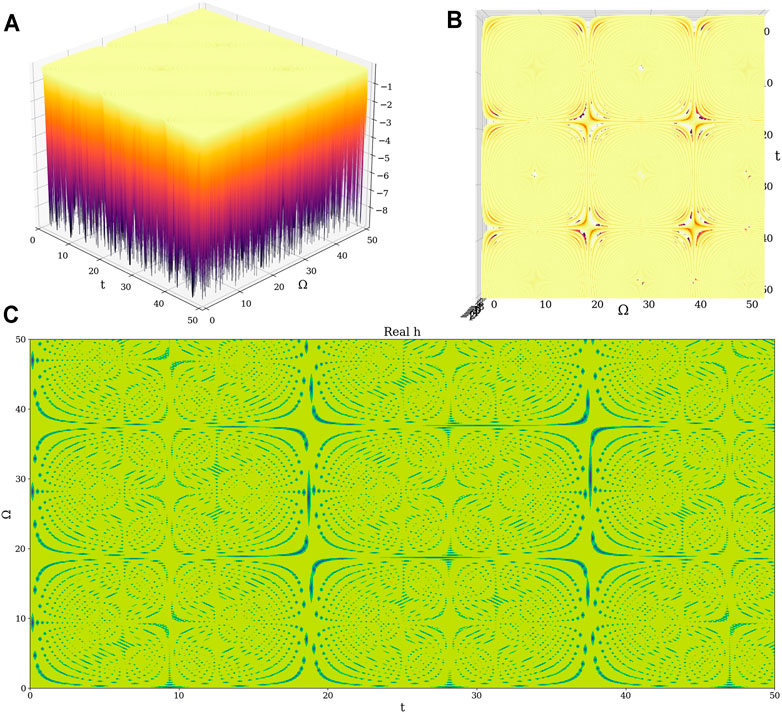
FIGURE 2. Example 3D plot of $Re\left[h\left(\Omega ,t\right)\right]$; (A) $\text{Φ}=2.35$, (B) (top, i.e., positive values); $\text{Φ}=2.35$ and (C) example 2D plot of $Re\left[h\left(\Omega ,t\right)\right]$; $\text{Φ}=2.35$.

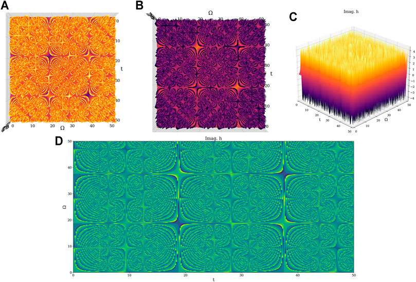
FIGURE 3. Example 3D plot of $Im\left[h\left(\Omega ,t\right)\right]$; (A) $\text{Φ}=2.35$, (B) (top, i.e., positive values); $\text{Φ}=2.35$, (C) (bottom, i.e., negative values); $\text{Φ}=2.35$ and (D) example 2D plot of $Im\left[h\left(\Omega ,t\right)\right]$; $\text{Φ}=2.35$.

Let us also note that the mathematical formalism of the Multifractal Theory of Motion naturally implies various operational procedures (invariance groups, harmonic mappings, groups isomorphism, embedding manifolds etc.) with quite a number of applications in complex systems dynamics (Agop and Merches, 2018; Mazilu et al., 2019). Interestingly, plotting $h$, once again in dimensionless parameters, also highlights certain temporal self-similar properties, with the multifractal structures being contained into similar multifractal structures at much higher scales (Figures 4A–C). This behavior is quite difficult to represent, because of the complicated balance between choosing an adequate number of plot points and manifesting self-similarity, but it shows how the small-scale behavior of the system ripples and $h$ manifests itself at higher scales, which is exactly what we would expect from a multifractal system. In order to reconfirm the presence of these behaviors, multiple other plots of this function have been performed in Mathematica through the Wolfram Alpha application (Figures 5A–D).

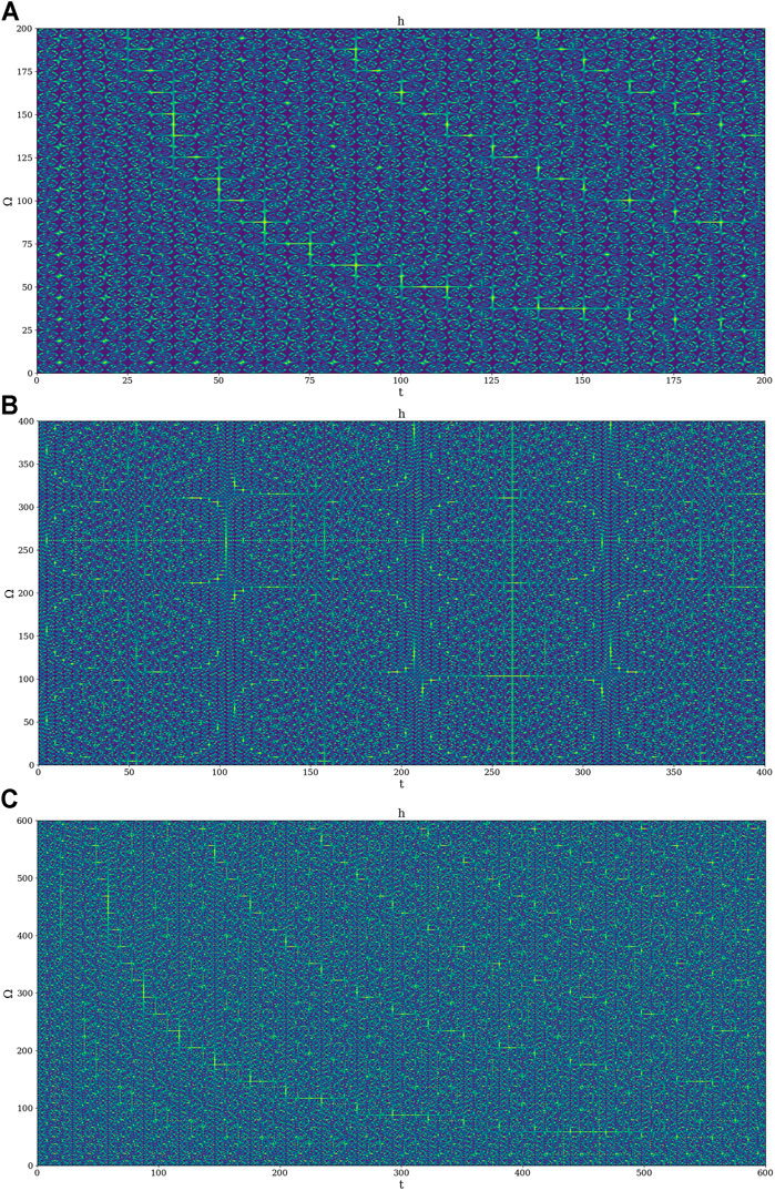
FIGURE 4. Example 2D plot of $h\left(\Omega ,t\right);$ (A) maximum at 200; $\text{Φ}=2.35$, (B) maximum at 400; $\text{Φ}=2.35$ and (C) maximum at 600; $\text{Φ}=2.35$.

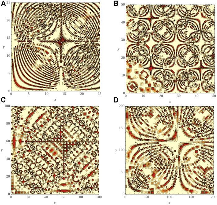
FIGURE 5. Example 2D plot of $h\left(\Omega ,t\right)$, in this case $x\equiv \Omega$, $y\equiv t$, in WolframAlpha; (A) maximum at 25; (B) maximum at 50, (C) maximum at 100, (D) maximum at 200.

The results presented in Figures 4, 5 also specify that, through self-structuring of atmospheric entities scale, transitions induced through the modification of fractal dimensions of movement curves that describe atmospheric dynamics can be assimilated to laminar channels. These channels are also described and observed in experimental data in our previous work (Roșu et al., 2021b).

Other nonlinear behaviors can be obtained by expanding the states density, the specific multifractal potential, and the multifractal non-differentiable velocity field. To this end, let us rewrite Eq. 22 based on Eq. 47, which produces:

In Figures 6A–C Eq. 48 is represented in dimensionless coordinates for a spontaneous symmetry break obtained through a Wick-type rotation in the hyperbolic plane (Ovchinnikov, 2016; Ovchinnikov et al., 2016; Hamilton, 2017). In such an operational procedure in dimensionless coordinates, $k$ found in Eq. 48 can be substituted with $\Omega$.

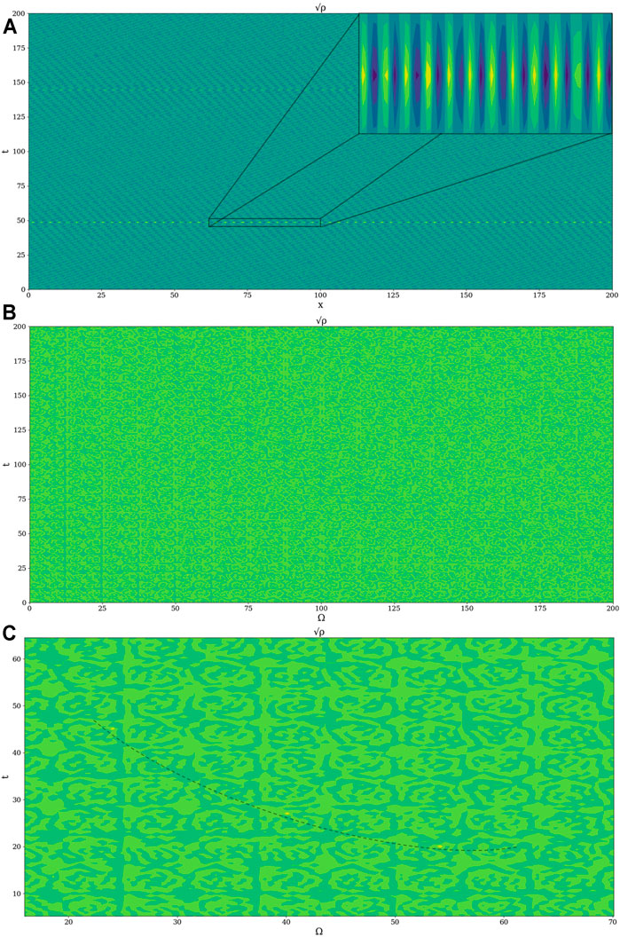
FIGURE 6. Example 2D plot of $\sqrt{\rho }\left(x,t\right)$; (A) zoom-in of multifractal synchronization modes (top-right); $\Omega =2.1$, $\text{Φ}=2.35$, (B) $x=5$, $\text{Φ}=2.35$, (C) zoomed-in region of $\sqrt{\rho }\left(\Omega ,t\right)$ multifractal synchronization modes; dotted line roughly shows synchronization modes distribution; $x=5$.$\text{Φ}=\mathrm{2.35.}$

Moving on to plots of other parameters of interest, the $\sqrt{\rho }\left(x,t\right)$ plot manifests multiple lines that represent synchronization modes at certain times; a sudden increase in activity throughout the length of the system of states density shows spontaneous “activations” of the multifractal entities leading to the increase of multifractal potential and of the potential appearance of multifractal force (Figure 6A). Multiple peaks are found throughout the figures plotted as a function of $\Omega$ and $t$ (Figure 6B). Notably, peaks in the $\sqrt{\rho }\left(\Omega ,t\right)$ plot seem to follow a pattern which corresponds to the appearance of the previously-described self-similarity (Figure 6C).

De aici, one can now calculate $Q$ and $V_F$ directly, slightly modifying previous equations to highlight $\Omega$, which implies, as previously-discussed:

The difference between the standard fluctuations of the plotted parameter fields and the spontaneous symmetry break peaks is too high in order to correctly show the orders of magnitude of each at the same time (Figures 7, 8). It must also be specified that these spontaneous symmetry break peaks are not calculus artefacts produced by point-wise derivation through Python code; the plots are drawn from analytically obtained functions.

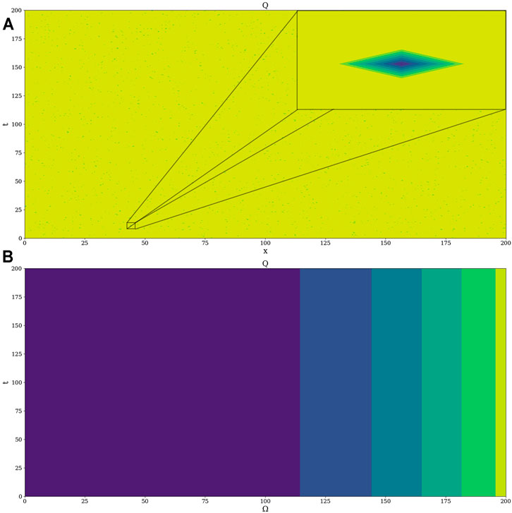
FIGURE 7. Example 2D plot of $Q\left(x,t\right)$; (A) zoom-in of spontaneous symmetry break peak (top-right); $\Omega =2.1$, $\text{Φ}=2.35$, (B) $x=5$, $\text{Φ}=2.35$.

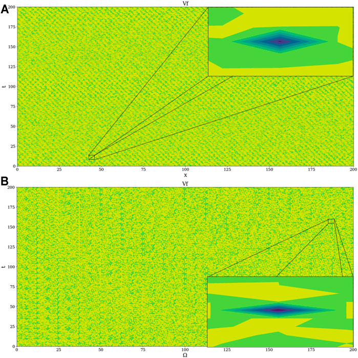
FIGURE 8. Example 2D plot of $V_F\left(x,t\right)$; (A) zoom-in of spontaneous symmetry break peak (top-right); $\Omega =2.1$, $\text{Φ}=2.35$, (B) zoom-in of spontaneous symmetry break peak (bottom-right); $x=5$, $\text{Φ}=2.35$.

The occurrence of anomalous, intense positive and negative peaks in the topology of our plots shows local spontaneous symmetry break for our equations corresponding to the $SL(2,R)$ group. This is because the appearance of the peaks violates the local symmetry of the equation fields, and these peaks also represent the spontaneous quality of the breaks because they appear even though the equations were developed under the assumption of laminarity. Now, in time-dependent dynamical systems, chaos is often described by the spontaneous break of topological symmetry, which is an intrinsic property of operators that describe all stochastic and deterministic differential equations (Ovchinnikov, 2016; Ovchinnikov et al., 2016). A local symmetry break might instead show that, at a given coordinate, time, and $\Omega$ parameter, peaks in the multifractal potential field might spontaneously appear. These peaks then represent variations and ripples in the potential field, which then shows the occurrence of multifractal forces spontaneously acting upon the multifractal laminar flow. Such forces do not immediately trigger chaos – in fact, the gradual occurrence of these forces can be responsible for the gradual development from laminar to chaotic flow according to the typical bifurcation sequence for the Navier-Stokes equations given by Ruelle and Takens, which is $steady\to periodic\to quasiperiodic\to chaotic$ (Reichl, 1992; McDonough et al., 2004). It must be highlighted that this standard route to chaos is also followed by the logistic map.

The objective now is to determine how and when these symmetry breaks occur, and this shall be done by checking the general variability of the potential at a varying $\Omega$. This can be shown by performing the bifurcation map of the inhomogeneity of $Q$. Now, in general, the total inhomogeneity of a parameter in a given volume $V$ of fluid is (Tatarski, 2016):

However, given our relatively limited spatial conditions, it shall suffice to consider the analysis of ${\left|Q\right|}^{\prime 2}$. Performing a Reynolds decomposition, it is possible to obtain (Alfonsi, 2009; Tatarski, 2016):

This parameter can then be iterated across $\Omega$ in a bifurcation map (Figure 9). The interpretation of these plots can be found in the following statements: for points given by $\Omega =2^n$, a general tendency towards stability is found, such that the inhomogeneity distribution is low and very concentrated (Figure 9). In fact, in these regions, the potential is always constant and equal to ${\Omega }^3$, such that $\left|Q\right|\left(x,t,\Omega =2^n\right)={\Omega }^3$ (Figure 9) – with a constant real potential, the implication is that the real multifractal force is null and there is a complete non-manifestation of any phenomena that might lead to turbulence of any kind. At the same time, regular variations in the $\sqrt{\rho }$ field are still present, which might indicate that a multifractal anti-synchronous behavior is taking place. Then, it is also possible to identify certain “mixture” areas; these manifest slightly higher average inhomogeneity, however inhomogeneity values are very widely spread out, pointing to uncertainty with regards to multifractal force generation. Finally, all other points show high and concentrated inhomogeneity – these signal areas of high potential for turbulence generation, and a significant amount of spontaneous local symmetry break peaks are guaranteed to be found in the multifractal potential field along with certain generation of multifractal force.

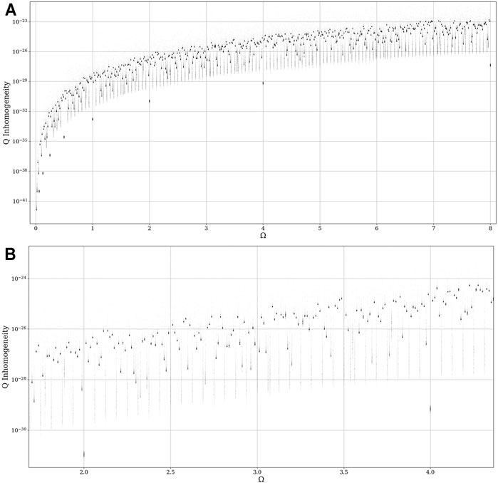
FIGURE 9. (A) Bifurcation diagram of ${\left|Q\right|}^{\prime 2}$, (B) Zoomed-in bifurcation diagram of ${\left|Q\right|}^{\prime 2}$.

Thus, there is a very clear and ordered intermittency between homogeneity, inhomogeneity, and “mixture” states, and it is this behavior that gives rise to the gradual process of turbulent energy cascades. All throughout this analysis, it is important to remember that the bifurcation maps show the “potentiality of turbulence” of a given flow at a given point as $\Omega$ increases, given the fact that the equations were developed on the premise of laminarity. Furthermore, these points of stability in the potential bifurcation maps cannot exactly show the spatio-temporal coordinates of the spontaneous symmetry breaks because of the averaging in the inhomogeneity calculation (Eq. 54); for this, it is necessary to plot individual samples of inhomogeneity. On the other hand, it is significant that the dependency $\left|Q\right|\left(x,t,\Omega =2^n\right)={\Omega }^3$, in terms of the stability behavior found at the doubling of $\Omega$, is similar to scale variation and vortex bifurcating behavior exhibited by a different model.

In our previous works, we have made use of a modified $\beta$-constant turbulence cascade scale model, developing it in relation to lidar data (Roșu et al., 2020; Roșu et al., 2021a). The typical gauge employed by such models is a dependency of type:

Given the fact that $\Omega$ is intrinsically connected to the scale resolution, it is only natural that similarities between this model and our current results are found; it would then be helpful to determine whether or not the $\beta$-constant model can show whether or not a ${\Omega }^3$-type relation might occur in terms of a diffusion coefficient of the modelled flow. However, according to the equations found through developing this model in our previous works, both molecular and turbulent diffusion parameters are constant throughout the flow; this takes place because the scale resolution is taken to be constant (Roșu et al., 2021b). Fundamentally, the $\beta$-constant turbulence cascade scale model is inadequate because of the scale resolution non-variability in the $2^{n{\left(dt\right)}^2}$ term which describes scale progression in this case. Instead, if the scale resolution is not constant, not only would these parameters be variable, but it would be possible to obtain not just a variable fractal dimension but also a proper multifractal singularity spectrum $f\left(\alpha \right)$ as required here.

In our previous study, a similar conclusion regarding the $\beta$-constant model was reached regarding connecting it to the logistic map – because fitting this model to the map would yield unequal scale ratios, which goes against the principle of a $\beta$-constant which implies that such scale and volume ratios remain constant throughout the turbulent energy cascades. It seems that both the bifurcation diagram of the logistic map and the inhomogeneity evolution have similar properties. Furthermore, in a previous study it has been shown that it is possible to reduce velocity modes of a multifractal Navier-Stokes equation to the logistic map, pointing to the existence of such a connection (Roșu et al., 2020; Roșu et al., 2021a; Roșu et al., 2021b). We propose that the non-manifest scenario of chaos shown by the bifurcation diagram of multifractal potential inhomogeneity generally describes both non-chaotic intervals in such maps used to model atmospheric flow, and also potential chaos arising from spontaneous symmetry breaks in the parameter fields describing such flows.

In order to better illustrate the potential origin of this quasi-periodic and intermittent character of the inhomogeneity of the multifractal potential, it is possible to rewrite $\sqrt{\rho }$ such that it is a function of $r$, $\Omega$ and $t$ with the last two parameters fully contained in simple trigonometric functions. We start with:

This can then be considered as:

with:

which results in:

This function has been plotted in Figure 10. In itself, the simple trigonometric function $\cos \left(xy\right)$ is subject to numerous interesting behaviors, including cellular structures and topological instabilities; as such, its presence in the function of the multifractal velocity state density function, which is then used to calculate the specific multifractal potential, could be what points to cellular structures and the symmetry breaking peaks. In fact, most simple trigonometric functions containing two or more multiplied independent parameters seem to exhibit complex, quasi-periodic and even fractal behavior at higher values of the given parameters. In any case, $\cos \left(xy\right)$ can be difficult to describe as a function of simpler trigonometric functions, except by using Chebyshev polynomials which presuppose that $x$ or $y$, in this case $\Omega$ or $t$, has a positive integer value (Mason and Handscomb, 2002).

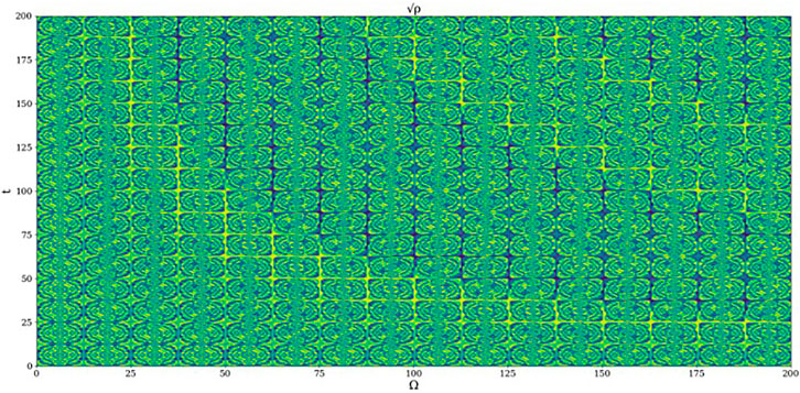
FIGURE 10. Example 2D plot of the alternative equation of $\sqrt{\rho }\left(\Omega ,t\right)$; $x=5$, $\text{Φ}=2.35$.

In terms of the theory presented here, our results clearly suggest that the transition from laminar to chaotic might come from spontaneous sources; the opposite is also true, given the correspondence between the logistic map and the Navier-Stokes equation and the sudden intervals of stability found in the logistic map throughout the Pomeau-Manneville area. This then suggests that there exist laminar channels throughout the atmosphere – not only that, but the cellular linear entities found in $h$ heavily imply that such laminar areas self-structure themselves in cohesive and coherent ways across space. Furthermore, in a previous study, such channels have been found to exist in the atmosphere through experimental lidar data; their existence and characteristics can be demonstrated and analyzed again through novel sets of data. In the following figures, this is done by first presenting the Range Corrected Signal (RCS) timeseries plot (Figure 11), then the corresponding analysis of these signals is performed by calculating vortex length scales using the signals. For these, by associating a modified turbulence cascade model to the logistic map as per an earlier study, a corresponding $r$ value is obtained, which is then used to obtain a corresponding maximal Lyapunov exponent (Roșu et al., 2021b). These exponents can then be used to quantify chaoticity at a given stage of the turbulent cascade at a given altitude, and it is indeed found that segments of the analyzed atmospheric flow are not chaotic at all (Figure 12).

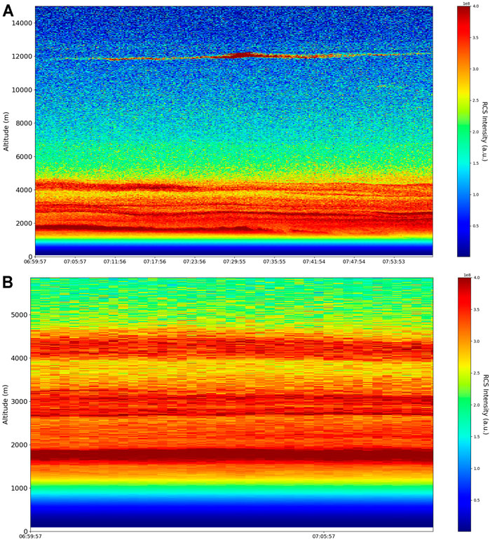
FIGURE 11. (A) RCS timeseries, Bucharest, Romania, 13/06/2019, (B) zoomed RCS timeseries, Bucharest, Romania, 13/06/2019; area of interest for subsequent laminar channel study.

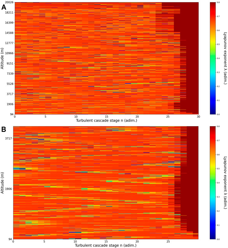
FIGURE 12. (A) Lyapunov exponent per turbulent cascade stage colormap altitude plot, Bucharest, Romania, 13/06/2019, 07:00:00, (B) zoomed-in Lyapunov exponent per turbulent cascade stage colormap altitude plot, Bucharest, Romania, 13/06/2019, 07:00:00.

The RCS data used in this study has been obtained from the RALI Multiwavelength Raman Lidar Platform, which is a part of the National Institute for Research and Development in Optoelectronics INOE 2000 in Bucharest, Romania, 93 $m$ ASL (Figure 11). The laser emission wavelengths are $1064nm$ ($90mJ$), $532nm$ ($50mJ$) and $355nm$ ($60mJ$) and the detection channels are $1064$, $532$ cross, $532$ parallel, $355nm$ (elastic wavelengths), and $607$, $387$ and $408nm$ (Raman channels). A $532nm$ set has been used for this study (Figure 11). The laser pulse duration is $7-9ns$, repetition rate $10Hz$, and the beam diameter between $5.5-7mm$ at FWHM. The dynamic range covers $2-15km$ depending on atmosphere transmission, with a $3.75m$ spatial resolution. The reception has a $400mm$ Cassegrain telescope with $1.73mrad$ field of view, and the system acquisition is both analog and photon counting, with a $20MS/s$ analog sampling rate and $250Mhz$ photon counting count rate. The RALI lidar system was upgraded and tested against other lidar systems, and its results have been published in multiple other studies (Belegante et al., 2018; Nicolae et al., 2018; Adam et al., 2020).

Regarding the obtained RCS data, many features of the atmosphere can be directly observed in what appears to be a calm, typical atmospheric scenario, including but not limited to stratospheric cirrus clouds, pollutant plumes and the PBL – it possible to confidently exclude the presence of clouds in the lower atmosphere, given the fact that Meteomanz.com displays clear conditions for the “Bucuresti Filaret” station, which happens to be closest to the lidar platform, and also given the fact that ACTRIS lidar data collecting procedure demands that data collecting start only during clear conditions (Figure 11). In relation to the laminar analysis, certain “V-shaped structures” can be observed; these are the laminar channels, and their presence is given by the fact that, at a certain altitude, the inequality necessary for laminar behavior is satisfied, and then satisfied again at a different altitude at a different or similar scale (Figure 12). We thus identify “ascending” or “descending” laminar channels, and these structures can help explain various atmospheric transport phenomena regarding aerosols and cloud formations, but also regarding PBL stability (Figure 12). The classification difference between “ascending” and “descending” is justified by the fact that the turbulent cascade progresses from larger to smaller scales; thus, it is necessary to assume that a continuation of the laminar channel at higher altitude towards smaller scales indicates, for example, that the channel is ascendent.

Conclusion

In this study, we have found that representing laminar atmospheric flows in a multifractal framework reveals unexpected results that might explain emergent turbulent behavior. Even by approaching these equations from an irrotational perspective, it is shown that relations between them and the $SL(2,R)$ symmetry group lead to self-structuring cellular structures in the multifractal velocity field and to a fluctuating multifractal specific potential field. These fluctuations take the form of peaks which represent local spontaneous symmetry breaks in the topology of the potential field, being singularities that lead to turbulence generation. This then indicates that the laminar multifractal flow is spontaneously subjected to occurrences of multifractal force at a given position and time, and these forces might lead to the intermittency and quasi-periodicity commonly associated with the transition to turbulent flow. Furthermore, a regularity relation exists which shows periods of stability and instability in the potential field, as shown by the evolution of the inhomogeneity of this potential field, and this evolution can be connected to the logistic map, which itself can be roughly connected to the Navier-Stokes equation as seen in multiple other studies. The self-structuring cellular aspect of the multifractal flow is otherwise found to be connected to exotic behaviors of simpler functions. Finally, the emergence relations between laminarity and turbulence imply the existence of what have been named “laminar channels” in a previous study, and the connection between theory and experiment is made by highlighting such laminar structures in atmospheric lidar data. Further experimentation will be necessary in order to better quantify these relations and to develop methods of using them in a predictive scenario, in the context of both meteorology and atmospheric science in general.

Data Availability Statement

The raw data supporting the conclusions of this article will be made available by the authors, without undue reservation.

Author Contributions

Conceptualization, I-AR, MC, D-CN, and MA; methodology, I-AR and MA; software, I-AR; validation, I-AR, MC, D-CN, and MA; formal analysis, I-AR, MC, D-CN, and MA; investigation, I-AR, MC, D-CN, and MA; resources, I-AR, D-CN, and MC; data curation, I-AR, MC, and MA; writing—original draft preparation, I-AR, MC, D-CN, and MA; writing—review and editing, I-AR, MC, D-CN, and MA; visualization, I-AR, MC, D-CN, and MA; supervision, MA and D-CN; project administration, I-AR, MC, D-CN, and MA; funding acquisition, I-A.R, D-CN, and MC. All authors have read and agreed to the published version of the manuscript.

Funding

This work was supported by a grant from the Romanian Ministry of Education and Research, CNCS-UEFISCDI, project number PN-III-P1-1.1-TE-2019-1921, within PNCDI III.

Conflict of Interest

The authors declare that the research was conducted in the absence of any commercial or financial relationships that could be construed as a potential conflict of interest.

Publisher’s Note

All claims expressed in this article are solely those of the authors and do not necessarily represent those of their affiliated organizations, or those of the publisher, the editors and the reviewers. Any product that may be evaluated in this article, orclaim that may be made by its manufacturer, is not guaranteed or endorsed by the publisher.

Acknowledgments

The authors acknowledge the RADO (Romanian Atmospheric 3D research Observatory) and ACTRIS – RO (Aerosol, Clouds and Trace gases Research InfraStructure - Romania) for providing the lidar data used in this study. They also acknowledge the Faculty of Geography and Geology of the “Alexandru Ioan Cuza” University of Iaşi for the financial support offered for the publication of this study.

References

Adam, M., Nicolae, D., Stachlewska, I. S., Papayannis, A., and Balis, D. (2020). Biomass burning events measured by lidars in EARLINET - Part 1: Data analysis methodology. Atmos. Chem. Phys., 20, 13905–13927. doi:10.5194/acp-20-13905-2020
Agop, M., and Mazilu, N. (2011). Skyrmions: A Great Finishing Touch to Classical Newtonian Philosophy. New York, NY: Nova Science Publisher. Available at: https://www.researchgate.net/publication/287262893_Skyrmions_A_great_finishing_touch_to_classical_newtonian_philosophy.
Agop, M., and Merches, I. (2018). Operational Procedures Describing Physical Systems. CRC Press, Boca Raton, Florida.
Agop, M., and Paun, P. V. (2017). On the New Perspective of Fractal Theory. Fundaments and Applications; Editura Academiei Romane, București, Romania.
Alfonsi, G. (2009). Reynolds-averaged Navier–Stokes Equations for Turbulence Modeling, Appl. Mech. Rev., 62, 040802 (20 pages). doi:10.1115/1.3124648
Belegante, L., Bravo-Aranda, J. A., Freudenthaler, V., Nicolae, D., Nemuc, A., and Ene, D.(2018). Experimental Techniques for the Calibration of Lidar Depolarization Channels in EARLINET. Atmos. Meas. Tech., 11(2), 1119–1141. doi:10.5194/amt-11-1119-2018
Cristescu, C. P. (2008). Nonlinear Dynamics and Chaos. Theoretical Fundaments and Applications. Bucharest: Romanian Academy Publishing House, Bucharest, Romania.
Hamilton, M. J. (2017). Mathematical Gauge Theory. Springer International Publishing AG, New York US.
Jaynes, E. T. (1973). The Well-Posed Problem. Foundations Phys., 3(4), 477–493. doi:10.1007/bf00709116
Mandelbrot, B. B. (1982). The Fractal Geometry of Nature; W. H. Freeman: San Fracisco, CA, USA, pp. 80–103.
Mazilu, N., Agop, M., and Mercheş, I. (2019). The Mathematical Principles of Scale Relativity Physics: The Concept of Interpretation. CRC Press, Boca Raton, Florida.
McDonough, J. M., and Huang, M. T. (2004). A ‘poor Man's Navier–Stokes Equation’: Derivation and Numerical Experiments—The 2‐D Case. Int. J. Numer. Methods Fluids, 44(5), 545–578. doi:10.1002/fld.657
Merches, I., and Agop, M. (2015). Differentiability and Fractality in Dynamics of Physical Systems. World Scientific, Singapore.
Mihaileanu, N. (1972). Geometrie analitica, proiectiva si diferentiala. Complemente, Ed. Didactica si Pedagogica, Bucharest, 3.
Nicolae, D., Vasilescu, J., Talianu, C., Binietoglou, I., Nicolae, V., Andrei, S., et al. (2018). A Neural Network Aerosol-Typing Algorithm Based on Lidar Data. Atmos. Chem. Phys., 18(19), 14511–14537. doi:10.5194/acp-18-14511-2018
Nottale, L. (2011). Scale Relativity and Fractal Space-Time: A New Approach to Unifying Relativity and Quantum Mechanics. Imperial College Press: London, UK, pp. 403–425.
Ovchinnikov, I. V. (2016). Introduction to Supersymmetric Theory of Stochastics. Entropy, 18(4), 108.doi:10.3390/e18040108
Ovchinnikov, I. V., Schwartz, R. N., and Wang, K. L. (2016). Topological Supersymmetry Breaking: The Definition and Stochastic Generalization of Chaos and the Limit of Applicability of Statistics. Mod. Phys. Lett. B, 30(08), 1650086.doi:10.1142/s021798491650086x
Roşu, I. A., Cazacu, M. M., Ghenadi, A. S., Bibire, L., and Agop, M. (2020). On a Multifractal Approach of Turbulent Atmosphere Dynamics. Front. Earth Sci., 8, 216. doi:10.3389/feart.2020.00216
Roşu, I. A., Cazacu, M. M., and Agop, M. (2021a). Multifractal Model of Atmospheric Turbulence Applied to Elastic Lidar Data. Atmosphere, 12(2), 226. doi:10.3390/atmos12020226
Roşu, I. A., Nica, D. C., Cazacu, M. M., and Agop, M. (2021b). Towards Possible Laminar Channels through Turbulent Atmospheres in a Multifractal Paradigm. Atmosphere, 12(8), 1038. doi:10.3390/atmos12081038
Sors, L. A. S., and Santaló, L. A. (2004). Integral Geometry and Geometric Probability. Cambridge University Press, Cambridge, England.
Tatarski, V. I. (2016). Wave Propagation in a Turbulent Medium. Courier Dover Publications, Mineola, New York, US.
Keywords: self-structuring, turbulent (channel) flow, laminar channel flow, atmosphere, multifractal, LIDAR - remote sensing
Citation: Roșu I-A, Nica D-C, Cazacu MM and Agop M (2022) Cellular Self-Structuring and Turbulent Behaviors in Atmospheric Laminar Channels. Front. Earth Sci. 9:801020. doi: 10.3389/feart.2021.801020
Received: 24 October 2021; Accepted: 14 December 2021;
Published: 21 January 2022.
Edited by:
Iuliana Oprea, Colorado State University, United StatesReviewed by:
Eugen Radu, University of Aveiro, PortugalLeila Marek Crnjac, Technical School Centre Maribor, Slovenia
Copyright © 2022 Roșu, Nica, Cazacu and Agop. This is an open-access article distributed under the terms of the Creative Commons Attribution License (CC BY). The use, distribution or reproduction in other forums is permitted, provided the original author(s) and the copyright owner(s) are credited and that the original publication in this journal is cited, in accordance with accepted academic practice. No use, distribution or reproduction is permitted which does not comply with these terms.
*Correspondence: Dragos-Constantin Nica, dragos.nica@uaic.ro; Marius Mihai Cazacu, cazacumarius@gmail.com