Mixed Integration Scheme for Embedded Discontinuous Interfaces by Extended Finite Element Method

Introduction

The extended Finite Element Method (XFEM) is an excellent numerical method that can visually simulate discontinuous cracks/interfaces and their evolution without mesh regeneration. By introducing enrichment functions with special local properties into the partition of unit method (PUM) framework, this method can enable construction of discontinuous fields within local elements (Belytschko and Black, 1999; Moës et al., 1999; Belytschko et al., 2001). As it offers several advantages, XFEM has been applied to failure problems in many different fields, including geotechnical and geological engineering (Abdelaziz and Hamounie, 2008; Belytschko et al., 2009; Fries and Belytschko, 2010; Gracie and Graig, 2010; Salimzadeh and Khalili, 2015; Matthew and Caglar, 2016; Li et al., 2018; Wang et al., 2018; Cruz et al., 2019). It can be predicted that XFEM will play a more important role in the modeling, assessing, and preventing of geotechnical and geological disasters. However, the wider application of XFEM is limited by several drawbacks. One of these drawbacks is that with the introduction of discontinuous functions, standard Gaussian integration cannot be applied directly to XFEM-enriched elements, and splitting of elements into subcells is often necessary. XFEM converts the complexity of mesh regeneration into the complexity of the discontinuous function integration within the element (Chin et al., 2017). Another drawback is that due to the same interpolation basis functions used, the enriched degrees of freedom (DOFs) of a node may become almost linearly dependent on the regular DOFs of the node, leading to ill-conditioned system equations. The nearly linear dependency and ill-conditioning are especially apparent for discontinuous enrichment functions when the interface approaches an element node and crack tip singular enrichment functions at a certain distance from the singular point (Sukumar et al., 2015; Ventura and Tessei, 2016; Agathos et al., 2019).

Generally, integrating the weak form within an element with discontinuous interfaces requires element splitting. This approach has strong adaptability and has been widely used in previous studies (Moës et al., 1999; Belytschko et al., 2001; Belytschko et al., 2009; Fries and Belytschko, 2010; Li et al., 2018). However, implementation of the element-splitting algorithm is complicated and not uniform. Additionally, it presents challenges concerning the integration point mapping in nonlinear constitutive models. Studies have been devoted to the integration of non-polynomial enrichment functions (discontinuous functions or singular functions) without element splitting. The representative methods include the equivalent polynomial integration method (Ventura 2006; Ventura and Benvenuti, 2015), the arbitrary polygon integration method (Natarajan et al., 2009; Natarajan et al., 2010), the arbitrary domain integration method (Joulaian et al., 2016), and the Legendre polynomial equivalent integration method (Abedian and Düster, 2019), et al. At present, these methods are usually limited to two-dimensional (2-D) conditions; three-dimensional (3-D) implementations remain a challenge. In addition, these methods cannot address curved or kinked cracks/interfaces within an element. Song et al. (2006) used a partition ratio-weighted single-point reduced integration to integrate the weak form of quadrilateral elements with discontinuous enrichment functions, thereby avoiding element splitting and historical variable mapping. However, single-point reduced integration is equivalent to assuming that the element is constantly strained, which results in poor solution accuracy (Wang et al., 2021).

For unstructured meshes and arbitrary non-planar cracks/interfaces, cases with cracks/interfaces close to element nodes are inevitable, which lead to ill-conditioned system equations. Previous approaches for solving this problem include directly removing the enrichment of nodes whose enrichment functions have only small supports in the cut element (Daux et al., 2000; Bordas et al., 2007), and adjusting the node coordinates such that the partition ratio is not unreasonably small (Choi et al., 2012). However, the former approach introduces interpolation errors, while the latter is not a generalizable method, especially for 3-D problems. Reusken (2008) proposed a method to impose constraints on the enriched DOFs with a small partition ratio, limiting its value to zero; this is essentially the same as removing the enrichment. Ventura and Tesei (2016) proposed a stabilized method that imposes constraints on the enriched DOFs through a penalty method, reducing the additional error caused by the constraints. Other studies have adopted the approach of preconditioning the ill-conditioned system equations to improve convergence. For example, Sauerland and Fries (2013) studied the Jacobi preconditioner, and Béchet et al. (2005) developed a preconditioner based on Cholesky decomposition. However, this approach becomes cumbersome for nonlinear problems and crack evolution problems because the Jacobian matrix must be re-preconditioned after each update, which significantly increases the amount of calculation.

Based on the research of Song et al. (2006), the partition ratio-weighted integration method was improved in this study and is referred to as “smeared” integration method. It was observed that this method could significantly alleviate the ill-conditioning caused by the nearly linear dependence of DOFs enriched by the discontinuous functions. Furthermore, this method (for the integration of the Jacobian matrix) was combined with the subcell (element splitting) integration method (for the integration of residuals) to produce a mixed integration scheme, which not only resulted in well-conditioned system equations but also ensured a high solution accuracy.

The remainder of this paper is structured as follows: Firstly, the XFEM formulation is sketched out, and the weak form of the equilibrium equation is presented, including the interface contact relationship and the integral form of the Jacobian matrix. Secondly, the smeared integration method is presented, and its performance is demonstrated through a series of element analyses. Then, the mixed integration scheme is proposed and verification is made in the next section through two benchmark examples. Finally, the main conclusions of this study are summarized in the last section of this paper.

XFEM Formulation

Strong and Weak Form of Boundary Value Problem

A quasi-static boundary value problem with internal interfaces was assumed, as shown in Figure 1. In the solution domain $\text{Ω}$, there exists a strong discontinuous interface ${\text{Γ}}_d$, the two sides of which are denoted as ${\text{Γ}}_d^{+}$ and ${\text{Γ}}_d^{-}$; the corresponding normal vectors are ${\mathit{n}}^{+}$ and ${\mathit{n}}^{-}$, respectively. $\mathit{b}$ is the body force in the domain; ${\text{Γ}}_t$ is the force boundary, and ${\text{Γ}}_u$ is the displacement boundary.

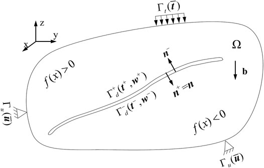
FIGURE 1. Diagram of boundary value problem with crack.

The force equilibrium conditions must be satisfied in the continuum, and the corresponding Dirichlet or Neumann boundary conditions must be satisfied at the boundaries. Thus, the governing equations of the boundary value problem are

Contact forces ${\mathit{t}}^{+}$ and ${\mathit{t}}^{-}$ are defined on the internal interfaces ${\text{Γ}}_d^{+}$ and ${\text{Γ}}_d^{-}$, respectively. They satisfy the equilibrium condition and can be expressed as a unified variable:

${\mathit{u}}^{+}={\mathit{u}|}_{{\mathrm{\Gamma }}_d^{+}}$ and ${\mathit{u}}^{-}={\mathit{u}|}_{{\mathrm{\Gamma }}_d^{-}}$ correspond to the displacement vectors on the two sides of the internal interface; the relative displacement on the interface is defined as

The kinematics admissible (trial) space and the weighting (test) space of the displacement are defined as

For $\mathit{u}\left(\mathit{x}\right)\in \mathcal{U}$ and any $\delta \mathit{u}\left(\mathit{x}\right)\in {\mathcal{U}}_0$, the equivalent integral weak form of the governing equations can be expressed as

where $\delta W^{int}$, $\delta W^{\mathrm{ext}}$, and $\delta W^c$ are the work of the internal force, external force, and interface contact force, respectively, and are expressed as

where ${\mathit{\nabla }}_s$ is the symmetric gradient operator.

According to the definitions of t (Eq. 2) and w (Eq. 3), the expression of $\delta W^c$ in Eq. 7 can be simplified as

The constitutive relationship of the continuum is expressed as

where D is the constitutive tensor. The traction-displacement relationship of the interface can also be expressed in a constitutive form as

where ${\mathit{D}}^{\Gamma }$ is the interface constitutive tensor, implemented by imposing constraints on the interface in practice; Q is the transfer matrix from local coordinates to global coordinates.

Discretization and Jacobian Matrix

For simplicity, only a case with elements completely separated by the interface was considered, and only the Heaviside enrichment function was used in this study. Nevertheless, the conclusions of this study also hold for a case that the end of the interface stays inside the element, for which treatments have been provided by Zi and Belytschko (2003), Kumar and Bhardwaj (2018).

The displacement approximation in a shifted form is expressed as

where the first summation term represents the standard FE approximation, and the second summation term represents the XFEM-enriched discontinuous approximation; I is the set of all nodes in the discrete domain; I*∈I is the set of enriched nodes; $N_i$ is the regular finite element basis function of node i; ${\mathit{u}}_i$ and ${\mathit{q}}_i$ are the regular DOF vector and the enriched DOF vector of node i, respectively; and $H$ is the Heaviside enrichment function, which is expressed as

where $f\left(\mathit{x}\right)$ is a signed distance function depending on the definition of the positive normal of the discontinuous interface, as shown in Figure 1.

Considering the variation in the discrete approximation of the displacement field given by Eq. 11, the testing field can be obtained:

According to the definition of the interface relative displacement w given by Eq. 3, the continuous term of the displacement field has no contribution to w; instead, w is determined by the discontinuous term, as follows:

Its variational form is expressed as

By substituting the testing fields expressed in Eqs 13, 15 into the equivalent integral weak form of Eq. 6, and considering the arbitrary nature of these fields, the following discrete form of the equilibrium equations can be obtained:

where ${\mathit{f}}_u^{\mathrm{int}}$ and ${\mathit{f}}_u^{\mathrm{ext}}$ are the nodal internal force vector and nodal external force vector, respectively, corresponding to the regular DOFs; ${\mathit{f}}_q^{\mathit{int}}$ and ${\mathit{f}}_q^{ext}$ are the nodal internal force vector and nodal external force vector, respectively, corresponding to the enriched DOFs; and ${\mathbf{f}}^c$ is the nodal interface contact force vector. All these vectors are integrated from the nodal force vectors of related elements, and their specific expressions are presented in Eq. 17:

where B is the discrete strain–displacement operator, and H and H_I are the matrix forms of the Heaviside function and its nodal values, respectively.

Taking the derivative of Eq. 16 with respect to the displacement fields and considering Eq. 17, the Jacobian (stiffness) matrix of the finite element discretization equations can be obtained as

where

When the same basis function is used, the Jacobian matrix expressed as Eq. 18 may have a large condition number, especially when the interface is close to the enriched nodes. Thus, the enriched DOFs and the standard DOFs are almost linearly dependent, and the matrix tends to be severely ill-conditioned.

Smeared Integration Method and Mixed Integration Scheme

Smeared Integration Method

Based on Eqs 12, 19 and considering H² = H, the numerical integration of the discontinuous part (multiplied with the Heaviside function) for each term in the stiffness matrix can be generalized in the following form:

where $p\left(x\right)$ is an arbitrary polynomial function. Evidently, the discontinuity in the integrand arises from the discontinuity in $H\left(x\right)$.

As shown in Figure 2, a directional interface cut the element into two subdomains ${\text{Ω}}_A$ and ${\text{Ω}}_B$, denoting the positive and negative parts of the signed distance function, respectively. The integration of the discontinuous function over the entire element is converted to a summation of continuous function integrations over the two subdomains [$H\left(x\right)$ is constant on each side]:

Noted that $H\left(x\right)$ equals to unit on ${\text{Ω}}_A$ and vanishes on ${\text{Ω}}_B$, Eq. 20 can be simplified as

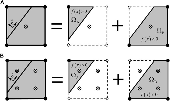
FIGURE 2. Diagram of integration of element cut by a discontinuous interface (with a 2-D quadrilateral element as an example). (A) Integration method proposed by Song et al. (2006). (B) Smeared integration method.

As the subdomains can be arbitrary polygons, the calculation of Eq. 22 often requires further division of the subdomains into triangular subcells, as illustrated in Figure 3, which brings much burden for calculation.

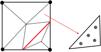
FIGURE 3. Diagram of subcell integration of element cut by discontinuous interface (with a 2-D quadrilateral element as an example).

To avoid element decomposition, Song et al. (2006) integrated Eq. 20 over the entire element domain via single-point reduced integration with hourglass control. Their starting point was the assumption that all elements are constant-strain elements [p(x) = C]; thus, the integration over the subdomain could be replaced with integration over the entire element domain with a coefficient representing the subdomain contribution:

where R is the partition ratio of the element cut by the interface and is defined as

Clearly, R is related to the location and configuration of the interface; thus, it can reflect the distribution characteristics of the discontinuous function defined on the element to some extent. The rightmost integral in Eq. 23 is performed over the entire element domain; thus, standard Gaussian integration can be performed directly. However, the assumption of constant-strain elements reduces the integration accuracy and prevents an accurate reflection of the constitutive behaviors of nonlinear materials.

Based on the method of Song et al. (2006), single-point reduced integration was replaced with quadratic Gaussian integration in this study, as shown in Figure 2B. This alteration obviated the constant-strain assumption and the need for hourglass control. The integral domain remained unchanged, and the influence of $H\left(x\right)$ was reflected approximately by R:

This integration method is simple and can be easily implemented. The integration points remain consistent before and after the discontinuity interface is introduced; thus, no historical variable mapping is required. However, this method ignores the shape information of the real integration domain and introduces information from the integrand function outside the domain. This approach is similar to a smearing/homogenizing operation; it can be referred to as “smeared” integration and is expressed as

Although this method suffers from certain approximation errors, it offers several advantages: (i) Compared with subcell integration, the smeared integration method avoids element splitting and significantly reduces the number of required integration points. (ii) In each element, the Gaussian integration of ${\mathit{B}}^T\mathit{DB}$ needs to be performed only once. Only ${\mathit{K}}_{uu}$ in Eq. 19 must be integrated; while the integration of ${\mathit{K}}_{uq}$ and ${\mathit{K}}_{qq}$ can be achieved by multiplying ${\mathit{K}}_{uu}$ with corresponding coefficients related to the partition ratio R, which further reduces the calculation complexity. The detailed relations between these matrixes are derived in the Supplementary Appendix. (iii) The stiffness matrix conditions are improved, and the nonlinear iteration stability is enhanced. These features are demonstrated in detail in the following sections.

Error Analysis of Smeared Integration

If the continuous integrand $p\left(x\right)$ is a constant, the smeared integration is accurate, as expressed in Eq. 23. If $p\left(x\right)$ is a linear or higher-order polynomial, the smeared integration has a certain approximation error that is, directly related to the order of $p\left(x\right)$ and the location of the discontinuous interface relative to the element (represented by the partition ratio R).

Defining the approximation error of the smeared integration (Eq. 25) by comparing with the exact discontinuous function integration (Eq. 21):

For low-order continuous integrand $p\left(x\right)$, there exists a point $x_i$ in the domain ${\text{Ω}}_A$, satisfying:

Similarly, there exists a point $x_j$ in the domain ${\text{Ω}}_{\text{B}}$, satisfying:

Where S_A and S_B are the areas of ${\text{Ω}}_A$ and ${\text{Ω}}_{\text{B}}$, respectively.

Noted that, S_A = R∗S, S_B = (1-R)*S, where S is the area of the intact element $\text{Ω}$, Eq. 27 can be rewritten as:

Several conclusions can be drawn from this expression:

(i) For a fixed partition ratio R, a higher order of $p\left(x\right)$ produces a greater difference between $p\left(x_i\right)$ and $p\left(x_j\right)$, thus greater approximation error in the smeared integration. Order of $p\left(x\right)$ decides the upper bound of the error. For the bilinear/trilinear elements used in this study, the errors were limited and were influenced more strongly by the location of the interface.

(ii) R behaves as a scale factor of the error. When $R\to 0$ or $R\to 1$, the error approaches zero with the same order with R or 1-R. Actually, these two conditions are equivalent as they are interconvertible by changing the definition of the interface direction in Figure 2.

(iii) When $R\to 0.5$, the smeared integration has a relatively large error because the shape information of the real integration domain is ignored. For the three cases illustrated in Figure 4, the same stiffness matrix is calculated from the smeared integration; thus, smeared integration is not recommended in this condition.

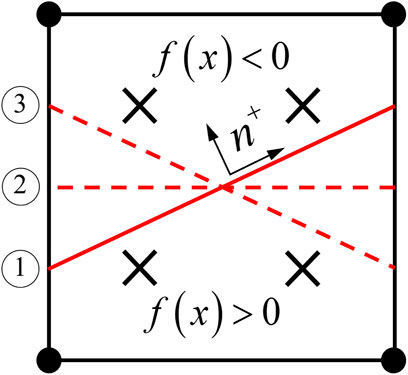
FIGURE 4. Diagram of case where “smeared integration” method is not recommended.

Influence of Smeared Integration on Element Stiffness Condition

To understand the effects of partition ratio R and the configuration of the discontinuous interface on the efficacy of smeared integration, element tests for four typical cases, as shown in Figure 5¹, were performed. The element stiffness matrices were calculated via subcell integration and smeared integration. The square element has a side length of a = 1 and an elastic modulus of E = 1.0. Only four integration points are required for each cracked element by the smeared integration while the subcell integration involved the third-order Hammer integration with four integration points in each triangle subcell.

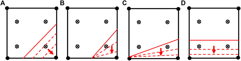
FIGURE 5. Diagram of typical partition patterns of discontinuous interface: (A) Interface cuts adjacent sides of element, cutting angle fixed at 45°; (B) Interface cuts adjacent sides of element, intersecting with one element side fixed at midpoint; (C) Interface cuts two opposite sides of element, with distance between one intersection point and one element node fixed at 0.01% of element side length; (D) Interface is parallel to one side of element.

Interface contact was fixed in a bonded state, and the penalty method was employed to impose a spring-like constraint on the interface. The penalty parameter k was assigned a value ten times of the elastic modulus. The integration of tractions on the interface was unified as two-point Gaussian integration. On each element node, there were two regular DOFs and two enriched DOFs. The element stiffness matrix was formed into a 16 × 16 square matrix. Three rigid-body displacement DOFs need to be removed when calculating the condition number.

The contents of Table 1² and Figure 6 correspond to the partition patterns shown in Figure 5 and present the condition numbers of the element stiffness matrix obtained via smeared integration and subcell integration, respectively. With the same partition pattern, the condition numbers of the stiffness matrix obtained through smeared integration were smaller than those obtained through subcell integration. For partition pattern (A), smeared integration produced the most significant reduction in the condition number; when R was relatively small, the difference reached several orders of magnitude. In double logarithmic coordinates, the condition number of the stiffness matrix exhibited a nearly linear relationship with R. The smeared integration exhibited a slope of approximately −1.1, compared with −1.9 for the subcell integration. This result is consistent with the analysis in the last section; when R is relatively small, smeared integration replaces the small quantities with larger ones, thus alleviates the ill-conditioning of the element stiffness matrix. For partition patterns (B), (C), and (D), the effect of smeared integration was successively weakened. The stiffness matrix of this bilinearly interpolated square element was integrated in the space of span (x, y, x², y², xy); partition patterns (B), (C), and (D) reduced the order of the integrand function. In partition pattern (D), the variable x was fixed and exhibited no dependency on R; partition patterns (B) and (C) represent the intermediate transition states.

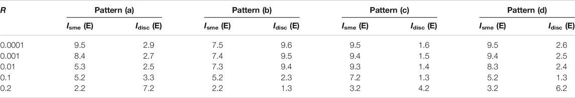
TABLE 1. Condition numbers of element stiffness matrix corresponding to four partition patterns obtained using two integration methods.

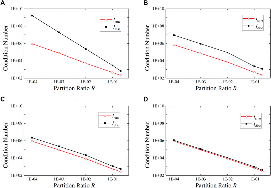
FIGURE 6. Relationship curves of condition number with regard to partition ratio corresponding to four partition patterns (see Figure 5) obtained using two integration methods.

Analysis of Coupling With Interface Contact

For frictional contact problems with interface constraints imposed using the penalty method, the accuracy and stability depend on the penalty parameter k. In this study, a penalty coefficient α was used to define the penalty parameter:

For the case shown in Figure 5A, some interesting phenomena are observed when studying the condition number with different penalty parameters. Here, three rigid-body DOFs must be removed from the enriched DOFs to ensure that the analyzed stiffness matrix is non-singular in the absence of interface constraints.

The influence of interface constraints imposed by the penalty method on element stiffness matrix includes two aspects: 1) The interface constraints restrict relative movements between the two sides of the interface, hence improving the stiffness matrix’s condition. 2) The condition number of the stiffness matrix may increase significantly with a large penalty parameter involved (usually much larger than other parameters in the stiffness matrix).

Table 2; Figure 7 present comparisons of the stiffness matrix condition numbers obtained using smeared and subcell integration with different penalty coefficients and partition ratios. The penalty coefficient α = 0 indicates that no penalty constraint has been imposed. It is observed that as R approached 0, the condition number increased in all cases in a nearly linear manner; however, the condition number corresponding to smeared integration was much smaller than that corresponding to subcell integration, and the increasing slope was much smaller. For subcell integration, the condition number showed almost no change after an interface constraint with a penalty coefficient α = 10 was imposed; the condition number increased significantly with further increase in α, indicating that aspect 2) in the pre-analysis played a dominant role. However, for smeared integration, after an interface constraint with a penalty coefficient α = 10 was imposed, the condition number exhibited a slight decrease; only marginal increase was observed with further increase in α. This indicates that aspect 1) in the pre-analysis played a dominant role. With the coupling of interface contact and internal stiffness, the smeared integration method exhibits a coupling effect that can maintain the stability of the overall condition number, thereby improving the solution stability and the convergence of nonlinear iterations.

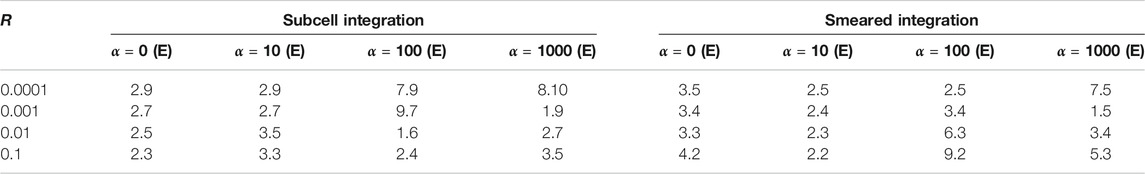
TABLE 2. Condition numbers obtained using two integration methods with different penalty coefficients and partition ratios.

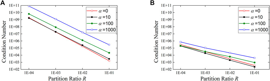
FIGURE 7. Condition numbers obtained using two integration methods with different penalty coefficients and partition ratios. (A) Subcell integration; (B) Smeared integration.

Mixed Integration Scheme for XFEM

When using Newton’s method to solve nonlinear problems, the Jacobian matrix must be updated in each iteration step; the condition number of the Jacobian matrix can significantly affect the stability and convergence of the nonlinear iterations. The iterations can hardly converge with an ill-conditioned Jacobian matrix (Fries and Belytschko, 2010; Belytschko et al., 2014). In practice, an approximate but well-conditioned Jacobian matrix could be better than an accurate but ill-conditioned Jacobian matrix for iteration stability. An approximate Jacobian matrix is commonly employed for problems with an asymmetric Jacobian matrix, such as non-associated elastoplastic constitutive and frictional contact (Chen and Cheng, 2011).

Based on the element analysis of smeared integration presented in the previous section, a mixed integration scheme for XFEM was proposed. A critical partition ratio R* was set, and the stiffness of the element cut by the interface was integrated with respect to the element partition ratio R, as shown in Figure 8. When R was less than R* or greater than 1-R* (the situations in which ill-conditioning occurs), smeared integration was used to improve the stiffness condition; when R was in the middle range, subcell integration was used to obtain a higher integration accuracy. For all residual integrations, subcell integration was used to obtain accurate residuals and ensure accurate results. Based on previous element analyses and the example analyses in next section, the value of R* should be set in the range of 0.05–0.2 to achieve a suitable balance between convergence rate and convergence stability. The partition ratio R, along with the areas or volumes of the subcells and other crack information for a cracked element, are computed in the crack processing procedure once the element reaches the cracking criteria, and are stored for reutilization thereafter. For fixed interface problems mainly discussed in this paper, this information is computed and stored as initial information at the very beginning of the solution.

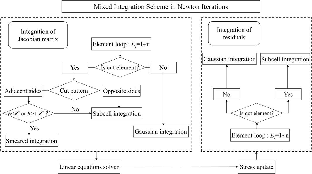
FIGURE 8. Flow chart of mixed integration scheme.

Example Verification

Two typical benchmark examples were used to verify the robustness and practicability of the mixed integration scheme. The global Newton iteration method was used, with $\mathit{r}/{\mathit{r}}_0$ as the convergence indicator for the iteration process, where ${\mathit{r}}_0$ is the initial residual force vector, and r is the residual force vector of the current iteration step, and $\Vert \cdot \Vert$ is the L₂ norm of vectors. The iteration termination conditions were set as

where Niter is the total number of iterations. Condition (Eq. 32-1) indicates that the Newton iteration converges to the given minimum error limit; condition (Eq. 32-2) indicates that after reaching the maximum allowed iteration number, the Newton iteration has not converged to the minimum error limit; condition (Eq. 32-3) indicates that the iteration is divergent.

Frictional Contact Block With Inclined Interface

This example was designed by Dolbow et al. (2001); the model is shown in Figure 9A. It is a square with an inclined interface that passes through the center of the square, separating it into upper and lower parts connected by the interface contact. A displacement load of 0.1 m is applied to the top of the square; the vertical displacement of the bottom is constrained, but is free to move horizontally. The horizontal displacement of the upper right corner of the block is constrained to prevent possible slippage of the entire upper block. The inclination angle of the interface is set at θ = tan⁻¹(0.2). The square has an elastic modulus of E = 1,000 MPa, a Poisson’s ratio of ν = 0.3, and an interface friction coefficient of μ = 0.19. The penalty coefficient is set as α = 10,000.

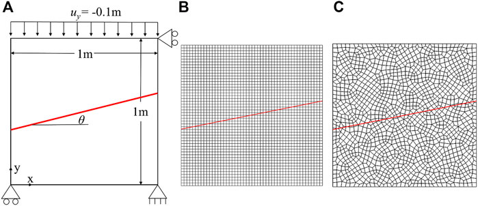
FIGURE 9. Illustration of typical benchmark example. (A) Example model; (B) Regular mesh model; (C) Irregular mesh model.

This example considers a regular mesh and an irregular mesh, as shown in Figures 9B,C, respectively. The regular mesh consists of 40 × 40 square elements. To prevent the interface from passing exactly through the element nodes, the interface is shifted upward by 0.01 m. The irregular mesh consists of 1857 arbitrary quadrilateral elements.

The partition ratio distributions of all cut elements were plotted for both sets of meshes, arranged from small to large, as shown in Figure 10. In both meshes, there were several cut elements with an R value tending to extreme conditions (R < 0.1 and R > 0.9), indicating poor conditions of the Jacobian matrix.

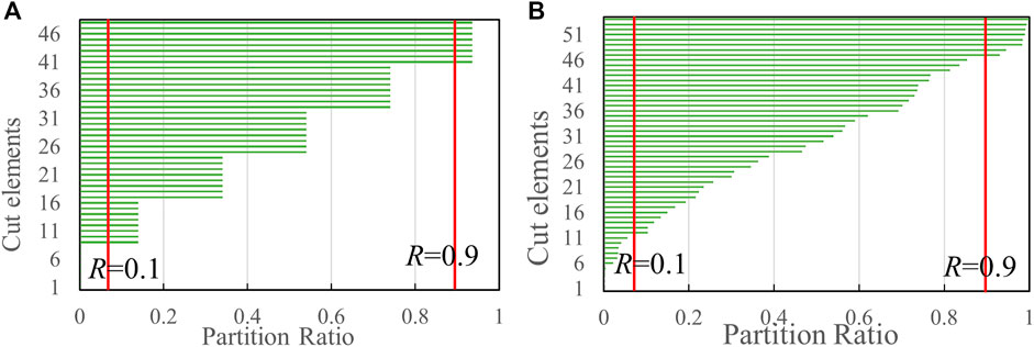
FIGURE 10. Partition ratio distributions of cut elements in two sets of meshes. (A) Regular mesh; (B) Irregular mesh.

The condition numbers of the overall Jacobian matrix for different penalty parameters when using the mixed integration scheme and the total subcell integration scheme are presented in Table 3. For the mixed integration scheme, the critical partition ratio R^* is set as 0.1. The mixed integration scheme significantly reduced the condition number in both meshes; the reductions in the regular and irregular meshes were greater than one order and two orders of magnitude, respectively.

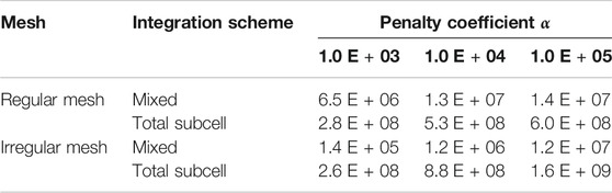
TABLE 3. Condition numbers of Jacobian matrix with different penalty parameters.

A negligible difference was present between the calculation results of the mixed integration scheme and the total subcell integration scheme. A comparison of the calculation results for the regular and irregular meshes also showed a negligible difference. Thus, Figure 11 shows only the displacement contours of the irregular mesh calculated using the mixed integration scheme.

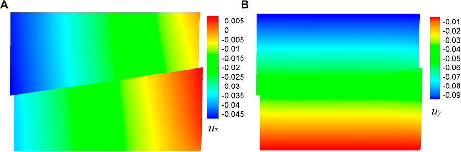
FIGURE 11. Displacement results calculated using mixed scheme with irregular mesh (the displacement is scaled by a factor of 2, Units: m). (A) horizontal displacement; (B) vertical displacement.

The convergence profiles of the two sets of meshes when using the mixed and total subcell integration schemes are shown in Figure 12. For the regular mesh, the total subcell scheme required 14 iteration steps, whereas the mixed scheme required 36 iteration steps to converge to the minimum error limit. This indicates that owing to its approximate Jacobian matrix, the mixed scheme could not reach the optimal Newton convergence rate but can still guarantee convergence. For the irregular mesh, the total subcell scheme could not converge within the Newton iterations, due to the ill-conditioned Jacobian matrix. However, the mixed scheme converged to the minimum error limit after 148 iterations; thus, this scheme can reduce the Jacobian matrix condition number and improve convergence.

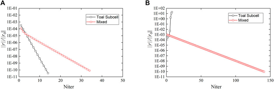
FIGURE 12. Convergence profiles using mixed scheme and total subcell scheme. (A) Regular mesh; (B) Irregular mesh.

3-D Beam Under Uniaxial Tensile Loading

Martin et al. (2015) analyzed a layered 3-D beam under uniaxial tensile loading using XFEM. The beam dimensions and boundary conditions are shown in Figure 13. An interface parallel to the xoy plane divided the beam into upper and lower layers; the tensile stresses applied to the right end of the upper and lower layers were T_up = 300 MPa and T_low = 100 MPa, respectively. The material was an elastoplastic body with linear strain hardening behavior, an elastic modulus of E₀ = 195 GPa, a Poisson’s ratio of ν = 0, a plastic yield strength of ${\sigma }_s$ = 180 MPa, and a strain-hardening modulus (the tangent modulus of the plastic zone) of E_p = 1.95 GPa. This setting resulted in obvious deformation and stress discontinuity in the element cut by the interface. The material above the interface entered the plastic deformation stage, while that below the interface remained elastic. No friction acted on the interface (i.e., the friction coefficient was μ = 0). The normal constraints (non-penetration condition) were imposed using the penalty method, and the penalty coefficient was set as α = 10,000.

FIGURE 13. Setup of 3-D beam problem. (A) xoy plane; (B) yoz plane.

Firstly, a structured hexahedral mesh consisting of 20 × 5 × 3 = 300 elements was used. The splitting of the hexahedral element into tetrahedrons for subcell integration was performed based on the method used by Martin et al. (2015).

The partition ratio of the elements cut by the interface are related with the interface location. For the structured hexahedral mesh, the interface was parallel to one face of the element, and the partition patterns for all elements cut by the interface were the same. The cases with R = 0.5, 0.1, and 0.01, i.e., the interface was located in the middle, upper 90%, and upper 99% of the element, respectively, were analyzed. The critical partition ratio R^* of the mixed integration scheme was set as 0.5. Therefore, the element stiffness of the cut elements in all cases was calculated using the smeared integration method.

Figure 14 shows the calculation results for displacement and stress using the mixed integration scheme, which were consistent with the theoretical solution; the residual errors were less than E-10.

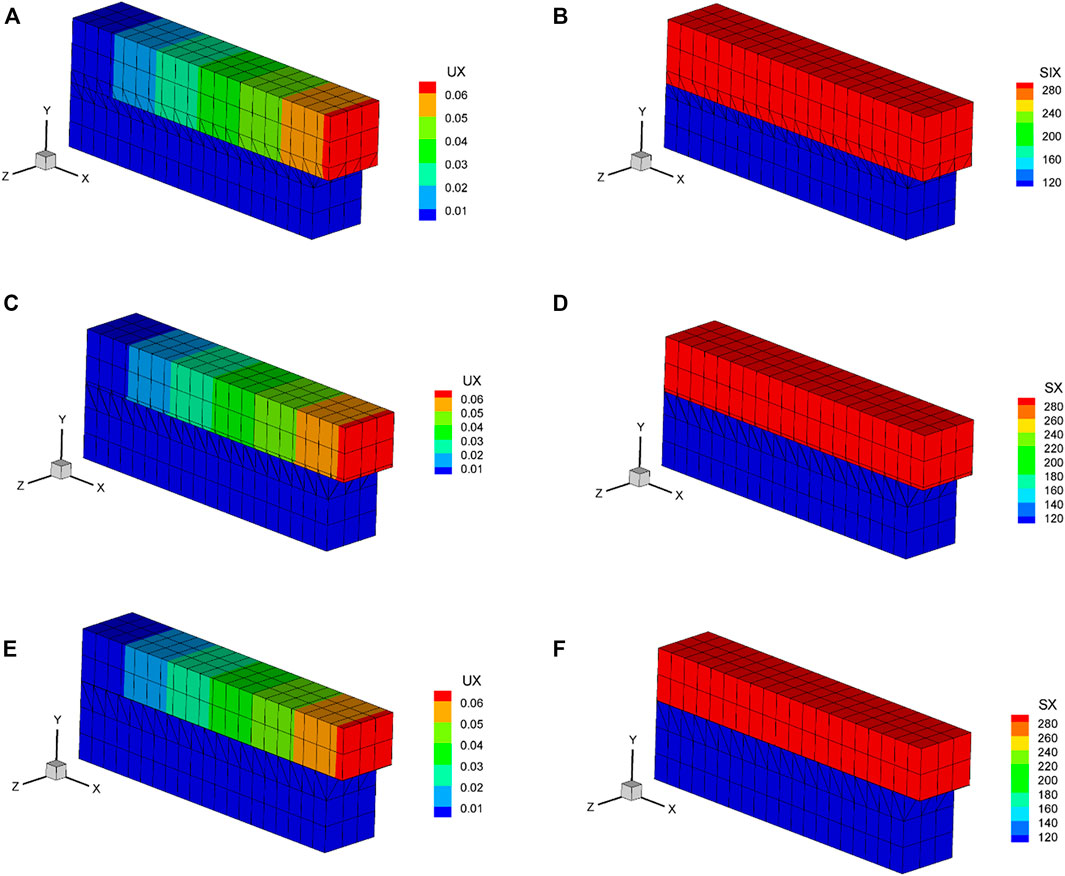
FIGURE 14. Displacement and stress results for structured mesh. (A) x-direction displacement of R = 0.5 (Unit: m); (B) x-direction stress of R = 0.5 (Unit: MPa); (C) x-direction displacement of R = 0.1 (Unit: m); (D) x-direction stress of R = 0.1 (Unit: MPa); (E) x-direction displacement of R = 0.01 (Unit: m); (F) x-direction stress of R = 0.01 (Unit: MPa).

Table 4 presents the condition numbers of the Jacobian matrix with different partition ratios, as obtained using the two integration schemes, when the upper structure entered the plastic stage. At this point, the stiffness difference between the structures above and below the interface was relatively large, leading to relatively large Jacobian matrix condition numbers. The condition numbers increased with a decrease in partition ratio R. For all cases, the mixed integration scheme produced smaller condition numbers than the total subcell scheme.

TABLE 4. Condition numbers of Jacobian matrix with different partition ratios.

The convergence profiles of the two integration schemes with different partition ratios are shown in Figure 15. Owing to accurate integration of the Jacobian matrix, for all three partition ratios, only three iterations were required to converge to a residual error less than E-10 when using the total subcell scheme. However, when using the mixed scheme, 17, 15, and 11 iterations were required to converge to the same error limit for R = 0.5, 0.1, and 0.01, respectively. This result indicates that although the mixed scheme could reduce the Jacobian matrix condition number, it could not achieve the optimal convergence rates, due to approximation of the Jacobian matrix; however, it could guarantee convergence.

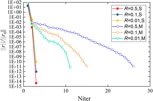
FIGURE 15. Convergence profiles of two integration schemes with different partition ratios (S denotes total subcell scheme and M denotes mixed scheme).

To determine the adaptability of the mixed integration scheme to a more generalized mesh, an unstructured tetrahedral mesh was analyzed. However, it was difficult to avoid the case with the interface very close to some element nodes, which resulted in larger Jacobian matrix condition numbers.

The mesh consisted of 3608 quadratic tetrahedral elements, which yielded a non-constant Jacobian matrix. The vertex nodes were enriched, whereas the edge nodes were not. The interface was described using linearly interpolated level sets defined on the vertex nodes.

A total of 405 elements were cut by the interface; the partition ratio distribution of these elements, arranged from small to large, is shown in Figure 16. For different critical partition ratios R^*, the Jacobian matrix condition numbers under the two integration schemes are presented in Table 5; Figure 17. A smaller R^* indicates a smaller portion of cut elements integrated by the smeared integration method in the mixed scheme. In other words, the smeared integration method plays a less significant role in the mixed scheme; thus, the mixed scheme is more similar to the total subcell scheme. With an increase in R^*, the Jacobian condition number decreases sharply at first, as shown in Table 5; Figure 17. However, after R^* reaches approximately 0.1, the decrease becomes gentle; this indicates that almost all the ill-conditioned elements are included in the smeared integration portion. Thus, the mixed integration scheme can be considered to have reached its limit in terms of the ability to improve the condition of the matrix. Thus, R^* = 0.1 was used in the final calculation.

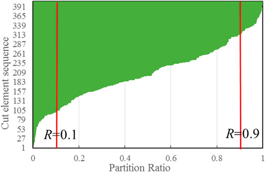
FIGURE 16. Distribution of unstructured mesh partition ratios.

TABLE 5. Condition numbers of Jacobian matrix obtained using two integration schemes with different critical partition ratios.

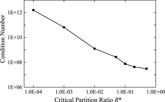
FIGURE 17. Relationship of Jacobian condition numbers using the mixed scheme with critical partition ratios.

The calculation results for stress and displacement using the mixed integration scheme are shown in Figure 18; these results are consistent with the theoretical solution. The mixed scheme converged to the given minimum error limit after 69 iterations, as shown in Figure 19; however, the subcell scheme did not converge within the Newton iterations due to the ill-conditioning. These results prove that the mixed integration scheme exhibits good convergence stability for strongly nonlinear problems with unstructured meshes.

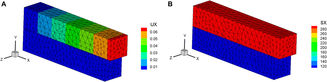
FIGURE 18. Stress and displacement results using mixed integration scheme with unstructured mesh. (A) x-direction displacement (Unit: m); (B) x-direction stress (Unit: MPa).

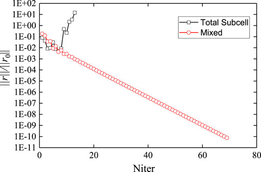
FIGURE 19. Convergence profile of the unstructured mesh for two integration schemes.

Conclusion

This study introduced a smeared integration method that can integrate the weak form of elements with discontinuous enrichment without element splitting. The method also avoids variable mapping in the nonlinear constitutive equations. Compared with conventional methods, this method is simple in form and easy to implement, and achieves excellent performance in terms of improving the condition of system equations. The performance of the method was verified through a series of element analyses. A mixed integration scheme was developed by leveraging the advantages of the smeared integration method and the subcell integration method. To improve the condition and convergence, the smeared integration method was used for the stiffness integration of elements with discontinuous enrichment that may be ill-conditioned; moreover, the subcell method was used for residual integration to ensure the accuracy of the final solution. In the example calculations, the mixed integration scheme significantly improved the system Jacobian condition and provided a good balance between convergence rates and convergence stability, especially with an unstructured mesh.

In general, the proposed integration scheme ensures the convergence of Newton iterations with Jacobian matrix embedded with discontinuous functions, hence promoting the practical application of the extended finite element method in geotechnical and geological disaster assessment and prevention analysis.

Data Availability Statement

The raw data supporting the conclusion of this article will be made available by the authors, without undue reservation.

Author Contributions

PY developed the method and wrote the manuscript. QH performed the engineering application. XW designed the research and participated in writing the manuscript. YY revised and edited the final version. ZZ helped perform the analysis with constructive discussions.

Funding

This work was supported by the National Natural Science Foundation of China (No. U1965206, No. 51979143) and Talents of Guizhou Science and Technology Cooperation Platform ((2018)5630).

Conflict of Interest

Author ZZ was employed by the Power China Guiyang Engineering Co. Ltd.

The remaining authors declare that the research was conducted in the absence of any commercial or financial relationships that could be construed as a potential conflict of interest.

Publisher’s Note

All claims expressed in this article are solely those of the authors and do not necessarily represent those of their affiliated organizations, or those of the publisher, the editors and the reviewers. Any product that may be evaluated in this article, or claim that may be made by its manufacturer, is not guaranteed or endorsed by the publisher.

Supplementary Material

The Supplementary Material for this article can be found online at: https://www.frontiersin.org/articles/10.3389/feart.2021.829203/full#supplementary-material

Footnotes

¹The red lines represent the discontinuous interfaces, and the arrows point toward the side where H(x) > 0. Along the arrow direction, the discontinuous interfaces gradually approach the element node, and the value of R gradually decreases to zero

²I_sme denotes smeared integration; I_disc denotes subcell integration

References

Abdelaziz, Y., and Hamouine, A. (2008). A Survey of the Extended Finite Element. Comput. Structures 86 (11), 1141–1151. doi:10.1016/j.compstruc.2007.11.001
Abedian, A., and Düster, A. (2019). Equivalent Legendre Polynomials: Numerical Integration of Discontinuous Functions in the Finite Element Methods. Comput. Methods Appl. Mech. Eng. 343, 690–720. doi:10.1016/j.cma.2018.08.002
Agathos, K., Bordas, S. P. A., and Chatzi, E. (2019). Improving the Conditioning of XFEM/GFEM for Fracture Mechanics Problems through Enrichment Quasi-Orthogonalization. Comput. Methods Appl. Mech. Eng. 346, 1051–1073. doi:10.1016/j.cma.2018.08.007
Béchet, E., Minnebo, H., Moës, N., and Burgardt, B. (2005). Improved Implementation and Robustness Study of the X-FEM for Stress Analysis Around Cracks. Int. J. Numer. Meth. Engng 64 (8), 1033–1056. doi:10.1002/nme.1386
Belytschko, T., and Black, T. (1999). Elastic Crack Growth in Finite Elements with Minimal Remeshing. Int. J. Numer. Meth. Engng. 45 (5), 601–620. doi:10.1002/(sici)1097-0207(19990620)45:5<601:aid-nme598>3.0.co;2-s
Belytschko, T., Gracie, R., and Ventura, G. (2009). A Review of Extended/generalized Finite Element Methods for Material Modeling. Model. Simul. Mater. Sci. Eng. 17 (4), 043001. doi:10.1088/0965-0393/17/4/043001
Belytschko, T., Liu, W. K., Moran, B., and Elkhodary, K. (2014). Nonlinear Finite Elements for Continua and Structures. Hoboken, NJ, USA: John Wiley & Sons. doi:10.13140/RG.2.1.2800.0089
Belytschko, T., Moës, N., Usui, S., and Parimi, C. (2001). Arbitrary Discontinuities in Finite Elements. Int. J. Numer. Meth. Engng. 50 (4), 993–1013. doi:10.1002/1097-0207(20010210)50:4<993:aid-nme164>3.0.co;2-m
Bordas, S., Nguyen, P. V., Dunant, C., Guidoum, A., and Nguyen-Dang, H. (2007). An Extended Finite Element Library. Int. J. Numer. Meth. Engng 71, 703–732. doi:10.1002/nme.1966
Chen, X., and Cheng, Y. G. (2011). On Accelerated Symmetric Stiffness Techniques for Non‐associated Plasticity with Application to Soil Problems. Eng. Computations 28 (8), 1044–1063. doi:10.1108/02644401111179027
Chin, E. B., Lasserre, J. B., and Sukumar, N. (2017). Modeling Crack Discontinuities without Element‐partitioning in the Extended Finite Element Method. Int. J. Numer. Meth. Engng 110 (11), 1021–1048. doi:10.1002/nme.570410.1002/nme.5436
Choi, Y. J., Hulsen, M. A., and Meijer, H. E. H. (2012). Simulation of the Flow of a Viscoelastic Fluid Around a Stationary cylinder Using an Extended Finite Element Method. Comput. Fluids 57, 183–194. doi:10.1016/j.compfluid.2011.12.020
Cruz, F., Roehl, D., and Vargas, E. d. A. (2019). An XFEM Implementation in Abaqus to Model Intersections between Fractures in Porous Rocks. Comput. Geotechnics 112, 135–146. doi:10.1016/j.compgeo.2019.04.014
Daux, C., Moës, N., Dolbow, J., Sukumar, N., and Belytschko, T. (2000). Arbitrary Branched and Intersecting Cracks with the Extended Finite Element Method. Int. J. Numer. Meth. Engng. 48, 1741–1760. doi:10.1002/1097-0207(20000830)48:12<1741:aid-nme956>3.0.co;2-l
Dolbow, J., Moës, N., and Belytschko, T. (2001). An Extended Finite Element Method for Modeling Crack Growth with Frictional Contact. Comput. Method Appl. M 190 (51), 6825–6846. doi:10.1016/S0045-7825(01)00260-2
Fries, T.-P., and Belytschko, T. (2010). The Extended/generalized Finite Element Method: An Overview of the Method and its Applications. Int. J. Numer. Meth. Engng. 84 (3), 253–304. doi:10.1002/nme.2914
Gracie, R., and Craig, J. R. (2010). Modelling Well Leakage in Multilayer Aquifer Systems Using the Extended Finite Element Method. Finite Elem. Anal. Des. 46, 504–513. doi:10.1016/j.finel.2010.01.006
Joulaian, M., Hubrich, S., and Düster, A. (2016). Numerical Integration of Discontinuities on Arbitrary Domains Based on Moment Fitting. Comput. Mech. 57 (6), 979–999. doi:10.1007/s00466-016-1273-3
Kumar, S., and Bhardwaj, G. (2018). A New Enrichment Scheme in XFEM to Model Crack Growth Behavior in Ductile Materials. Theor. Appl. Fracture Mech. 96, 296–307. doi:10.1016/j.tafmec.2018.05.008
Li, H., Li, J., and Yuan, H. (2018). A Review of the Extended Finite Element Method on Macrocrack and Microcrack Growth Simulations. Theor. Appl. Fracture Mech. 97, 236–249. doi:10.1016/j.tafmec.2018.08.008
Martin, A., Esnault, J.-B., and Massin, P. (2015). About the Use of Standard Integration Schemes for X-FEM in Solid Mechanics Plasticity. Comput. Methods Appl. Mech. Eng. 283, 551–572. doi:10.1016/j.cma.2014.09.028
Matthew, G. P., and Caglar, O. (2016). Three-Dimensional Modeling of Short Fiber-Reinforced Composites with Extended Finite-Element Method. J. Eng. Mech. 142, 04016087. doi:10.1061/(ASCE)EM.1943-7889.0001149
Moës, N., Dolbow, J., and Belytschko, T. (1999). A Finite Element Method for Crack Growth without Remeshing. Int. J. Numer. Meth Eng. 46 (1), 131–150. doi:10.1002/(SICI)1097-0207(19990910)46:1<131:AID-NME726>3.0.CO
Natarajan, S., Bordas, S., and Roy Mahapatra, D. (2009). Numerical Integration over Arbitrary Polygonal Domains Based on Schwarz-Christoffel Conformal Mapping. Int. J. Numer. Meth. Engng. 80 (1), 103–134. doi:10.1002/nme.2589
Natarajan, S., Mahapatra, D. R., and Bordas, S. P. A. (2010). Integrating strong and Weak Discontinuities without Integration Subcells and Example Applications in an XFEM/GFEM Framework. Int. J. Numer. Meth. Engng. 83 (3), 269–294. doi:10.1002/nme.2798
Reusken, A. (2008). Analysis of an Extended Pressure Finite Element Space for Two-phase Incompressible Flows. Comput. Vis. Sci. 11, 293–305. doi:10.1007/s00791-008-0099-8
Salimzadeh, S., and Khalili, N. (2015). A Three-phase XFEM Model for Hydraulic Fracturing with Cohesive Crack Propagation. Comput. Geotechnics 69, 82–92. doi:10.1016/j.compgeo.2015.05.001
Sauerland, H., and Fries, T.-P. (2013). The Stable XFEM for Two-phase Flows. Comput. Fluids 87, 41–49. doi:10.1016/j.compfluid.2012.10.017
Song, J.-H., Areias, P. M. A., and Belytschko, T. (2006). A Method for Dynamic Crack and Shear Band Propagation with Phantom Nodes. Int. J. Numer. Meth. Engng 67 (6), 868–893. doi:10.1002/nme.1652
Sukumar, N., Dolbow, J. E., and Moës, N. (2015). Extended Finite Element Method in Computational Fracture Mechanics: a Retrospective Examination. Int. J. Fract 196 (1-2), 189–206. doi:10.1007/s10704-015-0064-8
Ventura, G., and Benvenuti, E. (2015). Equivalent Polynomials for Quadrature in Heaviside Function Enriched Elements. Int. J. Numer. Meth. Engng 102 (3-4), 688–710. doi:10.1002/nme.4679
Ventura, G. (2006). On the Elimination of Quadrature Subcells for Discontinuous Functions in the eXtended Finite-Element Method. Int. J. Numer. Meth. Engng 66 (5), 761–795. doi:10.1002/nme.1570
Ventura, G., and Tesei, C. (2016). Stabilized X-FEM for Heaviside and Nonlinear Enrichments. New York: Springer International Publishing, 209–228. doi:10.1007/978-3-319-41246-7_10
Wang, X.-N., Yu, P., Zhang, X.-T., Yu, J.-L., Hao, Q.-S., Li, Q.-M., et al. (2021). Simulation of Three-Dimensional Tension-Induced Cracks Based on Cracking Potential Function-Incorporated Extended Finite Element Method. J. Cent. South. Univ. 28 (1), 235–246. doi:10.1007/s11771-021-4599-8
Wang, X., Yu, P., Yu, J., Yu, Y., and Lv, H. (2018). Simulated Crack and Slip Plane Propagation in Soil Slopes with Embedded Discontinuities Using XFEM. Int. J. Geomech. 18 (12), 04018170. doi:10.1061/(ASCE)GM.1943-5622.0001290
Keywords: mixed integration, XFEM, smeared integration, convergence, nonlinear iteration, ill-conditioning
Citation: Yu P, Hao Q, Wang X, Yu Y and Zhan Z (2022) Mixed Integration Scheme for Embedded Discontinuous Interfaces by Extended Finite Element Method. Front. Earth Sci. 9:829203. doi: 10.3389/feart.2021.829203
Received: 05 December 2021; Accepted: 22 December 2021;
Published: 21 January 2022.
Edited by:
Xiaodong Fu, Institute of Rock and Soil Mechanics (CAS), ChinaReviewed by:
Zhu Jun-Gao, Hohai University, ChinaXi Chen, Beijing Jiaotong University, China
Degao Zou, Dalian University of Technology, China
Copyright © 2022 Yu, Hao, Wang, Yu and Zhan. This is an open-access article distributed under the terms of the Creative Commons Attribution License (CC BY). The use, distribution or reproduction in other forums is permitted, provided the original author(s) and the copyright owner(s) are credited and that the original publication in this journal is cited, in accordance with accepted academic practice. No use, distribution or reproduction is permitted which does not comply with these terms.
*Correspondence: Xiangnan Wang, 13684060651@163.com