Real-Time Dispatching Performance Improvement of Multiple Multi-Energy Supply Microgrids Using Neural Network Based Approximate Dynamic Programming
 Bei Li
 Robin Roche
- 1College of Chemistry and Environmental Engineering, Shenzhen University, Shenzhen, China
- 2FEMTO-ST, FCLAB, UTBM, CNRS, University Bourgogne Franche-Comté, Belfort, France
In the multi-energy supply microgrid, different types of energy can be scheduled from a “global” view, which can improve the energy utilization efficiency. In addition, hydrogen storage system performs as the long-term storage is considered, which can promote more renewable energy installed in the local consumer side. However, when there are large numbers of grid-connected multi-energy microgrids, the scheduling of these multiple microgrids in real-time is a problem. Because different types of devices, three types of energy, and three types of utility grid networks are considered, which make the dispatching problem difficult. In this paper, a two-stage coordinated algorithm is adopted to operate the microgrids: day-ahead scheduling and real-time dispatching. In order to reduce the time taken to solve the scheduling problem, and improve the scheduling performance, approximate dynamic programming (ADP) is used in real-time operation. Different types of value function approximations (VFA), i.e., linear function, nonlinear function, and neural network are compared to study about the influence of the VFA on the decision results. Offline and online processes are developed to study the impact of the historical data on the regression of VFA. The results show that the neural network based ADP one-step decision algorithm has almost the same performance as the Global optimization algorithm, and the highest performance among all others Local optimization algorithms. The total operation cost relative error is less than 3%, while the running time is only 31% of the Global algorithm. In the neural network based ADP, the key technology is continuously updating the training dataset online, and adopting an appropriate neural network structure, which can at last improve the scheduling performance.
1 Introduction
Hydrogen storage based multi-energy supply microgrids are expected to play an important role in future smart cities (Mancarella, 2014; Li et al., 2017b). In a multi-energy supply microgrid, several load demands are covered, such as electricity/heat/gas. At the same time, a hydrogen storage system can be used to alleviate the intermittence of renewable energy. For the hydrogen storage system, when the renewable energy is redundant, surplus energy is converted to hydrogen (
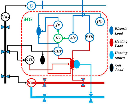
FIGURE 1. Multi-energy supply microgrid.
On the other hand, multi-energy supply microgrids can also interconnect with different utility grids (electricity/heat/gas) (Li et al., 2018b). The structure of utility grids is shown in Figure 2. The left network represents the electricity supply system, the middle network is the gas supply system, and the right network is the heat supply system. With this integrated utility grid networks, local loads can better resist to the natural disasters (Wang et al., 2016). For example, if the electric utility grid is destroyed under natural disasters, the gas utility grid system can supply gas to a fuel cell to produce electricity. Then the local loads can still operate.
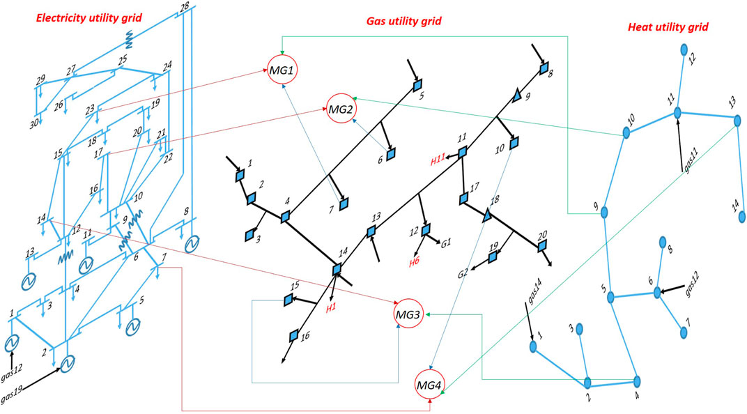
FIGURE 2. The structure of the multiple energy supply network.
However, operating these multi-energy supply grid-connected microgrids in real-time is still a problem. Because different types of devices, three types of energy, and three types of utility grid networks are considered, which make the dispatching problem difficult.
In fact, the microgrid operation problem is often formulated as a model predictive control (MPC) problem, because MPC is widely accepted in varieties of industrial scenarios, and its effective ability to deal with optimization problems subject to large numbers of constraints (Shang and You, 2019). In fact, several methods can be adopted to solve the MPC problem.
The first category is heuristic algorithms, such as GA (Li et al., 2017a), PSO (Mohammadi-Ivatloo et al., 2013), etc. which are largely employed to solve the microgrid operation problem. This is due to their flexibility and the possibility to face complex constraints. However, heuristic algorithms do not guarantee obtaining an optimal results, because the solution is updated based on stochastic searching.
The second category is mixed integer programming (MIP). This is due to the availability of efficient commercial software, such as CPLEX and Gurobi (Gurobi, 2018). For example, in (Li and Xu, 2019), authors study the operation of a multi-energy microgrid under diverse uncertainties. The problem is represented as a two-stage operation problem. And at last is converted to a mixed-integer linear programming (MILP) problem. In (Li et al., 2021), authors study the optimal deployment of energy storage in a residential multi-energy microgrid. Based on the linearisation method, the model is converted to a MILP problem. However, in the MIP problem, the number of optimization windows is an important parameter. When the number of optimization windows is large, the solving time is long, because the variables needed to decide are large. When the number of optimization windows is small, the variables needed to decide are small, the solving time is then short, but the results are far away from the global optimal points, because more future impacts are not considered. So, the trade-off between window numbers and solving time should be considered.
The third category is dynamic programming (Xie et al., 2017), which transfers the long time horizon MPC problem into a series of smaller problems that can be easily solved. But dynamic programming suffers from the “curse-of-dimensionality” (Shi et al., 2017), which makes it difficult to use in real-time operation of large systems.
Then, a method is required which can efficiently and quickly solve the optimization problem in real-time, where the results are not far away from the global optimal points.
Approximate dynamic programming (ADP) method can resolve this problem. ADP method is a one-step decision model, and the future influence is considered as a value function approximation (VFA) in the current decision. This means that if we can find a good VFA, we can then quantify the future influence well, which leads to a reasonable decision at the current time. Since ADP is just one-step, the problem-solving time is faster than the multiple windows MPC method.
Therefore, in this paper, we adopt the ADP method to control the optimal operation of grid-connected microgrids. We focus on the performance of the ADP method and compare different factors, such as regression methods, offline/online process, and so on.
1.1 Scheduling Problem Based on Approximate Dynamic Programming
For the ADP method, the main thing is the value function approximation. In general, there are three methods to describe the value function approximation (Salas and Powell, 2013; Li and Jayaweera, 2015): lookup table, parametric approximation and nonparametric approximation. For example, in (Das and Ni, 2018), authors research about the battery storage systems operation in islanded microgrid considering battery lifetime characteristics, and the approximate value function is formulated based on lookup table idea. In (Li and Jayaweera, 2015), the authors use Q-learning method to define the approximate value function. In (Keerthisinghe et al., 2018), the piecewise linear function is used to build the approximate value function. In (Zeng et al., 2018), deep recurrent neural network learning is adopted to describe the approximate value function. The reference papers showed that ADP has better performance and lower computational burden.
Using the ADP method to optimal control the operation of microgrids has also attracted lots of attention.
1.1.1 Lookup Table and Parametric Approximate Value Function
In (Keerthisinghe et al., 2018), the authors present an ADP-based smart home energy management system. Lookup tables and piecewise linear functions are used to define approximate value function, the results show that the ADP-based algorithm reduces the daily electricity cost without an increase in the computational burden. In Salas and Powell (2013), authors present an ADP method to control the operation of the energy storage systems to achieve an economical goal. Piecewise linear function is adopted to define approximate value function. In (Jiang et al., 2014), the authors compare different ADP methods for energy storage control problem, including approximate policy iteration and approximate value iteration. In (Anderson et al., 2011), the authors apply ADP to the smart grid dispatching problem. The long-time horizon scheduling problem is transferred into a series of smaller problems, which is easier to be solved.
Authors in (Strelec and Berka, 2013), present the ADP method to solve multi-energy supply microgrid economic dispatching problems, lookup table and regression methods are used to approximate the cost function. In (Shuai et al., 2018b), the authors propose the lookup table based ADP algorithm for the real-time energy management of the microgrid under uncertainties. The dispatching problem is formulated as a long-time horizon mixed integer nonlinear programming model and is then decomposed into several single period nonlinear programming sub-problems based on ADP method. Similarly, in (Shuai et al., 2018a), a piecewise linear function based ADP algorithm is adopted to solve the stochastic microgrid economic dispatching problem. Authors in (Darivianakis et al., 2017), transfer the MPC optimal problem into VFA based multi-stage optimization problem, a piecewise linear function is adopted to approximate the value function. Authors in (Bhattacharya et al., 2018) present a two-stage dual dynamic programming method to manage energy storage in a microgrid, a piecewise linear function is also adopted to approximate cost-to-go functions.
1.1.2 Nonparametric Approximate Value Function
In (Ji et al., 2018), authors research about real-time economical operation of a grid-connected microgrid using the ADP method. Multilayer perceptron feedforward neural network is adopted to approximate value function. In (Zeng et al., 2018), the authors study the economical operation of a microgrid in real-time. ADP and deep recurrent neural network (RNN) learning are adopted to solve the problem. Deep RNN architecture is used to estimate the value function. Furthermore, authors in (Liu et al., 2015) present an approximate dynamic programming algorithms for solving undiscounted optimal control problems. Two multilayer feedforward neural networks are used to approximate both the control policy and the value function. In order to enhance the resource utilization rate and reduce the computation cost, authors in (Wang et al., 2019) present an event-based iterative adaptive critic algorithm, in which three neural networks are constructed but possessing different roles. That is: the model network employed for prediction, the critic network built for evaluation, and the action network used for control. In order to tackle dynamic uncertainties, authors in (Wang, 2019) study robust policy learning control for nonlinear plants. Neural network based actor-critic structure is designed to implement the robust control.
Authors in (Zhu et al., 2019) research the optimal management of multiple batteries over a long time horizon in order to prolong battery lifetime. Approximate dynamic programming is adopted to solve the problem, and fuzzy systems are used to approximate value functions. Compared to neural networks, the fuzzy approximation only requires to compute target values.
Based on the above papers, the ADP method is effective to solve the dispatching problem, and the ADP method can be divided into the following steps as: 1) build the dispatching optimization model; 2) transfer the multi-step decision problem into a series of one-step decision problems; 3) find the relationship between the states and future costs, using lookup table/regression/neural network methods to describe the relationship, namely, build the approximate value function; 4) integrate the approximate value function into the one-step decision model; 5) solve the approximate value function based one-step decision problem.
1.2 Electricity/Heat/Gas Utility Grids Operation
The above section reviews the related work about scheduling algorithms for microgrid. In addition, when microgrid interconnects with the electricity/heat/gas utility grids, the operation of the electricity/heat/gas utility grids should also be considered.
For the coupled multi-energy networks operation, centralized optimization algorithm is often used to solve the optimal power flow. For example, authors in (Qin et al., 2020) study the operation of integrated energy systems consisting of electricity and natural gas utility networks, a multi-objective optimization method is used to solve the coordinated operation of the coupling network. In (Sun et al., 2020), authors study the day-ahead scheduling of gas-electric integrated energy system considering the bi-directional energy flow. The goal is to minimize the operation cost, and a second-order cone programming method is utilized to solve the problem. In (Fang et al., 2018), authors study the operation of the integrated gas and electrical power system considering the different response times of the gas and power systems. The problem is transformed into a single-stage linear programming. In (Chen et al., 2017), authors study the optimal operation of electricity-gas integrated energy system. The goal is to minimize the operation costs for both electrical and natural gas systems while satisfying steady-state operational constraints.
To model the electricity/heat/gas utility grid networks. The steady-state operational equations are often built as the constraints, and added to the previous optimization problem. For example, in (Liu et al., 2020), authors present a sequential reliability assessment method considering multi-energy flow and thermal inertia. Hydraulic circulation and heat exchange equations are used to model the thermal network. Conventional power flow equations are adopted to describe distribution network model. In (Martínez Ceseña et al., 2020), the electricity network model is represented as conventional power flow equations, as well as thermal and voltage limits. The gas network is represented as steady-state equations. The conventional steady-state equations and a thermal module are utilized to model the heat network. In (Yang et al., 2020), authors present a planning strategy for a district energy sector considering the coupling of power, gas, and heat systems. An optimal multi-energy flow model is developed, and the objective is to minimize operational costs. Distflow equations are used to describe the power distribution system, steady gas flow equations are adopted to model the gas distribution system, steady-state model is deployed to describe the distribution heat system. In (Martínez Ceseña and Mancarella, 2019), authors present a robust optimization framework for smart districts with multi-energy devices and electricity/heat/gas energy networks. The electricity network is modelled with typical power flow equations. The heat network is described based on nodal balance and cumulative head losses equations. The gas network is represented based on nodal balance, pressure drops, and head losses equations.
Based on the above reviews, optimization method is often used to calculate the power flow of the electricity/heat/gas energy networks. The electricity network is modelled based on typical power flow equations. The heat network is modelled based on nodal balance and heat losses equations. The gas network is represented based on nodal balance, pressure drops equations.
1.3 Contributions
The above review shows that the operation problem of multi-energy supply microgrid and the operation problem of coupled electricity/heat/gas energy networks have drawn a lot of attention. However, using the ADP algorithm to solve the dispatching problem of the hydrogen-based multi-energy supply microgrids considering electricity/heat/gas energy networks has not drawn a lot of attention. The complexity of the whole model increases the difficulty of the control, especially the large numbers of constraints. Motivated by the aforementioned references, we present an ADP-based computationally efficient algorithm for the real-time operation of multi-energy supply grid-connected microgrids. A similar study is our previous work (Li et al., 2018a), in which only MPC algorithm is used, no other algorithms are compared.
Compared to previous works, the contribution of this paper can be concluded as follows:
• First, we build an ADP-based one-step decision model for the optimal operation of multi-energy supply grid-connected microgrids. In the one-step decision model, we consider large numbers of logical and physical constraints, and formulate the problem as a mixed-integer programming model;
• Second, in the ADP model, we research about different factors. Linear, nonlinear, and neural network regression are compared to research about the influence of the approximate value function on the decision results. Offline and online processes are developed to research about the impact of the historical data on the regression approximate value function;
• Last, we compare the performance of the sliding window MPC, the one-step decision ADP and the global optimization algorithms from different perspectives, including the running time, the real-time operation cost, total operation cost, and the exchanged energy with the utility grid networks. The results show that the neural network based ADP method has the best performance, with the less than 3% total operation cost relative error, and has a running time of only 31% of Global algorithm.
The remainder of this paper is organized as follows. Section 2 describes the microgrid scheduling problem. Section 3 describes the electricity/heat/gas utility grids model. Section 6 presents the simulation results. Finally, Section 7 concludes the paper.
In fact, to operate the electricity/heat/gas integrated microgrids system, three aspects should be considered: 1) scheduling of the grid-connected microgrid; 2) utility grids operation; 3) the operation of the whole system.
2 Microgrid Scheduling Problem Formulation
To schedule the grid-connected microgrids, the coordinated strategy is often adopted, namely, day-ahead scheduling and real-time dispatching. In day-ahead scheduling, the expected exchange energy with utility grids are calculated, based on the exchanged energy, we can decide the role of the microgrids, namely, microgrids operate as a generator or as a load. In real-time dispatching, the ADP-based one-step decision problem is solved. It takes the future operation cost into consideration and makes the current dispatching more reasonable, and at the same time reduces the solving time.
We introduce the problem from three aspects: 1) day-ahead scheduling; 2) real-time dispatching based on MPC; 3) real-time dispatching based on ADP.
2.1 Microgrid Day-Ahead Scheduling
In order to make the problem more readable, we use the simple model to describe the problem, and the detailed model is attached in Supplementary Material. The scheduling problem can be described as follows:
where
By solving the above mixed integer programming problem, we can obtain the scheduling results. However, due to the uncertainty of the load demand and the output of renewable energy, some parameters in constraints are not deterministic parameters. The above problem is then transferred to the following problem:
where
The common method to solve the above uncertainty problem is stochastic optimization. The above problem can be transferred as follows:
In the above stochastic problem, we use a scenario-based method to transfer the uncertainty parameters
Assume that the variables that exchanged energy with utility grids are
2.2 Microgrid Real-Time Dispatching Based on MPC
Based on the day-ahead scheduling results, we can then implement real-time dispatching. Due to the real-time short-term prediction uncertainty, the real-time exchanged energy with the utility grid may not equal to the day-ahead scheduling results. In order to reduce this error, it is necessary for the real-time exchanged energy to follow the day-ahead scheduling results as close as possible. The sliding window model predictive control method is then adopted to deploy the real-time dispatching, the detailed model is attached in Supplementary Material. The real-time dispatching problem can be described as follows:
where
In the real-time sliding window dispatching, in the first time step t, the MPC problem is solved, then only the current time decisions (current time is t) are deployed, and the future decisions (future times are
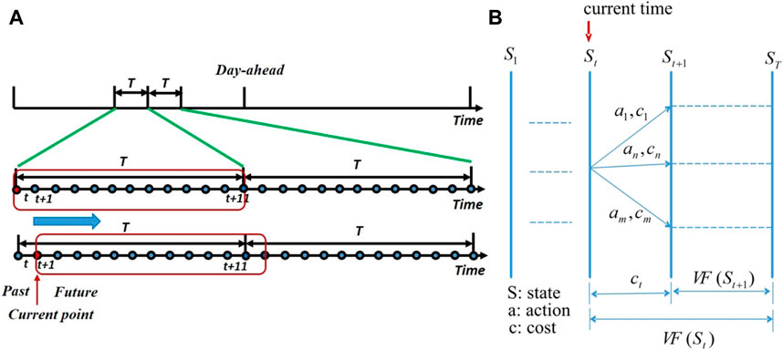
FIGURE 3. (A) Sliding window model predictive control. (B) The state transition process.
2.3 Microgrid Real-Time Dispatching Based on ADP Method
In the above section, the sliding window MPC method is adopted to deploy real-time dispatching. However, the solving time of the MPC method is long, because we need to solve the multiple windows optimization problem. In this section, the one-step decision model is developed to solve the real-time dispatching problem. With the one-step decision model, the solving time can be reduced. On the other hand, the ADP idea is also adopted, namely, integrating the future impacts into the current decision model, to make the current decision results more reasonable and effective.
In fact, the above MPC problem can be transferred into a series of smaller problems based on dynamic programming idea, which can be represented as follows:
We use
Then the above problem can be represented as:
Because the future cost
where
By solving the above one-step decision model (namely, the decision variables are only at the current time), one can obtain the optimal dispatching results. However, it can be seen that the main thing in the above one-step decision model is the approximate value function
2.3.1 Approximate Value Function
The approximate value function
where
With the approximate value function
Firstly, we need to obtain the historical dataset of
Secondly, we need to analyze the dataset to find the relationship between
In the linear regression method, we use function
At last, we developed offline and online processes to deploy the ADP method. In the offline process, at each time t, there are four steps: 1) update the dataset
Algorithm 1 Offline simulation process.
1: initialize dataset
2: for
3: update the dataset
4: calculate the approximate value function
5: linear method:
6: nonlinear method:
7: neural network method:
8: solve the problem Eq. 9;
9:
10: save the operation results;
11: t = t+1;
12: end for
In the online process, there is not enough initial dataset, so the dataset is obtained and updated based on the online operation. At each time t, the process is run
Algorithm 2 Online simulation process
1: initialize
2: for
3: initialize the dataset
4: for
5: update the dataset
6: calculate the approximate value function
7: linear method:
8: solve the problem Eq. 9;
9:
10: save the operation results;
11: i = i + 1;
12: end for.
13: t = t + 1;
14: end for
2.3.2 ADP State Transition Process
The state transition process can be seen in Figure 3B. It can be seen that future approximate operation cost
3 Utility Grids Operation Problem
For the integrated utility grids model, an IEEE30 + gas20 + heat14 hybrid network is adopted. The structure of each utility grid network is presented in Supplementary Material.
3.1 Electricity Utility Grid Operation
For the electricity utility grid operation, it is a classical optimal power flow (OPF) problem. The OPF problem can be seen as follows:
where the
Power balance constraints can be shown as the following:
where
where
3.2 Heating Utility Grid Operation
For the heating utility grid, it is a heating power flow problem. During the heating transportation, heat transportation loss should be considered. The heating transportation loss can be described as follows (Pirouti, 2013; Shabanpour-Haghighi and Seifi, 2015).
where
The temperature drop through the heating flow system can be described as:
where l is the pipe length, U is the heat transition coefficient (W/mK), and
Based on (Eqs. 14Eqs. 15), it can be seen that the heating loss during the transportation is a nonlinear equation. In order to reduce the complexity, in this paper, we choose a linear model to describe the heating transportation loss. We assume that the heating loss is a linear function of the transportation distance, which can be shown as the following:
where
Then, the heating power flow of the heating utility grid can be presented. For each heating pipeline, two state variables (binary variables, 0 or 1):
An example is presented here to explain the logical illustrated in Eq. 18. In Eq. 18, there are three nodes
3.3 Gas Utility Grid Operation
For the gas utility grid, it is a gas power flow problem. The gas flow can be described as follows (De Wolf and Smeers, 2000):
where
During the gas transportation, the pressure will drop, which is modeled as in Eq. 21.
Based on Eqs. 20Eqs. 21, we can obtain
Then, the gas pressure drop can be described as:
Assume that the loss
In (Martinez-Mares and Fuerte-Esquivel, 2012), it shows that the pressure drop
where
Then the gas power flow in the gas utility grid can be presented. For each pipeline, two state variables (binary variables, 0 or 1)
Here we also use an example to explain the gas flow, which is shown in Eq. 25. There are three nodes
The gas flow in a gas pipeline is restricted by the pressure of the beginning and end nodes. This constraint can be described as:
where
4 The Sequential Operation of the Whole System
Four microgrids are interconnected with the hybrid IEEE30 + gas20 + heat14 network. It is actually difficult to schedule this complex system. In this paper, we present a sequential strategy as follows: 1) first, four microgrids run their scheduling algorithms based on MPC or ADP method [section (2)], and obtain the exchanged energy with electricity/heat/gas utility grids; 2) second, the utility grids receive the exchanged energy, and run their power flow problem [Section (3)].
5 System Setup
In this paper, an IEEE-30 + gas-20 + heat-14 hybrid system is adopted as the utility grids. Four multi-energy microgrids are connected with the utility grids. The structure is presented in Figure 2. Microgrid MG1 is connected at electrical node e23, gas node g7, heat node h9. Microgrid MG2 is connected at electrical node e17, gas node g6, heat node h10. Microgrid MG3 is connected at electrical node e14, gas node g15, heat node h4. Microgrid MG4 is connected at electrical node e7, gas node g10, heat node h13. The configutation of this hybrid system is summarized in Eq. 28. The model is implemented in MATLAB and solved with YALMIP (Löfberg, 2012) and Gurobi.
A typical day is chosen. Based on the forecasted load demands and PV output, microgrids firstly run their day-ahead scheduling algorithm, and the exchanged energy results with the utility grids are obtained and then transferred to the real-time dispatching algorithm. Secondly, the real-time rolling horizon dispatching algorithm is solved based on the new forecasting data and the day-ahead exchange results.
The load demands (peak load) of each microgrid and microgrid operation parameters are presented in Supplementary Material.
6 Simulation Results
Based on the above strategy, the simulation running is deployed. The simulation results are presented from four aspects: 1) scheduling results; 2) operation cost analysis; 3) exchanged energy analysis; 4) utility grids power flow.
6.1 Scheduling Results
Different cases are presented to research about the performance of each algorithm. Cases
1.
2.
3.
4.
5.
6.
7.
8.
9.
10.
11.
12.
13.
14.
The simulation results of the real-time SOC of MG4 can be seen in Figure 4. Here SOC means the percentage of hydrogen in tanks. It can be seen that with different algorithms, the real-time dispatching results are significantly different. This is because in different algorithms, the future operation value functions are different, leading to different scheduling results.
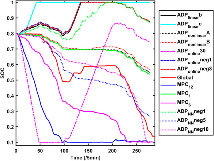
FIGURE 4. Real-time SOC of MG4 with different optimization algorithms.
We compare these different algorithms in the following:
where
where
where
where
where
where
In Figure 4, we set the case
We compare different
The linear regression of value function is shown in Figure 5B.
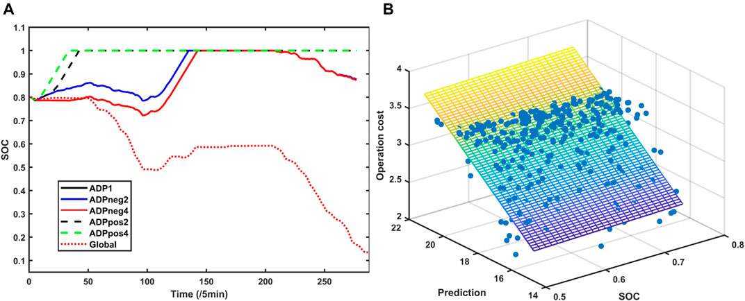
FIGURE 5. (A) Real-time SOC of MG4 with different linear value functions. (B) Linear regression of value function.
In fact, case
Then, we adopt the nonlinear function to regress the dataset. And we compare different
The nonlinear regression of value function is shown in Figure 6B.
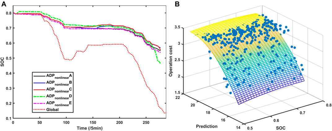
FIGURE 6. (A) Real-time SOC of MG4 with different nonlinear value functions. (B) Nonlinear regression of value function.
It can be seen that based on the nonlinear approximate value function, the scheduling results have similar tendency to the global results. And with different coefficients
After that we adopt the neural network to regress the dataset. And we compare different
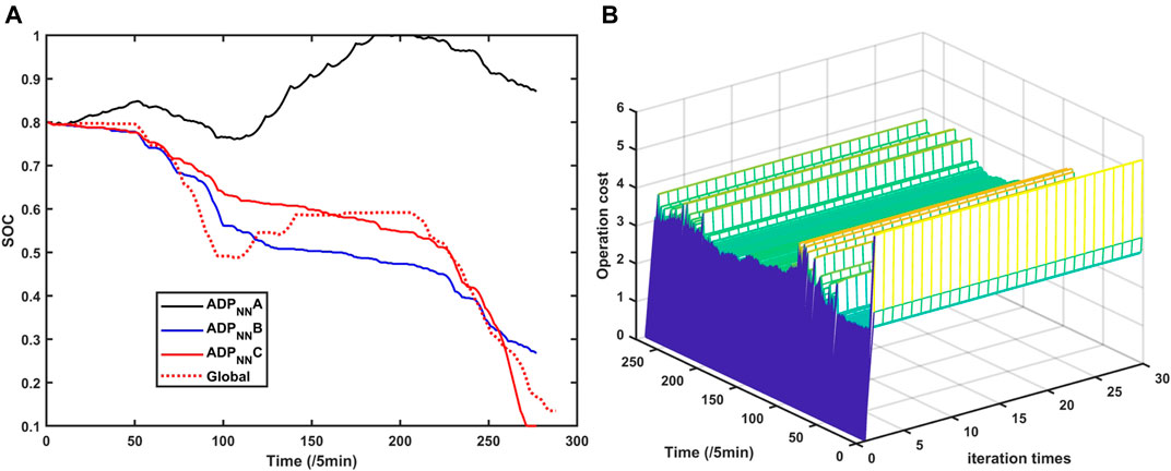
FIGURE 7. (A) Neural network regression of the value function. (B) Operation cost of MG4 based on the online ADP method.
It can be seen that based on the neural network approximate value function, if we choose the approximate coefficients, the scheduling results are very close to the global optimization results, which means that the neural network can regress the value function well.
After that we develop an online simulation process, namely, at each time, the one-step decision model is iteratively simulated 30 times. The simulated operation cost of MG4 is shown in Figure 7B.
At each time, the one-step optimization model is solved for 30 times, and in each iteration, the parameters of the approximate value function is updated. Based on Figure 7B, it can be seen that at each time step, after 30 times iteration, the operation costs keep constantly, which means that the iteration process is convergence.
6.2 Operation Cost Analysis
In this section, we analyze the operation cost of MGs based on different algorithms. Operation costs are the results of the problem Eq. 29 and problem Eq. 34. We use a 2-norm error to describe the difference between real-time operation cost of different algorithms and global optimization. The 2-norm error can be represented as:
where
Table 1 shows the 2-norm error of real-time operation cost of MG4 with different algorithms. It can be seen that
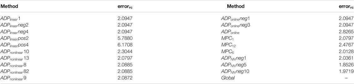
TABLE 1. Real-time operation cost 2-norm error of MG4 with different algorithms.
We then compare the total operation cost (total time horizon) in Table 2 and Figure 8. It can be seen that case
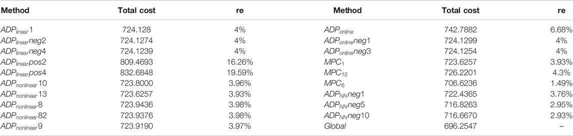
TABLE 2. Total operation costs.
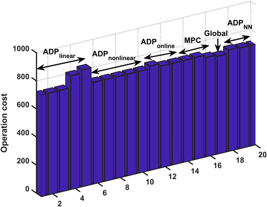
FIGURE 8. Total operation cost based on different algorithms.
Then, we need to choose an index to evaluate different algorithms. Here, we use relative error
where
We can then calculate the relative error with different algorithms, which is shown in Table 2. It can be seen that in case
In the online case
For the MPC cases, the optimization window number is important, it can be seen that when the optimization window number is 6, the relative error is less than 1.5%; and the sliding window is 12, the relative error is about 4.3%. For the
At last, from the post-event analysis view (total operation cost), it can be seen that algorithm
In conclusion, different algorithms have advantages and disadvantages, we choose four indexes to compare these algorithms: running time, one-step simulation time τ, results, and complexity, which can be seen in Table 3.
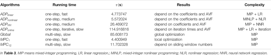
TABLE 3. Comparison of different algorithms.
6.3 Exchanged Energy With Utility Grids
The exchanged electricity/heat/gas with utility grids are shown in Figures 9, 10, 11A. In order to make these figures readable, we calculate the 2-norm error of the exchanged energy under different algorithms (case “Global” is set as the basic case), which is shown in Table 4.
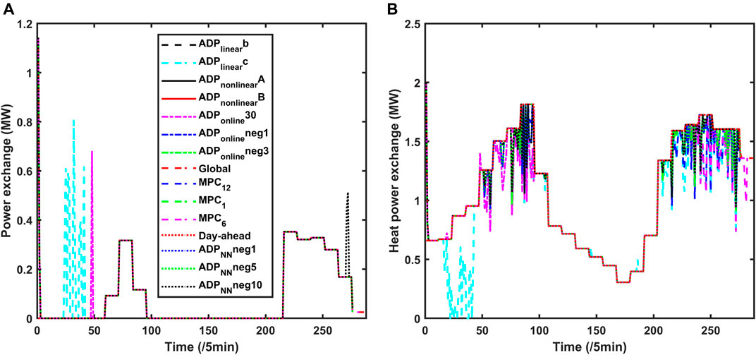
FIGURE 9. (A) Electricity power exchange with utility grid under different algorithms. (B) Heat power exchange with utility grid under different algorithms.
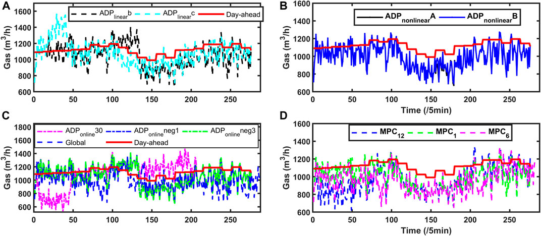
FIGURE 10. (A) Gas exchange with utility grid with
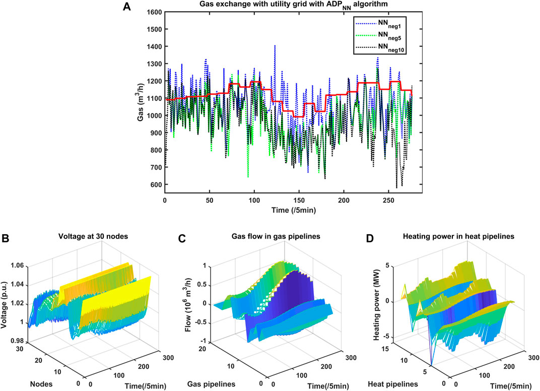
FIGURE 11. (A) Gas exchange with utility grid with
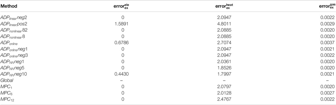
TABLE 4. 2-norm error of the exchanged energy with different algorithms.
For the exchanged electricity, cases
For the exchanged heat, it can be seen that cases
For the exchange gas, cases
At last, overall consideration of
6.4 Utility Grids Power Flow
Based on the above exchanged energy, the electricity/heat/gas utility grids then run their power flow algorithm. The voltage of the IEEE-30 node electricity network with
7 Conclusion
In this paper, the real-time operation of grid-connected microgrid based on ADP algorithm was studied, a hybrid multi-energy supply microgrid model was adopted. We focused on studying the performance of different scheduling algorithms. Day-ahead stochastic scheduling and real-time dispatching coordinated strategy was adopted.
For the day-ahead scheduling, the scenario-based stochastic optimization was used. For the real-time dispatching, ADP and MPC algorithms were adopted, different parameters and coefficients were compared to study the performance of each algorithm.
Based on the simulation results, some conclusions were presented:
1) ADP and MPC algorithm had the ability to implement the real-time operation. Linear function based AVF ADP algorithm, one optimization window number MPC algorithm had a fast running time. Nonlinear function based AVF ADP algorithm had an average running time. Online process ADP method, global optimization and multiple window numbers MPC algorithm had a slow running time.
2) In the ADP method, AVF was the important parameter to influence the dispatching results. In fact, neural network based AVF ADP algorithm had the smallest real-time operation cost 2-norm error, less than 3% total operation cost relative error, and the smallest exchanged energy 2-norm error, which means that neural network based AVF ADP had the best performance. In addition, the running time of neural network based AVF ADP was only 31% of the Global algorithm.
3) In the online process, because there was not enough initial dataset, the regression AVF could not better describe the future operation cost, which leaded to an average performance. In addition, at each time step, the real-time optimization problem was iteratively solved for several times, which also increased the running time. However, the online process provided a method to make the decision when there was not enough initial dataset.
In conclusion, we presented a neural network based ADP real-time dispatching algorithm, which had almost the same performance with Global optimization, while only 31% running time of the Global algorithm. It can be directly utilized in industry scenarios and improve the dispatching performance compared to MPC algorithm.
Data Availability Statement
The original contributions presented in the study are included in the article/Supplementary Material, further inquiries can be directed to the corresponding author.
Author Contributions
BL: Conceptualization, Methodology, Software, Writing- Original draft preparation, Reviewing and Editing. RR: Visualization, Investigation, Validation, Reviewing and Editing.
Funding
This work has been supported by the “Guangdong Basic and Applied Basic Research Foundation” (2019A1515110641), the “Fundamental Research Funds for the Shenzhen university” (000002110235), the EIPHI Graduate School (contract ANR-17-EURE-0002), and the Region Bourgogne-Franche-Comté.
Conflict of Interest
The authors declare that the research was conducted in the absence of any commercial or financial relationships that could be construed as a potential conflict of interest.
Supplementary Material
The Supplementary Material for this article can be found online at: https://www.frontiersin.org/articles/10.3389/felec.2021.637736/full#supplementary-material.
References
Anderson, R. N., Boulanger, A., Powell, W. B., and Scott, W. (2011). Adaptive stochastic control for the smart grid. Proc. IEEE 99, 1098–1115. doi:10.1109/JPROC.2011.2109671
Bhattacharya, A., Kharoufeh, J. P., and Zeng, B. (2018). Managing energy storage in microgrids: a multistage stochastic programming approach. IEEE Trans. Smart Grid 9, 483–496. doi:10.1109/TSG.2016.2618621
Chen, S., Wei, Z., Sun, G., Cheung, K. W., and Wang, D. (2017). Identifying optimal energy flow solvability in electricity-gas integrated energy systems. IEEE Trans. Sustain. Energy 8, 846–854. doi:10.1109/TSTE.2016.2623631
Darivianakis, G., Eichler, A., Smith, R. S., and Lygeros, J. (2017). A data-driven stochastic optimization approach to the seasonal storage energy management. IEEE Control Syst. Lett. 1, 394–399. doi:10.1109/LCSYS.2017.2714426
Das, A., and Ni, Z. (2018). A computationally efficient optimization approach for battery systems in islanded microgrid. IEEE Trans. Smart Grid 9, 6489–6499. doi:10.1109/TSG.2017.2713947
De Wolf, D., and Smeers, Y. (2000). The gas transmission problem solved by an extension of the simplex algorithm. Manag. Sci. 46, 1454–1465. doi:10.1287/mnsc.46.11.1454.12087
Fang, J., Zeng, Q., Ai, X., Chen, Z., and Wen, J. (2018). Dynamic optimal energy flow in the integrated natural gas and electrical power systems. IEEE Trans. Sustain. Energy 9, 188–198. doi:10.1109/TSTE.2017.2717600
Ji, Y., Wang, J., Fang, X., and Zhang, H. (2018). “Online optimal operation of microgrid using approximate dynamic programming under uncertain environment,” in 2018 37th Chinese control conference (CCC), Wuhan, China, July 25–27, 2018 (New York, NY: IEEE), 2235–2241. doi:10.23919/ChiCC.2018.8483355
Jiang, D. R., Pham, T. V., Powell, W. B., Salas, D. F., and Scott, W. R. (2014). “A comparison of approximate dynamic programming techniques on benchmark energy storage problems: does anything work?” in 2014 IEEE Symposium on adaptive dynamic programming and reinforcement learning (ADPRL), Orlando, FL, December 9–12, 2014 (New York, NY: IEEE), 1–8. doi:10.1109/ADPRL.2014.7010626
Keerthisinghe, C., Verbic, G., and Chapman, A. C. (2018). A fast technique for smart home management: adp with temporal difference learning. IEEE Trans. Smart Grid 9, 3291–3303. doi:10.1109/TSG.2016.2629470
Löfberg, J. (2012). Automatic robust convex programming. Optim. Methods Softw. 27, 115–129. doi:10.1080/10556788.2010.517532
Li, B., Roche, R., and Miraoui, A. (2017a). Microgrid sizing with combined evolutionary algorithm and milp unit commitment. Appl. Energy 188, 547–562. doi:10.1016/j.apenergy.2016.12.038
Li, B., Roche, R., Paire, D., and Miraoui, A. (2017b). Sizing of a stand-alone microgrid considering electric power, cooling/heating, hydrogen loads and hydrogen storage degradation, Appl. Energy 205, 1244–1259. doi:10.1016/j.apenergy.2017.08.142
Li, B., Roche, R., Paire, D., and Miraoui, A. (2018a). Coordinated scheduling of a gas/electricity/heat supply network considering temporal-spatial electric vehicle demands. Electr. Power Syst. Res. 163, 382–395. doi:10.1016/j.epsr.2018.07.014
Li, B., Roche, R., Paire, D., and Miraoui, A. (2018b). Optimal sizing of distributed generation in gas/electricity/heat supply networks. Energy 151, 675–688. doi:10.1016/j.energy.2018.03.080
Li, D., and Jayaweera, S. K. (2015). Machine-learning aided optimal customer decisions for an interactive smart grid. IEEE Syst. J. 9, 1529–1540. doi:10.1109/JSYST.2014.2334637
Li, Z., and Xu, Y. (2019). Temporally-coordinated optimal operation of a multi-energy microgrid under diverse uncertainties. Appl. Energy 240, 719–729. doi:10.1016/j.apenergy.2019.02.085
Li, Z., Xu, Y., Feng, X., and Wu, Q. (2021). Optimal stochastic deployment of heterogeneous energy storage in a residential multienergy microgrid with demand-side management. IEEE Trans. Industr. Inform. 17, 991–1004. doi:10.1109/TII.2020.2971227
Liu, D., Li, H., and Wang, D. (2015). Error bounds of adaptive dynamic programming algorithms for solving undiscounted optimal control problems. IEEE Trans. Neural Netw. Learn. Syst. 26, 1323–1334. doi:10.1109/TNNLS.2015.2402203
Liu, W., Ma, T., and Yang, Y. (2020). Reliability assessment of integrated energy system based on coupling energy flow and thermal inertia. CSEE J. Power Energy Syst. 1–11. doi:10.17775/CSEEJPES.2019.03030
Mancarella, P. (2014). Mes (multi-energy systems): an overview of concepts and evaluation models. Energy 65, 1–17. doi:10.1016/j.energy.2013.10.041
Martínez Ceseña, E. A., Loukarakis, E., Good, N., and Mancarella, P. (2020). Integrated electricity-heat-gas systems: techno-economic modeling, optimization, and application to multienergy districts. Proc. IEEE 108, 1392–1410. doi:10.1109/JPROC.2020.2989382
Martínez Ceseña, E. A., and Mancarella, P. (2019). Energy systems integration in smart districts: robust optimisation of multi-energy flows in integrated electricity, heat and gas networks. IEEE Trans. Smart Grid 10, 1122–1131. doi:10.1109/TSG.2018.2828146
Martinez-Mares, A., and Fuerte-Esquivel, C. R. (2012). A unified gas and power flow analysis in natural gas and electricity coupled networks. IEEE Trans. Power Syst. 27, 2156–2166. doi:10.1109/tpwrs.2012.2191984
Mohammadi-Ivatloo, B., Moradi-Dalvand, M., and Rabiee, A. (2013). Combined heat and power economic dispatch problem solution using particle swarm optimization with time varying acceleration coefficients. Electr. Power Syst. Res. 95, 9–18. doi:10.1016/j.epsr.2012.08.005
Pirouti, M. (2013). Modelling and analysis of a district heating network. PhD thesis. Cardiff (United Kingdom): Cardiff University.
Qin, Y., Wu, L., Zheng, J., Li, M., Jing, Z., Wu, Q. H., et al. (2020). Optimal operation of integrated energy systems subject to coupled demand constraints of electricity and natural gas. CSEE J. Power Energy Syst. 6, 444–457. doi:10.17775/CSEEJPES.2018.00640
Salas, D. F., and Powell, W. B. (2013). Benchmarking a scalable approximate dynamic programming algorithm for stochastic control of multidimensional energy storage problems. Informs J. Comput. 30, 106–123. doi:10.1287/ijoc.2017.0768
Shabanpour-Haghighi, A., and Seifi, A. R. (2015). Simultaneous integrated optimal energy flow of electricity, gas, and heat. Energy Convers. Manag. 101, 579–591. doi:10.1016/j.enconman.2015.06.002
Shang, C., and You, F. (2019). A data-driven robust optimization approach to scenario-based stochastic model predictive control. J. Process Contr. 75, 24–39. doi:10.1016/j.jprocont.2018.12.013
Shi, W., Li, N., Chu, C.-C., and Gadh, R. (2017). Real-time energy management in microgrids. IEEE Trans. Smart Grid 8, 228–238. doi:10.1109/tsg.2015.2462294
Shuai, H., Fang, J., Ai, X., Tang, Y., Wen, J., and He, H. (2018a). Stochastic optimization of economic dispatch for microgrid based on approximate dynamic programming. IEEE Trans. Smart Grid 10, 2440–2452. doi:10.1109/TSG.2018.2798039
Shuai, H., Fang, J., Ai, X., Wen, J., and He, H. (2018b). Optimal real-time operation strategy for microgrid: an ADP based stochastic nonlinear optimization approach. IEEE Trans. Sustain. Energy 10, 931–942. doi:10.1109/TSTE.2018.2855039
Strelec, M., and Berka, J. (2013). “Microgrid energy management based on approximate dynamic programming,” in IEEE PES ISGT Europe 2013, Lyngby, Denmark, October 6–13, 2013 (New York, NY: IEEE), 1–5. doi:10.1109/ISGTEurope.2013.6695439
Sun, Y., Zhang, B., Ge, L., Sidorov, D., Wang, J., and Xu, Z. (2020). Day-ahead optimization schedule for gas-electric integrated energy system based on second-order cone programming. CSEE J. Power Energy Syst. 6, 142–151. doi:10.17775/CSEEJPES.2019.00860
Wang, D. (2019). Robust policy learning control of nonlinear plants with case studies for a power system application. IEEE Trans. Industr. Inform. 16, 1733. doi:10.1109/TII.2019.2925632
Wang, D., Ha, M., and Qiao, J. (2019). Self-learning optimal regulation for discrete-time nonlinear systems under event-driven formulation. IEEE Trans. Automat. Contr. 65, 1272. doi:10.1109/TAC.2019.2926167
Wang, Y., Chen, C., Wang, J., and Baldick, R. (2016). Research on resilience of power systems under natural disasters – a review. IEEE Trans. Power Syst. 31, 1604–1613. doi:10.1109/TPWRS.2015.2429656
Xie, S., He, H., and Peng, J. (2017). An energy management strategy based on stochastic model predictive control for plug-in hybrid electric buses. Appl. Energy 196, 279–288. doi:10.1016/j.apenergy.2016.12.112
Yang, W., Liu, W., Chung, C. Y., and Wen, F. (2020). Coordinated planning strategy for integrated energy systems in a district energy sector. IEEE Trans. Sustain. Energy 11, 1807–1819. doi:10.1109/TSTE.2019.2941418
Zeng, P., Li, H., He, H., and Li, S. (2018). Dynamic energy management of a microgrid using approximate dynamic programming and deep recurrent neural network learning. IEEE Trans. Smart Grid 10, 4435. doi:10.1109/TSG.2018.2859821
Keywords: real-time scheduling, gas/electricity/heat, approximate dynamic programming, neural network, microgrid
Citation: Li B and Roche R (2021) Real-Time Dispatching Performance Improvement of Multiple Multi-Energy Supply Microgrids Using Neural Network Based Approximate Dynamic Programming. Front. Electron. 2:637736. doi: 10.3389/felec.2021.637736
Received: 04 December 2020; Accepted: 26 January 2021;
Published: 12 April 2021.
Edited by:
Rui Zhang, University of New South Wales, AustraliaReviewed by:
Yuhua Du, Temple University, United StatesZhengmao Li, Nanyang Technological University, Singapore
Copyright © 2021 Li and Roche. This is an open-access article distributed under the terms of the Creative Commons Attribution License (CC BY). The use, distribution or reproduction in other forums is permitted, provided the original author(s) and the copyright owner(s) are credited and that the original publication in this journal is cited, in accordance with accepted academic practice. No use, distribution or reproduction is permitted which does not comply with these terms.
*Correspondence: Bei Li, bei.li@szu.edu.cn