Communicating Hydrological Hazard-Prone Areas in Italy With Geospatial Probability Maps

Introduction

Changes in the frequency of severe weather events determine the occurrence of damaging hydrological events (Diodato et al., 2019; Petrucci et al., 2019), which in turn affect many natural and human systems (Corella et al., 2016; Sofia et al., 2017). Modeling rainfall intensity can help to quantifying the effect of these extreme phenomena that involve complex landscape and ecosystem scenarios within multiple event feedback forms (e.g., Thomas, 2001; Mulligan and Wainwright, 2013; Harris et al., 2018).

Water is certainly a resource for the Earth's ecosystems, but intense rainfall and overland flows can also be land disturbing forces. Extreme hydro-meteorological events such as rainstorms produce high-impact land processes, which increases with their intensity (Toy et al., 2002; Wei et al., 2009). However, diverse parts of the terrestrial ecosystems respond in different ways to unequal forcing agents, often non-linear and universal, with threshold-type characteristics (Thomas, 2001; Arnell, 2011; Knight and Harrison, 2013; Seddon et al., 2016). Simultaneous mapping of these thresholds, and the processes for developing them, is a challenge in geographical information sciences (Srivastava, 2013; Li et al., 2016). The scale and the relative uncertainty integration of these thresholds, for which storms drive overland flows, including the soil erosion by water, are important because they affect the spatial pattern of damaging hydrological events, and ultimately improve our mechanistic understanding of ecological responses to climate extremes (Kayler et al., 2015). An example of rainfall threshold-driven process is the initiation of landslides (Guzzetti et al., 2007). Concepts such as thresholds of change and magnitude are all important since landscapes may be able to resist or absorb impulses of change as a form of sensitivity or, inversely, stability (Huggett, 1988; Meyer et al., 2018). The application of this concept to the way how geomorphological systems respond to climatic variability and change is nowadays a relevant topic (Allison and Thomas, 1993; Phillips, 2006). In geomorphology, the first use of sensitivity has been in the form of a ratio between resisting to and disturbing forces, inherently changing, but natural systems generally have a high capacity to absorb such changes (Brunsden, 2001). Research indicates that distinct ways in which sensitivity analysis is applied have different implications, because whereas the ratio of resisting to disturbing forces is dimensionless, landforms within a landscape may react differently to environmental events, possibly owing to varied proximity to a particular threshold, which introduces an element of probability related to the likelihood of change (Downs and Gregory, 1993). Thus, in this work the erosivity density (MJ ha⁻¹ h⁻¹ mm⁻¹), that is, the ratio of rainfall erosivity to precipitation, is introduced to measure the erosivity per rainfall unit. The critical value of erosivity density ≥3 MJ ha⁻¹ h⁻¹ has been introduced in storm geomorphology by Dabney et al. (2011). This hydrological threshold could help identify erosion- and overland flow-prone areas (Kinnell, 2010; Panagos et al., 2016). The advantages of using erosivity density over directly calculated rainfall erosivity are (after Renard et al., 2011): (a) higher susceptibility to classifying hydrological hazards; (b) higher stability, achieved with a shorter period of records; and (c) easier interpolation over large territories owing to its altitude-independency up to 3,000 m a.s.l. (Foster et al., 2003).

Uncertainty in erosivity density thresholds poses challenges for the spatial analysis since the worst storms may fall in areas between recording weather stations (e.g., Willmott and Legates, 1991). The summer season in Mediterranean lands is characterized by aggressive storms developing the risk for damaging hydrology and catastrophic events (Pereira et al., 2010; Diodato et al., 2011; Diakakis et al., 2018; Salvati et al., 2018). Local interactions between environmental context and climate variability are provided as comprehensive explanation for landscape changes and impact evaluation (Bintliff, 2002). The diverse geomorphology characterizing the Mediterranean region has important consequences for the atmospheric and sea circulations, with an uneven distribution of weather types (Lionello et al., 2006) and a broad spectrum of hydro-geomorphological hazard potentials across Italy (Diodato et al., 2019).

Throughout the Mediterranean basin (including Italy), rainfall is typically concentrated between autumn and spring (Trigo et al., 2006) but extreme hydrological and geomorphological events occur mainly in periods of imbalance of precipitation input, from May to October. Though only a few studies have explicitly investigated how precipitation affects the damaging hydrological events in this vulnerable period of the year (Cevasco et al., 2015), in recent years, a considerable progress has been made in developing rainfall erosivity databases from regional (Borrelli et al., 2016) to continental scale (Panagos et al., 2015) and even to global (Panagos et al., 2017) scale. However, the development of regional-scale spatial models of the storm hazard remains a challenge that scientists face for hydrological, agricultural, and environmental planning. The spatial uncertainty associated with the danger of extreme rainfall across a range of scales is an open issue, which is added to uncertainties associated with downscaling methods and lack of high temporal resolution data in many regions.

The present paper has the main objective of demonstrating to which extent the threshold associated with erosivity densities depends on hydrological damaging events prediction of. A coupled GIS and geostatistics model is the tool, applied here, to continuously map the spatial uncertainty of erosivity density thresholds and predict prone areas to damaging hydrological events in Italy. The achieved results are funded on climatic data and on a probabilistic approach. Other parameters, affecting the intensity and the frequency of damage in risk-prone areas as population density, infrastructures, plants density, and low-intensity rainy periods have not considered as out of the scopus of the present work.

Materials and Methods

Study Area and Data Collection

The Mediterranean has the highest amounts of precipitation during the period October to March, while mean summer precipitation is less predictable owing to high rainfall variance in this season (Xoplaki et al., 2004). Moreover, the period between end of summer and beginning of autumn results in considerable percentage of bare and tilled soils (compared to green cover) across the Mediterranean, including Italy. This agro-environmental condition accelerates the hazard of severe erosion and overland flow (Pereira et al., 2010). In this period, the sparser the plant cover, the more vulnerable the topsoil is to both dislodgement and removal by raindrop impact and surface runoff. As with spatial variability, the temporal variation in precipitation and vegetation response are non-linearly related, highlighting the existence of threshold behaviors, which are heterogeneous in dynamic, changing landscapes (Snyder and Tartowski, 2006).

The Italian territory is characterized by heterogeneous geographic systems, with sea surface waters around the Italian peninsula, where vast mountain chains, coexist with valleys and plains. The most southern part of Italy is an active storm area, and its orography is an important agent in modifying the track of cyclones and their synoptic evolution across Europe (Homar and Stensrud, 2004). Such heterogeneity modifies mesoscale components of the circulation and generates precipitation patterns fluctuating greatly in space or time (Luterbacher et al., 2012). Convective rainfall events, in particular, cause extreme, and erosive storms, which are geographically localized in Italy. Such large spatial and temporal variability can be difficult to capture accurately with rain gauge networks or remote sensing observations (Curić and Janc, 2011). Advective rainfall, in contrast, is characterized by weak rainfall intensity over large areas.

In this study, data on rainfall erosivity and precipitation were derived from the Rainfall Erosivity Database on the European Scale (REDES) (Panagos et al., 2015). 219 uniformly distributed meteorological stations were selected in order to cover the different biogeographical and climate zones of Italy (Figures 1A,B) with an average density of about one station per 1,000 km²: The stations‘ elevation ranges from 0 to 2,541 m a.s.l. with a distribution reflecting the altitudinal gradients of the country. The frequency of acquisition of precipitation data is hourly over a period larger than 10 years (2002–2011). The grid-based map of rainfall erosivity density was created interpolating the data resources represented by 219 stations.

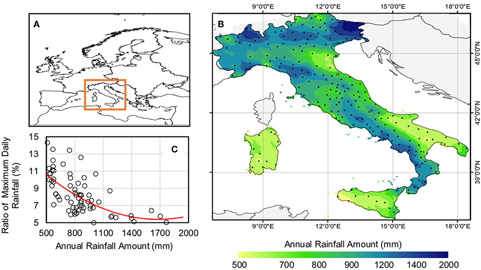
Figure 1. (A) Overview map of the study area. (B) The spatial pattern of mean annual rainfall amount overlaid with stations location, and (C) Ratio of maximum-recorded daily rainfall vs. mean annual precipitation for Italy during the period 2002–2011.

Erosivity Density Model

In an erosive climate, the magnitude, intensity, and frequency of a given precipitation has an impact in damaging hydrological processes as it changes both landform and the equilibrium of environmental systems. The assumption, in order to model the erosivity density (ED), is that the environmental system adapts to changes of the natural hydrological regime. In fact a fluctuation in such regime, especially when thresholds for an acceptable level of hydrological disturbance are exceeded, may have damaging consequences to the environment.

The ED algorithm, which predicts damaging hydrological hazards, is based on the ratio between storm erosivity and precipitation (Dabney et al., 2011; Renard et al., 2011):

where n is the number of recorded years; m_j is the number of erosive events during a given month j; k is the index of a k^th single event; v_r is the rainfall volume (mm) during the r^th period of a storm, which splits into m parts; I₃₀ is the maximum 30-min rainfall intensity (mm h⁻¹); i_r is the rainfall intensity during the time interval (mm h⁻¹); P_j is the rainfall amount (mm) during a given month j.

Therefore, the numerator in Equation (1) represents the mean monthly storm erosivity (MJ mm ha⁻¹ h⁻¹), while the denominator the relative average precipitation amount (mm) multiplied by a factor f .

The variables involved can be subjected to large time fluctuations and set threshold in the natural hydro-geomorphological regime, in such a case the coefficient f is a useful parameter to explain the degree of local ecosystem flexibility, whose estimate is required for the geomorphological risk assessment within given features (Diodato, 2005). In fact, natural land-based ecosystems can be quite flexible and capable of absorbing the stresses provoked by disturbance in a vast array of processes (Mendoza et al., 2002), including the damages associated with weather extremes (De Luís et al., 2001), so that f >1. Contrarily, highly disturbed or degraded landscapes (e.g., intensive cropland, chaotic urbanization, post-fire vegetation dynamics, sparse vegetation), are commonly less flexible, so that f < 1.

According to Dabney et al. (2011), when ED>3 MJ ha⁻¹ h⁻¹, storm erosivity accounts for a large percentage of the rainfall amount in an intense event, highlighting an increasing erosive hazard (above the critical value for damaging hydrological events).

Probability kriging and Fit of the Regional Model

Geostatistical techniques consider that distant data values are less related to each other than near spatial data values (after Tobler, 1970). The commonly used ordinary kriging (OK), in particular, computes an unsampled value (z), knowing its coordinates (x, y), and neighbor values. OK makes optimal, unbiased estimates of regionalized variables at unsampled points from values of the same variables at surrounding stations, using structural analysis and the initial set of measured data (Journel and Huijbregts, 1978; Journel, 1983). Kriging-type approaches are probabilistic in nature because the uncertainty associated with a local estimate can be calculated. OK of a set of indicator-transformed values provides a resultant value between 0 and 1 for each point estimate. This is an estimate of the proportion of the values in the neighborhood, which are greater than the indicator or threshold value. Probability kriging (PK) was proposed by Sullivan (1984) to overcome some issues raised with indicator kriging (IK) which is a non-parametric approach to estimate data uncertainty and is used to predict conditional probability (e.g., probability of the occurrence of an event above/below a threshold) for categorical data of unsampled location. Probability kriging is a non-linear method, which uses the information from all the available indicator variables by using the order relation of observed variables. It represents an attempt to obtain estimates less sensitive than the ones obtained with IK to the choice and number of cut-off values (thresholds). In addition, compared to IK, the estimates of PK fully reflect local variability (Hohn, 1999). PK can be used to classify areas under damaging hydrological hazard prone areas. A straightforward approach is to classify as hazardous all locations where the probability of exceeding a critical threshold value, z_k, is greater than a critical value of erosivity density (ED = 3 MJ ha⁻¹ h⁻¹). Kriging methods rely on the notion of autocorrelation. Correlation is usually thought of as the tendency for two or more variables to be related. For example, in climate sciences, weather stations close to each other have similar climatic values. When weather stations become distant, then climatic values are different. In the same way, in geo-statistics, locations distant from measured climatic data may have high prediction uncertainty. The rate at which the correlation decays can be expressed as a function of distance and at some distance to weather stations, the pixel values have no correlation with the prediction location. Based on this assumption, a search neighborhood function (here below cdf) is generally specified (see result section) that limits the number and the configuration of the measured data points that will be used in the prediction. The mechanism controlling the radius of the neighborhood function shape is mainly driven from the range, which assumes different shapes in different months. In this way, PK uses more information than IK because the rank of the datum z(u_α) in the sample cumulative distribution function (cdf) is taken into account in addition to the indicator value exeeceding the threshold value z_k (Goovaerts, 1997) as in the simplest IK approach.

Subsequently, the trade-off cost for this conditioning of the posterior cdf is the inference of the covariance function C_X(h) and the K cross-covariances CC_XI(h; z_k) of the model of coregionalization between indicator and uniform transforms at each threshold value (h is the distance from the station u_α). The coregionalization is the covariance matrices describing the correlation structure of the set of erosivity density indicator variable at a characteristic spatial scale. Cross-covariances give the covariances of variables at pairs of points.

The coindicator transform i(u;z_k), using the rank-order transform x(u) as a secondary variable, is the probability kriging estimator (Goovaerts, 1997):

where the weights λ_α(u; z_k) and υ_α(u; z_k) are determined by solving the (2n(u) + 2) ordinary cokriging system of equations referred in Goovaerts (1997). Since erosivity density data presents a non-Gaussian distribution, a logarithmic transformation was performed to reduce skewness before applying Equation (2). Then, logarithms were used for the probability kriging, named lognormal probability kriging (LNPK). The Geostatistical Wizard routine used to perform the spatial elaboration is in Johnston et al. (2001) and runs under ESRI ArcMap (http://desktop.arcgis.com/fr/arcmap).

In addition, to fit the data to a regional model, a two-stage iterative procedure developed by Johnston et al. (2001) has been used. Stage 1 assumes an isotropic and spherical model and computes empirical covariance and cross-covariance functions on standard deviation-scaled data. A covariance distance measures the average degree of dissimilarity between unsampled values and nearby values. Empirical indicator covariance function C_X(h; z_k) and cross-covariances CC_XI(h; z_k) are thus produced (see section Results and discussion). Stage 2, calibrated interactively the geostastistical parameters wich include: range (a), number of lag (assumed equal 7), or lag size h (assumed equal 24 km), model type, nugget and partial sill.

Finally cross-validation and error assessment procedures check for the internal consistency of the model and the spatial correspondence of damaging hydrological events have been carried out. The error involved during the interpolation of point data to landscape values through probability kriging is assessed through a quantitative estimation of the standard error and of the cross-validation.

Results and Discussion

Structural Analysis and Modeling

In the Italian peninsula the summer erosivity density (ED) is, on average, 2.5 times larger than for the rest of the year (Borrelli et al., 2016; Panagos et al., 2016). The rainstorm are therefore considerably higher than the rest of Europe as the mean erosivity density in Italy is 2.02 MJ ha⁻¹ h⁻¹, compared to 0.92 MJ ha⁻¹ h⁻¹ in Europe. In addition, although Northern Italy is particularly stormy, extreme rain events are also common in Central and Southern Italy (Fiorillo et al., 2016). This manifest the fact that, as we move from south to the driest hydro-climatic areas, the storm rainfall intensities remain high. This trend is reflected by the mean annual precipitation against the ratio of the maximum recorded daily to mean annual precipitation (Figure 1C). In fact, the highest ratios correspond to the driest locations. For instance, in areas where the mean annual rainfall is below 600 mm this ratio is typically around 10%, that is, an important fraction of the total annual rainfall which fall during very few storms. As a result, where rain is less abundant, the flood risk may become higher than in wetter situations where people are more familiar with frequent rainfall.

Based on the specified neighborhood function cdf (Figure 2), the months of August and September result in similar ranges i.e., a similar mechanism or driving factor controlling the radius of cdf shape, both reaching a search neighborhood with semi-axis of about 50 km (Figures 2A,B). The range of October is instead larger, reaching a search neighborhood with semi-axis of about 100 km (Figure 2C).

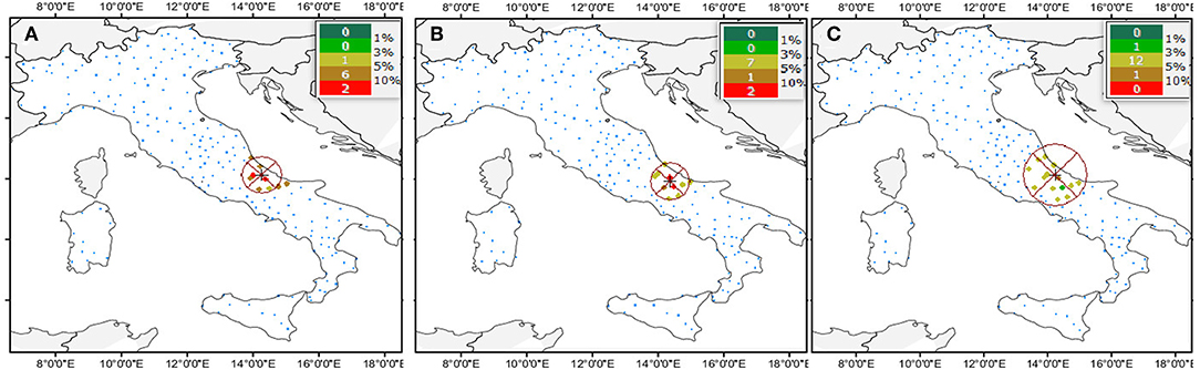
Figure 2. Isotropic neighboring circle for erosivity density during (A) August, (B) September, and (C) October. The colured bands in the corner represent the patterns of station-points inside of any neighboring circle with the related percentage weighted given for any data-points.

Trend analysis shows that only a weak gradient of the erosivity density data occurs along the northwest to southeast direction. The non-existence of a non-random (deterministic) component can be attributed to the persistent rainfall, which is received from the Atlantic. Based on this finding, the stationarity hypothesis cannot be rejected both locally and for the whole country.

Then, the implementation of the iterative procedure provides a satisfactory fit of covariance and cross-covariance models (Figure 3). This fit results from summing the geostatistical nugget and an exponential model with the previous estimated ranges of 50 km, for August and September, and 100 km, for October (solid curve in Figure 3, respectively). The obtained covariance and cross-covariance functions have been then used to train the geospatial tool on how control points act during the interpolation with LNPK. According to the isotropic neighborhood of data-points, five points per target-site have been used for estimation, corresponding to the search circle of the erosivity density-threshold (z_k = 3 MJ ha⁻¹ h⁻¹).

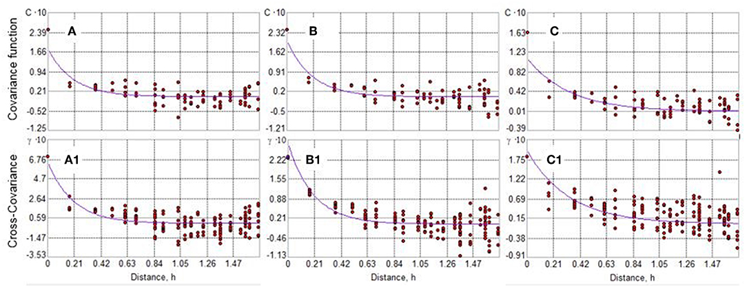
Figure 3. Covariance function C_X(h) at threshold z_k (ED>3 MJ ha⁻¹ h⁻¹) for (A) August, (B) September, and (C) October month, with respective model of co-regionalization between indicator and uniform transforms [cross-covariance CC_XI(h; z_k)], (a₁), (b₁), and (c₁).

More specifically, this exponential model assumes that, at the monthly scale, the range variations of the erosivity density threshold are associated with the storm characteristics and local geographical features. This suggests that the increasing variability of hydrological events produce a more regular pattern of spatial variation in October and a spot-mosaic pattern in August and September. These months suggest that an enhanced hazard is associated with complex, more localized storm events, characterized by a strong convective component. In addition, the nugget ratio is larger for the August month (0.073), than to the months of September and October (around 0.05). This represents the random (unexplained) variance caused by the inherent variability in the data, and the spatial variation at distance much shorter than sample spacing which cannot be resolved in August at the scale where sampling is performed (<20 km), or owing to some measurement errors.

Spatial Patterns of Erosivity Density Exceeding Threshold Values

As already reported in Ballabio et al. (2017), the most erosive months in Italy are August (in North Italy), September (in Central Italy) and October (in Southern Italy). This paper reports in Figures 4A,B the kriged probability maps exceeding the erosivity density threshold-value of 3 MJ ha⁻¹ h⁻¹ for the months of August and September, respectively. Our results extend the current knowledge about the hydrological risk prone areas highlighting as ca 65% of the Italian peninsula has a probability higher than 50% to be subjected to hydrological hazards in August. The severely affected hydrological prone areas hazard, in addition to Northern regions already reported by Ballabio et al. (i.e., Friuli-Venezia Giulia, Lombardy, Veneto and Emilia Romagna) are Central regions as Tuscany and Umbria. While Molise, Campania, Basilicata and parts of Sicily are moderately affected (Figure 4A). In the Mediterranean region, circumstances causing precipitation extremes, besides the inherent probability of higher data variance, are due to interaction/combination of different factors acting at local and large scales. Among these, the Mediterranean Sea Surface Temperature (SST), the moisture fluxes from North Atlantic, the orographic forcing factors, and the change of synoptic climatology in different seasons (Figures 4A,B). In particular the characteristic of the development and evolution of cyclones in the Mediterranean have both a smaller spatial and temporal scale than North Atlantic systems, with generally shorter life (Trigo et al., 1999). Our results have clearly highlighted the effects on the Italian peninsula, of this strong seasonal signal of the Mediterranean cyclones distribution during precipitation extremes.

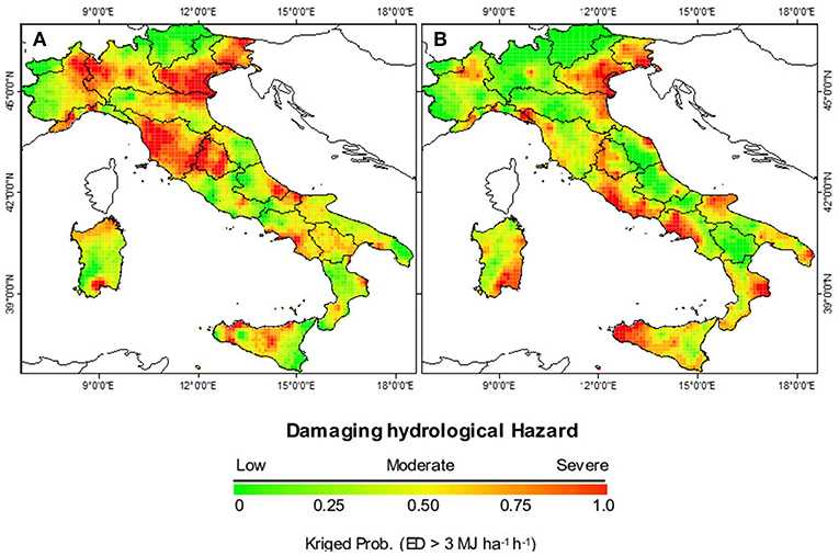
Figure 4. Spatial patterns of kriged-probability maps exceeding the erosivity density threshold-value z_k of 3 MJ ha⁻¹ h⁻¹ for (A) August and (B) September across Italy for the period 2002–2011.

In August, Figure 4A reports, over our peninsula, the effect of extreme precipitation events caused by pressure anomalies associated with conditions favoring intense North-Atlantic cyclones (i.e., the cyclogenesis pattern with the cyclone centered North-Western out of the coasts of Ireland and with the low extending south-eastward over the Gulf of Genoa affecting the Alpine region, Tuscany, Umbria regions and the Adriatic sea and the North-Eastern Coast of Sicily. While the extreme precipitation highlighted in September and October (Figures 4B, 5A) are associated to the Cyprus low (i.e., the cyclogenesis pattern common in the Mediterranean area during Autumn (SON) and Winter (DJF), which north-westward affects Sicily, Puglia, Ioanian Calabria, Campania and Latium and then the regions northward.

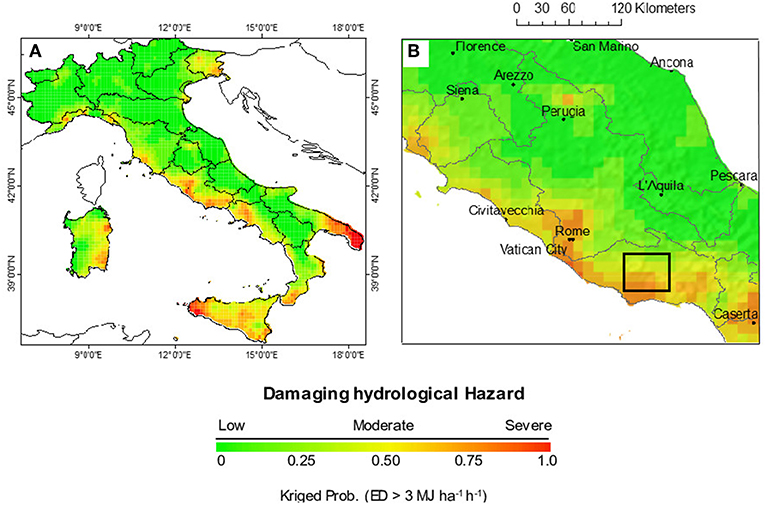
Figure 5. Spatial patterns of kriged-probability maps exceeding the erosivity density threshold-value z_k of 3 MJ ha⁻¹ h⁻¹ for (A), October across Italy for the period 2002–2011 and (B) zoomed area in Central Italy where boundaries of river basin and main cities are over-imposed. The rectangular shape indicates the area for which the perspective view of Figure 6 was made.

The characteristic depth of Cyprus cyclones, with enhanced (negative) geopotential height anomalies, the intensity (“depth”) and its location is the driving factor of the effect of visible heavy precipitations in autumns and winter (Maheras et al., 2002). The “depth” of a cyclone is the pressure difference between its center and periphery. Our results show this situation. In September, the area hit by storm erosive events (erosivity density >3 MJ ha⁻¹ h⁻¹) drops to around 50% of the peninsula. However, the probability of erosive events is still high in along the coastal and insular areas. Veneto, Westerly Umbria, some areas of Liguria, Tuscany and Campania coast still can face hydrological hazard in September (Figure 4B) but the effect of the cyclogenesis characteristics are evident in this month on the coasts and mainland of the Latium, Northern Campania, Puglia Garganica, Ionian Calabria, Sicily and Eastern Sardinia which all are facing higher hydrological hazard as consequence of the Northwestward exstension of the Cyprus Low.

October presents a smaller hydrological hazard, with areas prone to erosive events falling to about 30% of Italian territory; mainly located in the Campania coastal, Southern Basilicata, Sicily, Eastern Sardinia and Latium (Figure 5A).

Taking into account the whole period August-October, the regions Campania, Latium and Sicily are more affected than others. In particular, the months of August and September represent a vulnerable timespan of the year, where both storm are the most erosive and lands are bare. This combination drives to hydrological hazards events across to more than 50% of the Italian territory. Focusing in Latium region, we find that lower Tiber river basin of the Rome metropolitan area (Latina Province) is at a high hazard (Figure 5B). In particular, we can observe the Latina landscape (black square in Figure 5B) concerned in a 3-D view with the erosivity density threshold-value z_k of 3 MJ ha⁻¹h⁻¹ for the October month (Figure 6).

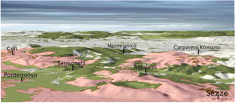
Figure 6. Spatial patterns of kriged-probability perspective view exceeding the erosivity density threshold-value z_k of 3 MJ ha⁻¹ h⁻¹ with probability >50% (pink color) for October across the Latina Province (Southern Latium) for the period 2002–2011. Wood areas are in green color.

The pink color area in this figure represents the zones where the 3 MJ ha⁻¹ h⁻¹ threshold value has a probability higher than 50%, and thus are the places mostly prone to damaging hydrological hazard at beginning of the autumn. These areas are included among the Villages of Cori, Pontenuovo, Sermoneta, Bassiano, Carpineto Romano and Sezze. This suggests several hydrological implications, which must be taken into account when, for instance, the effects of land use like urbanization and deforestation are examined, or when the relation between climate change and flash-flood occurrence is studied (Marchi et al., 2010).

Vulnerable timespan keeps is very active also for the Sicily island in the month of October. Sicily presents geo-climatic characteristics that make its territory prone to flash-flood, especially in September and October, as demonstrated by some recent events (Diodato and Bellocchi, 2010; Aronica et al., 2012; Fiorillo et al., 2016; Candela and Aronica, 2017). On the other hand, from the specific analysis of the extreme rainfall occurred in Sicily, it emerges that precipitations are nearly always associated with particularly intense storm (Caccamo et al., 2016). These finding agree with the results of Messeri et al. (2015), who showed the most perturbed flows in Italy, associated with the highest impact in terms of damaging hydrological events, are observed in autumn. These cyclonic perturbations tend to have short life cycles, with average radii in the range 300 to 500 km in this period of the year (Lionello et al., 2006), and a predominance of convective storms. Convective storms can have, however, smaller radii (around 10-50 km), as suggested by the small kriged-ranges obtained with the covariance functions. These are the highest erosive storms that may occur in major part of Italy, characterized by a complex property in transferring erosive energy to lands. In these localities, sub-grid scale convection and intensification phenomena dominate rain-producing processes (e.g. Mazzarella, 1999; Dünkeloh and Jacobeit, 2003), accompanied by several rain episodes releasing in a few hours as much energy as in an average year or more. These changes capture the shift toward autumn of some flash-flood conditions typical of summer (Gaume et al., 2009). Delayed effects show that the warmer Mediterranean period taking place from end-summer to early autumn is leading to more frequent and intense torrential rains (Millán et al., 2005).

Cross-Validation and Error Assessment

The results from the cross-validation and error assessment procedures check have been presented with joint statistical errors and as monthly scatter diagrams (Figures 7A–C). They show that the measured values of erosivity density are in agreement with the predicted probability indicators.

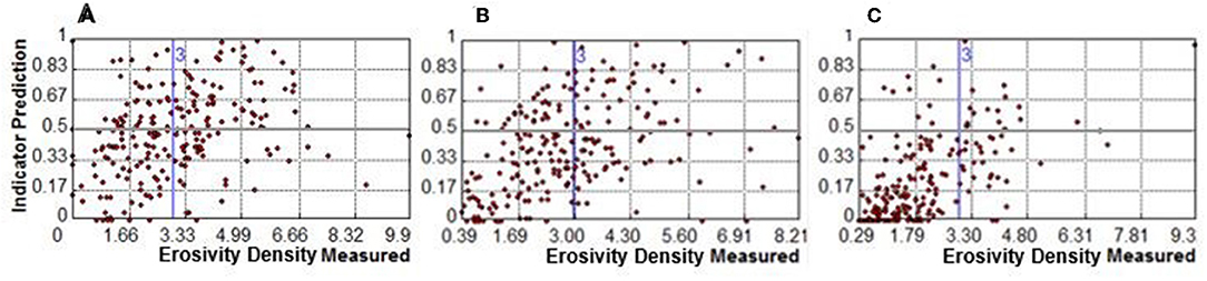
Figure 7. Scatterplot of cross-validation between storm erosivity measured and indicator probability kriging for the erosivity-thresholds z_k (ED>3 MJ ha⁻¹ h⁻¹), for (A) August, (B) September, and (C) October month. The blue vertical lines in both the graphs represent the respective ED thresholds, while the gray horizontal lines separate the kriged-prediction indicator with probability above 0.50 from those below 0.50.

In this way, mean values of 0.006 in August and September, and 0.01 in October, make evident that there is no systematic error because the root mean square error is close to the average standard errors. The mean thus correctly assesses the variability in predictions. In addition, the Root Mean Square Standardized (RMSS) error variance is the same and close the 1.0 as compared to the theoretical variance of the kriging variance.

At sub-regional scale, we performed a qualitative error assessment by comparing kriged-probability erosivity density >3 MJ ha⁻¹ h⁻¹ (Figure 8A) to previously published damaging hydrological risk maps (joint probability of landslides and floods, Figure 8B, Guzzetti et al., 2002) for the Sicily island.

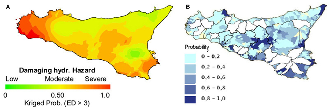
Figure 8. Comparison of (A) kriged probability for erosivity density (ED>3 MJ ha⁻¹ h⁻¹) for October with (B) damaging hydrological risk maps (joint probability of landslides and floods occurrence) with 5-years return period (Guzzetti et al., 2002) for the Sicily region.

The comparison of kriged probability erosivity density higher than the threshold (orange colors in Figure 8A) is in agreement with probability hydrological risk areas (blue colors in Figure 8B), except for the extreme westernmost part of the island. However, a strict parallelism between the two maps is not to be expected considering the multifaceted nature of the involved phenomena and the different time periods covered.

Conclusion

The widespread availability of high-temporal resolution rainfall records for large areas and the development of climate models opens new opportunities for using geostatistical methods for large scale planning and hazard prevention. This paper presents a geostatistical modeling framework, which uses a probabilistic approach to assess the spatial variability of storm erosivity density throughout the Italian regions. The results so obtained suggest the possibility of using geostatistical spatial modeling to determine the probability of exceeding high erosivity density thresholds and generate probability maps to delineate the most sensitive areas. These areas, highly vulnerable, may result in catastrophic regime shifts connected with the occurrence of damaging hydrological events. We offer the results of this work as a springboard to support policy-makers, local authorities and civil protection in planning actions, in the medium and long term, aimed at reducing hydrological disasters. In fact, such a soft-computing model represents a paradigm shift on how to provide timely, accurate and actionable hydrologic hazard information. Relying on credible information regarding erosivity density and its environmental drivers, this study shows how geostatistical methods can be practically implemented to create countrywide spatially explicit probabilistic maps capable to describe the seasonal effect of cyclogenesis‘ modification as the case of the highlighted seasonal variation of the North Atlantic and Cyprus Low systems during extreme events. These probabilistic maps can therefore be of great help in studying erosive hazards or the effects over Italy, of the generation and growth of Mediterranean cyclones, which however depends on the relationship of several factors among others, the complex orography, large scale air flow, and SST. In addition, these probabilistic maps refer not only to a possible check of the physical understanding of some processes, but also to the possibility to gain information where data or measurements actually do not exist. In fact, without giving the value in each point but returning a map of probabilities, this approach can support decision-making because it identifies the hydrologic danger associated with the probability to exceed an erosivity density threshold.

ED–outputs have the advantage to be developed based on more available data and can be scaled up for producing weather hazard maps. Vice versa, the disadvantage is that the same probability to overcome a specific ED threshold may have different meanings when superimposed to areas with different combinations of morphology, soil erodibility, land use, plant density, and management. In addition, these findings are purely geostatistical, with no explicit mechanistic modeling of erosivity density.

This study has also some limitations because it does not consider that population density, infrastructures, plant density, and other factors also influence the occurrence of a damage. In addition, the particularly prolonged low-intensity rainy periods, which can condition landslide fatalities, are not accounted in this probability calculation.

Data Availability Statement

The datasets generated for this study are available on request to the corresponding author.

Author Contributions

ND conceived the study, performed the analysis and drafted the manuscript with GB, who wrote the final manuscript. PB and PP prepared and organized the sediment data used in the study, and contributed to scientific discussion of the article together with CB.

Conflict of Interest

The authors declare that the research was conducted in the absence of any commercial or financial relationships that could be construed as a potential conflict of interest.

Acknowledgments

We thank the NTNU publishing fund support to cover article processing charges in Open Access Journals.

References

Allison, R. J., and Thomas, D. S. G. (1993). “The sensitivity of landscapes,” in Landscape Sensitivity, eds D. S. G. Thomas and R. J. Allison (Chichester: John Wiley & Sons), 1–5.
Arnell, N. W. (2011). Uncertainty in the relationship between climate forcing and hydrological response in UK catchments. Hydrol. Earth Syst. Sci. 15, 897–912. doi: 10.5194/hess-15-897-2011
Aronica, G. T., Brigand, G., and Morey, N. (2012). Flash floods and debris flow in the city area of Messina, north-east part of Sicily, Italy in October 2009: the case of the Giampilieri catchment. Nat. Hazards Earth Syst. Sci. 12, 1295–1309. doi: 10.5194/nhess-12-1295-2012
Ballabio, C., Borrelli, P., Spinoni, J., Meusburger, K., Michaelides, S., Beguería, S., et al. (2017). Mapping monthly rainfall erosivity in Europe. Sci. Total Environ. 579, 1298–1315. doi: 10.1016/j.scitotenv.2016.11.123
Bintliff, J. (2002). Time, process and catastrophism in the study of Mediterranean alluvial history: a review. World Archaeol. 33, 417–435. doi: 10.1080/00438240120107459
Borrelli, P., Diodato, N., and Panagos, P. (2016). Rainfall erosivity in Italy: a national scale spatio-temporal assessment. Int. J. Digit. Earth 9, 835–850. doi: 10.1080/17538947.2016.1148203
Brunsden, D. (2001). A critical assessment of the sensitivity concept in geomorphology. Catena 42, 99–123. doi: 10.1016/S0341-8162(00)00134-X
Caccamo, M. T., Cannuli, A., Castorina, G., Colombo, F., Insinga, V., Maiorana, E., and Magazù, S. (2016). Highlights on extreme meteorological events in Sicily. Geoscience 1, 78–87. Available online at: http://article.scirea.org/pdf/17005.pdf
Candela, A., and Aronica, G. T. (2017). Probabilistic flood hazard mapping using bivariate analysis based on copulas. ASCE-ASME J. Risk Uncertain. Eng. Syst. 3:a4016002. doi: 10.1061/AJRUA6.0000883
Cevasco, A., Diodato, N., Revellino, P., Fiorillo, F., Grelle, G., and Guadagno, F. M. (2015). Storminess and geo-hydrological events affecting small coastal basins in a terraced Mediterranean environment. Sci. Total Environ. 532, 208–219. doi: 10.1016/j.scitotenv.2015.06.017
Corella, J. P., Valero-Garcés, B. L., Vicente- Serrano, S. M., Brauer, A., and Benito, G. (2016). Three millennia of heavy rainfalls in Western Mediterranean: frequency, seasonality and atmospheric drivers. Sci. Rep. 6:38206. doi: 10.1038/srep38206
Curić, M., and Janc, D. (2011). Comparison of modeled and observed accumulated convective precipitation in mountainous and flat land areas. J. Hydrometeorol. 12, 245–261. doi: 10.1175/2010JHM1259.1
Dabney, S. M., Yoder, D. C., Vieira, D., and Bingner, R. (2011). Enhancing RUSLE to include runoff-driven phenomena. Hydrol. Process. 25, 1373–1390. doi: 10.1002/hyp.7897
De Luís, M., García-Cano, M. F., Cortina, J., Raventós, J., Gonzáles-Hidalgo, J. C., and Sánchez, J. R. (2001). Climatic trends, disturbances and short-term vegetation dynamics in a Mediterranean shrubland. For. Ecol. Manage. 147, 25–37. doi: 10.1016/S0378-1127(00)00438-2
Diakakis, M., Priskos, G., and Skordoulis, M. (2018). Public perception of flood risk in flash flood prone areas of Eastern Mediterranean: the case of Attica Region in Greece. Int. J. Disast. Risk Re. 28, 404–413. doi: 10.1016/j.ijdrr.2018.03.018
Diodato, N. (2005). Geostatistical uncertainty modelling for the environmental hazard assessment during single erosive rainstorm events. Environ. Monit. Assess. 105, 25–42. doi: 10.1007/s10661-005-2815-x
Diodato, N., and Bellocchi, G. (2010). Storminess and environmental changes in the Mediterranean Central Area. Earth Interact. 14, 1–16. doi: 10.1175/2010EI306.1
Diodato, N., Bellocchi, G., Chirico, G. B., and Romano, N. (2011). How the aggressiveness of rainfalls in the Mediterranean lands is enhanced by climate change. Clim. Change 108, 591–599. doi: 10.1007/s10584-011-0216-4
Diodato, N., Ljungqvist, C. F., and Bellocchi, G. (2019). A millennium-long reconstruction of damaging hydrological events across Italy. Sci. Rep. 9:9963. doi: 10.1038/s41598-019-46207-7
Downs, P. W., and Gregory, K. J. (1993). “The sensitivity of river channels in the landscape system,” in Landscape Sensitivity, eds D. S. G. Thomas and R. J. Allison (Chichester: John Wiley & Sons), 15–30.
Dünkeloh, A., and Jacobeit, J. (2003). Circulation dynamics of Mediterranean precipitation variability 1948-1998. Int. J. Climatol. 23, 1843–1866. doi: 10.1002/joc.973
Fiorillo, F., Diodato, N., and Meo, M. (2016). Reconstruction of a storm map and new approach in the definition of categories of the extreme rainfall, northeastern Sicily. Water 8:330. doi: 10.3390/w8080330
Foster, G. R., Toy, T. E., and Renard, K. G. (2003). “Comparison of the USLE, RUSLE1. 06c, and RUSLE2 for application to highly disturbed lands,” in First Interagency Conference on Research in Watersheds, eds K. G. Renard, S. A. McElroy, and W. J. Gburek (Washington, DC: US Department of Agriculture, Agricultural Research Service), 154–160.
Gaume, E., Bain, V., Bernardara, P., Newinger, O., Barbuc, M., Bateman, A., et al. (2009). A compilation of data on European flash floods. J. Hydrol. 367, 70–78. doi: 10.1016/j.jhydrol.2008.12.028
Goovaerts, P. (1997). Geostatistics for Natural Resources Evaluation. New York, NY: Oxford University Press.
Guzzetti, F., Cipolla, F., Lolli, O., Pagliacci, S., and Tonelli, G. (2002). An Information System on Historical Landslides and Floods in Italy. Urban Hazards Forum. New York, NY: John Jay College, CUNY.
Guzzetti, F., Peruccacci, S., Rossi, M., and Stark, C. P. (2007). Rainfall thresholds for the initiation of landslides in central and southern Europe. Meteorol. Atmos. Phys. 98, 239–267. doi: 10.1007/s00703-007-0262-7
Harris, R. M. B., Beaumont, L. J., Vance, T. R., Tozer, C. R., Remenyi, T. A., Perkins-Kirkpatrick, S. E., et al. (2018). Biological responses to the press and pulse of climate trends and extreme events. Nat. Clim. Change 8, 579–587. doi: 10.1038/s41558-018-0187-9
Homar, V., and Stensrud, D. J. (2004). Sensitivities of an intense Mediterranean cyclone: analysis and validation. Q. J. R. Meteorol. Soc. 130A, 2519–2540. doi: 10.1256/qj.03.85
Huggett, R. J. (1988). Dissipative systems: implications for geomorphology. Earth Surf. Process. Landf. 13, 45–49. doi: 10.1002/esp.3290130107
Johnston, K., ver Hoef, J. M., Krivoruchko, K., and Lucas, N. (2001). Using ArcGis Geostatistical Analyst. New York, NY: Environmental Systems Research Institute.
Journel, A. G. (1983). Nonparametric estimation of spatial distributions. J. Ass. Math. Geol. 15, 445–468. doi: 10.1007/BF01031292
Kayler, Z. E., De Boeck, H. J., Fatichi, S., Grünzweig, J. M., Merbold, L., Beier, C., et al. (2015). Experiments to confront the environmental extremes of climate change. Front. Ecol. Environ. 13, 219–225. doi: 10.1890/140174
Kinnell, P. I. A. (2010). Event soil loss, runoff and the universal soil loss equation family of models: a review. J. Hydrol. 385, 384–397. doi: 10.1016/j.jhydrol.2010.01.024
Knight, J., and Harrison, S. (2013). The impacts of climate change on terrestrial earth surface systems. Nat. Clim. Change 3, 24–29. doi: 10.1038/nclimate1660
Li, X., Meshgi, A., and Babovic, V. (2016). Spatio-temporal variation of wet and dry spell characteristics of tropical precipitation in Singapore and its association with ENSO. Int. J. Climatol. 36, 4831–4846. doi: 10.1002/joc.4672
Lionello, P., Bhend, J., Buzzi, A., Della-Marta, P. M., Krichak, S. O., Jansà, A., et al. (2006). “Cyclones in the Mediterranean region: climatology and effects on the environment,” in Mediterranean Climate Variability, eds P. Lionello, P. Malanotte-Rizzoli, and R. Boscolo (Amsterdam: Elsevier), 325–372. doi: 10.1016/S1571-9197(06)80009-1
Luterbacher, J., García-Herrera, R., Akçer-Ön, S., Zorita, E., Allan, R., Alvarez-Castro, M. C., et al. (2012). “A review of 2000 years of paleoclimatic evidence in the Mediterranean,” in Mediterranean Climate Variability, eds P. Lionello, P. Malanotte-Rizzoli, and R. Boscolo (Amsterdam: Elsevier), 87–185.
Maheras, P., Flocas, H. A., Anagnostopoulou, C., and Patrikas, I. (2002). On the vertical structure of composite surface cyclones in the Mediterranean region. Theor. Appl. Climatol. 71,199–217. doi: 10.1007/s007040200005
Marchi, L., Borga, M., Preciso, E., and Gaume, E. (2010). Characterisation of selected extreme flash floods in Europe and implications for flood risk management. J. Hydrol. 394, 118–133. doi: 10.1016/j.jhydrol.2010.07.017
Mazzarella, A. (1999). Multifractal dynamic rainfall processes in Italy. Theor. Appl. Climatol. 63, 73–78. doi: 10.1007/s007040050093
Mendoza, G. A., Anderson, A. B., and Gertner, G. Z. (2002). Integrating multi-criteria analysis and GIS for land condition assessment: part I - evaluation and restoration of military training. J. Geograph. Inform. Decision Anal. 6, 1–16.
Messeri, A., Morabito, M., Messeri, G., Brandani, G., Petralli, M., Natali, F., et al. (2015). Weather-related flood and landslide damage: a risk index for Italian regions. PLoS ONE 10:e0144468. doi: 10.1371/journal.pone.0144468
Meyer, K., Hoyer-Leitzel, A., Iams, S., Klasky, I., Lee, V., Ligtenberg, S., et al. (2018). Quantifying resilience to recurrent ecosystem disturbances using flow-kick dynamics. Nat. Sustain. 1, 671–678. doi: 10.1038/s41893-018-0168-z
Millán, M. M., Estrela, M. J., Sanz, M. J., Mantilla, E., Martin, M., Pastor, M., et al. (2005). Climatic feedbacks and desertification: the Mediterranean model. J. Clim. 18, 684–701. doi: 10.1175/JCLI-3283.1
Mulligan, M., and Wainwright, J. (2013). “Modelling and model building,” in Environmental Modelling, eds M. Mulligan, and J. Wainwright (Chichester: Wiley & Sons, Ltd), 7–26. doi: 10.1002/9781118351475.ch2
Panagos, P., Ballabio, C., Borrelli, P., Meusburger, K., Klik, A., Rousseva, S., et al. (2015). Rainfall erosivity in Europe. Sci. Total Environ. 511, 801–814. doi: 10.1016/j.scitotenv.2015.01.008
Panagos, P., Borrelli, P., Meusburger, K., Yu, B., Klik, A., Lim, K. J., et al. (2017). Global rainfall erosivity assessment based on high-temporal resolution rainfall records. Sci. Rep. 7:4175. doi: 10.1038/s41598-017-04282-8
Panagos, P., Borrelli, P., Spinoni, J., Ballabio, C., Meusburger, K., Beguería, S., et al. (2016). Monthly rainfall erosivity: conversion factors for different time resolutions and regional assessments. Water 8:119. doi: 10.3390/w8040119
Pereira, P., Oliva, M., and Baltrenaite, E. (2010). Modelling extreme precipitation in hazardous mountain areas: contribution to landscape planning and environmental management. J. Environ. Eng. Landsc. Manage. 18, 329–342. doi: 10.3846/jeelm.2010.38
Petrucci, O., Papagiannaki, K., Aceto, L., Boissier, L., Kotroni, V., Grimalt, M., et al. (2019). MEFF: the database of Mediterranean flood fatalities (1980 to 2015). J. Flood Risk Manage. 12:e12461. doi: 10.1111/jfr3.12461
Phillips, J. D. (2006). Evolutionary geomorphology: thresholds and nonlinearity in landform response to environmental change. Hydrol. Earth Syst. Sci. 10, 731–742. doi: 10.5194/hess-10-731-2006
Renard, K. G., Yoder, D. C., Ligtle, D. T., and Darney, S. M. (2011). “Universal soil loss equation,” in Handbook of erosion modelling, eds R. P. C. Morgan, and M. A. Nearing (Oxford: Wiley-Blackwell), 153–170.
Salvati, P., Petrucci, O., Rossi, M., Bianchi, C., Pasqua, A. A., and Guzzetti, F. (2018). Gender, age and circumstances analysis of flood and landslide fatalities in Italy. Sci. Total Environ. 610–611, 867–879. doi: 10.1016/j.scitotenv.2017.08.064
Seddon, A. W. R., Macias-Fauria, M., Long, P. R., Benz, D., and Willis, K. J. (2016). Sensitivity of global terrestrial ecosystems to climate variability. Nature 531, 229–232. doi: 10.1038/nature16986
Snyder, K. A., and Tartowski, S. L. (2006). Multi-scale temporal variation in water availability: implications for vegetation dynamics in arid and semi-arid ecosystems. J. Arid Environ. 65, 219–234. doi: 10.1016/j.jaridenv.2005.06.023
Sofia, G., Roder, G., Dalla Fontana, G., and Tarolli, P. (2017). Flood dynamics in urbanised landscapes: 100 years of climate and humans interaction. Sci. Rep. 7:40527. doi: 10.1038/srep40527
Srivastava, S. K. (2013). Threshold concepts in geographical information systems: a step towards conceptual understanding. J. Geograph. High. Educ. 37, 367–384. doi: 10.1080/03098265.2013.775569
Sullivan, J. (1984). Nonparametric estimation of spatial distributions (Ph.D. dissertation). Stanford University (unpublished).
Thomas, M. F. (2001). Landscape sensitivity in time and space - an introduction. Catena 42, 83–98. doi: 10.1016/S0341-8162(00)00133-8
Tobler, W. R. (1970). A computer movie simulating urban growth in the Detroit region. Econ. Geogr. 46, 234–240. doi: 10.2307/143141
Toy, T. J., Foster, G. R., and Renard, K. G. (2002). Soil Erosion: Prediction, Measurement, and Control. New York, NY: John Wiley & Sons, Inc.
Trigo, I. F., Davies, T. D., and Bigg, G. R. (1999). Objective climatology of cyclones in the Mediterranean region. J. Clim. 12, 1685–1696. doi: 10.1175/1520-0442(1999)012<1685:OCOCIT>2.0.CO;2
Trigo, R., Xoplaki, E., Zorita, E., Luterbacher, J., Krichak, S. O., Alpert, P., et al. (2006). “Relations between variability in the Mediterranean region and mid-latitude variability,” in Mediterranean climate variability, eds P. Lionello, P. Malanotte-Rizzoli, and R. Boscolo (Amsterdam: Elsevier), 180–226. doi: 10.1016/S1571-9197(06)80006-6
Wei, W., Chen, L. D., and Fu, B. J. (2009). Effects of rainfall change on water erosion processes in terrestrial ecosystems: a review. Prog. Phys. Geogr. 33, 307–318. doi: 10.1177/0309133309341426
Willmott, C. J., and Legates, D. R. (1991). Rising estimates of terrestrial and global precipitation. Clim. Res. 1, 179–186. doi: 10.3354/cr001179
Keywords: erosive density, hydrological hazard, prone area, geospatial probability map, Italy
Citation: Diodato N, Borrelli P, Panagos P, Bellocchi G and Bertolin C (2019) Communicating Hydrological Hazard-Prone Areas in Italy With Geospatial Probability Maps. Front. Environ. Sci. 7:193. doi: 10.3389/fenvs.2019.00193
Received: 03 September 2019; Accepted: 25 November 2019;
Published: 12 December 2019.
Edited by:
Víctor Orlando Magaña, National Autonomous University of Mexico, MexicoReviewed by:
Gabriele Buttafuoco, Italian National Research Council (CNR), ItalyStefano Federico, Italian National Research Council (CNR), Italy
Copyright © 2019 Diodato, Borrelli, Panagos, Bellocchi and Bertolin. This is an open-access article distributed under the terms of the Creative Commons Attribution License (CC BY). The use, distribution or reproduction in other forums is permitted, provided the original author(s) and the copyright owner(s) are credited and that the original publication in this journal is cited, in accordance with accepted academic practice. No use, distribution or reproduction is permitted which does not comply with these terms.
*Correspondence: Chiara Bertolin, chiara.bertolin@ntnu.no