Comparison of Neighborhood-Scale, Residential Property Flood-Loss Assessment Methodologies

Introduction and Background

Flood is one of the most damaging natural hazards, causing massive destruction to property, floodplain structures, and agricultural lands. National Severe Storms Laboratory (2021) recognizes five main types of flooding: 1) riverine, which occurs when excessive precipitation in the higher reaches of a watershed causes a stream to overflow its banks; 2) coastal, which is caused by high tides and/or onshore winds often exacerbated by heavy rainfall; 3) storm surge, associated with landfalling marine storms, often accompanied by strong winds and rain; 4) inland, in which persistent precipitation accumulates locally or a stream overflows due to an ice or debris jam or the failure of a dam or levee; and 5) flash, in which water rushes downslope during an intense local downpour, levee or dam failure, or sudden unclogging of an ice jam or debris blockage. Multiple types of floods may be occurring simultaneously in a given location, creating a compound flood, such as when high tides of coastal floods and storm surges are met by riverine floods from inland precipitation.

Approximately 99 percent of U.S. counties were affected by flooding of one or more of these types during the 1996–2019 period (FEMA 2021a). According to National Oceanic and Atmospheric Administration (National Oceanic and Atmospheric Administration, 2020), the 33 flood events in the U.S.A. from 1980 through 2020 that each caused more than $1 billion in damage (consumer price index- (CPI-) adjusted to 2020$) were responsible for a total of more than (CPI-adjusted) $151.2 billion in U.S. damage. Recent estimates suggest that perhaps three times more Americans (41 million) live within the 100-yr floodplain than suggested via Federal Emergency Management Agency (FEMA) flood maps (Wing et al., 2018).

Property loss (Mostafiz et al. 2020a; Mostafiz et al. 2020b)estimation from floods is important for assessing risk and therefore improving planning efforts to mitigate this hazard. However, such loss estimation from flooding is extremely complicated for several reasons. First, many components of loss must be considered, including direct losses such as to infrastructure, agriculture, and transportation, in addition to indirect, non-property losses such as missed work and productivity, and items of sentimental, non-quantifiable value. Second, many losses, particularly the uninsured losses, are uncatalogued. Third, because the different types of flooding (i.e., flash flooding, riverine flooding, storm surge flooding) include order-of-magnitude differences in the various types of losses, flood loss evaluation does not fall into a “one size fits all” methodology. As a result of these difficulties, despite the importance of having accurate and precise flood loss information, existing data are often inadequate and impossible to validate due to the lack of accurate empirical data.

Two major flood loss models – FEMA’s Hazus (Schneider and Schauer 2006) and U.S. Army Corps of Engineers (USACE) Hydrologic Engineering Center’s Flood Impact Analysis (HEC-FIA; Dunn 2000) – are widely used in the U.S.A. Another promising model – FEMA’s Flood Assessment Structure Tool (FAST; FEMA 2021b) – introduced in November 2019, is likely to become commonly used. Among the two leading flood models, FEMA’s Hazus, introduced in 1998 and now incorporating three “levels” of analysis based on the sophistication of input and output data (Figure 1), incorporates estimates of flood damage to structures, but also to agricultural and utility infrastructure, transportation networks, and other flood-related impacts. Hazus has been shown to be a valuable tool for flood adaptation planning (Banks et al., 2014) and has been used widely in recent years. Such applications include examining the advantages of levee setbacks (Dierauer et al., 2012), assessing feasibility of flood relocation (Cummings et al., 2012), cost-benefit analysis of floodplain conservation (Kousky and Walls 2014), evaluating potential for bridge scouring (Banks et al., 2016), comparing urban vs rural flood vulnerability (Remo et al., 2016), validating other flood estimation methods (Gutenson et al., 2018), estimating modern hurricane-induced flood damage in the context of historical hurricanes (Paul and Sharif 2018), determining impacts of sea-level rise (Ghanbari et al., 2020), and assessing community flood resilience (Allen et al., 2020). Sensitivity analysis on the various input functions in the flood component of Hazus has suggested that the choice of digital elevation data is important (Tate et al., 2015) and that the DDF, flood level, and restoration duration all affect model sensitivity (McGrath et al., 2015).

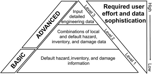
FIGURE 1. Schematic of information involved in each level of Hazus (modified from FEMA 2018).

HEC-FIA has also been used widely in the last two decades. Nafari (2013) elaborated on advantages and disadvantages of HEC-FIA for flood damage assessment. Prominent among the advantages of HEC-FIA software is the ability to incorporate quantitatively an estimation of consequences with uncertainty, thereby estimating and comparing the benefits of existing and future flood risk management measures (Lehman and Light 2016). HEC-FIA also has the advantage of providing separate estimates of direct economic, indirect economic, agricultural, and life loss consequences for flood hazards, by incorporating structure inventory, geospatially and externally derived flood depth grids, and depth-damage functions (DDFs; Lehman et al., 2014). An additional feature is HEC-FIA’s ability to incorporate information from other USACE software, such as the River Analysis System (HEC-RAS) for hydrograph-based or geographic information systems-based estimation of consequences for life and property (Dunn et al., 2016).

Prominent applications for HEC-FIA have been in dam safety (McClelland and Bowles 2002; Needham 2010) and other risk assessments. For instance, Mokhtari et al. (2017) used HEC-FIA to identify vulnerable buildings and croplands, and estimate property and crop losses, in the Ghamsar watershed of Iran for different flood return periods. HEC-FIA has also been used in recent years to predict storm surge impacts (Brackins and Kalyanapu 2016), compare the variation of loss using different sources of digital elevation models (DEM; Bhuyian and Kalyanapu 2018), and validate a new flood loss model (Gutenson et al., 2018).

While the major existing flood loss models are helpful, their utility is limited by three major factors which produce research gaps in the literature. First, at the macro-scale or in study areas with unavailable local input data, their accuracy relies on data from the national-level building inventory. For example, the National Structure Inventory (NSI; https://github.com/HydrologicEngineeringCenter/NSI) provides general information about individual buildings, such as number of stories, foundation type, first-floor height, building type, occupancy, building replacement cost, and content cost. However, data from NSI are incomplete and are often only estimated based on features observable from remote sensing. First-floor elevation is particularly important for assessing potential flood losses, but these building data sets fall short because they rely on Light Detection and Ranging (LIDAR) data that may be older and less accurate than more recently collected data at the micro-scale, particularly in areas that are subject to subsidence, such as Louisiana. Thus, improvements in estimation accuracy of flood loss requires more comprehensive input data at various spatial scales to enhance current understanding. The result is a research gap at the micro-scale. Data compiled from the Jefferson Parish (Louisiana) building inventory (JPBI; Jefferson Parish Geoportal 2021) is an example of a source that offers hope for improved loss estimates for individual buildings, if such collected data and other available data would be used in the flood loss models.

Several potential improvements to the national-level building inventories have gone underexplored, to date. One is the use of ground-truth data, such as Google Street View^® (GSV, https://earth.google.com/) and Zillow^® (https://www.zillow.com/) for input into flood loss models. GSV can be used to determine the number of stories and first-floor elevation perhaps more accurately than existing national-level building data sets. Likewise, Zillow, which provides information on number of stories, building square footage, property value, and other information, may allow for more accurate flood loss estimates. Both GSV and Zillow require visual interpretation of ground-based imagery to determine first-floor elevation and manual recording of building data. Finally, the 2019 National Building Cost Manual (NBCM; Moselle 2018) provides localized construction costs, which may assist in calculating building replacement cost of structures due to flood. Assembly of a “best available data” (BAD) database that includes information from these sources can enhance flood loss estimates and address this gap.

Another important component of flood loss modeling is accuracy and proper selection of the DDFs. Typically, a flood model includes a set of default (i.e., non-site-specific) DDFs, which are percentages of building (and, separately, content) damage as a function of flood depth in the building, with one default function for each combination of building inventory attributes (e.g., one-story residential building with no basement). All too often, users may run the flood loss estimation model with the default DDF without considering the implications of this “one size fits all” assumption, which can contribute to inaccuracies based on the quality of building inventory data upon which such a default DDF rests. Each DDF requires accuracy in the unique set of building attributes, so the appropriateness of the DDF selection depends on the type and accuracy of the data in the building inventory that must be input into the DDF calculation. The generalized set of default DDFs in the two leading models (i.e., Hazus (which uses the same set of default DDFs as FAST) and HEC-FIA) differ substantially from each other, even for the same building attributes (e.g., one-story, single-family, residential home with basement). A thorough examination of the sensitivity of estimated flood losses to the DDFs between the two leading models is lacking in the literature. While it is possible to overwrite the default DDFs when running either Hazus or HEC-FIA, it is difficult to know which DDFs to use in micro-scale analysis.

Another research gap regarding studies using the leading flood loss models is that they tend to ignore local idiosyncrasies because their purpose is usually to plan for and protect an entire county, state, or country. Yet variation within the spatial scale of analysis can be very important at the neighborhood or individual building scale. While there is a trend toward more spatially-integrated flood risk management in many countries (Bubeck et al., 2017), only a few comprehensive studies have evaluated the flood risk methodologies at the micro-scale, especially for individual buildings in a census block.

This study is motivated by the need to identify the effects of building features (i.e., building inventory), model selection, and the DDFs used in estimating building and content losses due to the flood hazard. The results of this study explore the extent to which the results of neighborhood-level Hazus, which has been widely used in flood studies, corresponds with the results from building-level FAST and HEC-FIA models. More specifically, the contribution and objectives of this research are to show the extent to which, at the neighborhood-scale:

1) a localized building inventory assembled from GSV, Zillow, a local parish (i.e., county)-level building inventory, and localized information from the 2019 NBCM differs from the national-level building inventory (i.e., NSI 2.0); the null hypothesis is no difference of means.

2) flood loss estimations differ among Hazus Level 2, FAST, and HEC-FIA, when all are using the same building inventory (i.e., NSI 2.0 or BAD) and DDF; the null hypothesis is no difference of means among the three.

3) improved, customized local building inventory information acquired in (1) above improves the within-model performance of Hazus Level 2, FAST, and HEC-FIA (separately) while using their respective default DDFs, over NSI 2.0; the null hypothesis is no difference of means.

4) the default DDFs in Hazus Level 2, FAST, and HEC-FIA produce different results from each other when they are switched among these three models with all keeping the same building inventory; the null hypothesis is no difference of means.

In general, the results call attention to model sensitivity to the input parameters and DDFs, which will aid in assessing vulnerability to losses in local flood planning and decision-making.

Materials and Methods

Study Area

Census block 220510220012004, in levee-protected, suburban Metairie, Louisiana, United States, which consists of 29 single-family residential dwellings (Figure 2), is selected for this analysis, for several reasons. First, Metairie is a densely-populated area that lies in a severe hazard area for flooding due to local rainfall that is expected to become more hazardous over time. Second, the availability of recently-collected flood depth grids at multiple return periods (i.e., 10-, 50-, 100-, 500-yr) for Metairie facilitates probabilistic analysis of the flood loss-return period relationship. Several flood and hurricane events in recent decades in this community have led to increasing amounts of flood mitigation spending and flood payouts each year (Coastal Protection and Restoration Authority (Coastal Protection and Restoration Authority (CPRA)) 2012; Taghi Nezhad Bilandi 2018), including many properties that have sustained repetitive flood losses (Ergen 2006; Mattei et al., 2009; Kick et al., 2011) on subsiding land (Zou et al., 2016). This census block is selected over other nearby census blocks because some part of it is expected to flood at every return period analyzed. Additionally, this census block is advantageous for study because it is bounded by easily identified roads, to ensure accuracy in analysis. Finally, the uniformity of building types (i.e., 100 percent residential, the subject of this study) offers ease of analysis because the same DDFs can be applied for the entire analysis.

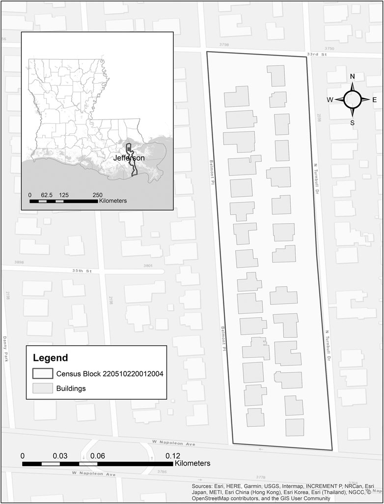
FIGURE 2. Study area census block in Jefferson Parish, Louisiana, with building footprint polygons and a gray rectangular dot in the index map.

Data

de Moel and Aerts (2011) noted that flood loss assessment requires input from four types of data: (1) magnitude of the flood hazard, which is provided by a flood depth grid; (2) land use type (e.g., residential, commercial, agricultural); (3) economic value of the object(s) of interest; and (4) DDFs, which, although not required, can improve data analysis over space. In practice, for property loss analysis, (2) and (3) above are often combined in a building inventory. Hazus, FAST, and HEC-FIA require these three components – flood depth grid, building inventory, and DDFs – to calculate the damage for an individual flood event (Table 1).

TABLE 1. Years analyzed and data sources, for property losses, by hazard in Louisiana.

Flood Depth Grid

Flood depth grids for four available return periods – 10-, 50-, 100-, and 500-yr – for Jefferson Parish, Louisiana, were developed at a scale of 3.048 m × 3.048 m, by FEMA through its Risk Mapping, Assessment and Planning (Risk MAP) program (FEMA 2021c). These data are input into all three models examined here (i.e., Hazus Level 2, FAST, and HEC-FIA). While the complexities associated with Risk MAP products have been identified (Johnson and Maloney 2011), these model-output data represent the best available input for understanding the flood risk.

Building Inventory

Building inventory consists of information about the fundamental features about each building, including, but not limited to, foundation height (first-floor height), foundation type, number of stories, square footage, building replacement cost, and content cost. The unavailability or inaccuracy of data regarding the building inventory variables listed above is among the most important barriers in flood loss studies (Taghinezhad et al., 2020a). Among the leading flood loss models, Hazus incorporates the General Building Stock (GBS) building inventory data set (Shultz 2017a) as the default input. FAST and HEC-FIA require input of building inventory data by the user.

Here, these data are considered from six sources (Table 2). The two national-level databases – GBS and NSI 2.0 – offer advantages of completeness but are disadvantageous because their accuracy is compromised where local-scale attributes might improve estimates of building damage. For example, use of GBS data has been observed to provide severe overestimates of replacement cost (Shultz 2017a), and the need for adjustment has been emphasized (Shultz 2017b). Furthermore, only five buildings in the study area are included in GBS, leading to further concerns that GBS may not represent the study area well.

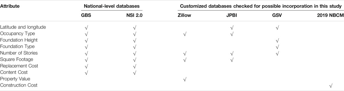
TABLE 2. Sources of attribute/data used in this study.

NSI is a structure-specific building dataset for the continuous United States. NSI 2.0 was developed from many sources, including Hazus, USACE, U.S. Geological Survey, National Center for Education Statistics, U.S. Census Bureau, Microsoft, Esri, and Homeland Infrastructure Foundation-Level Data (Barnett 2010). Availability of NSI 2.0 is typically limited to approved federal government applications and academic work such as this research. NSI 2.0 may prove useful, but its very recent release and its restricted availability leaves its utility largely untested.

Because of the uncertainty of NSI 2.0, this research collects and incorporates building attribute data not only for running FAST and HEC-FIA, but also for Hazus Level 2, for comparison between model runs using NSI 2.0 data vs that assembled from four local-level databases – Zillow, JPBI, visually-interpreted GSV imagery, and 2019 NBCM. These local-level sources may provide enhanced local-level accuracy but fail to include all of the variables needed for Hazus Level 2, FAST, and HEC-FIA. Therefore, an original data set named BAD is assembled here using the attribute data available from a compilation of each of these four data sets; the BAD is then input into the three models for comparison against runs using NSI 2.0 input data.

One of the four additional databases considered is Zillow, a popular web-based platform, typically used to identify property for sale and evaluate residential real estate attributes. The underlying data are accessible through the Zillow Transaction and Assessment dataset (ZTRAX), but in this research, data are collected manually through the web platform. Because the Zillow-reported property value combines the land and building value, and because some attribute data available from Zillow are incomplete and could be acquired elsewhere (Table 2) to assemble the BAD, ultimately it was decided that Zillow would not be used as a primary source in this study, but only to confirm data from other sources.

The other three data local-level databases are ultimately chosen for use in compiling BAD. JPBI is provided by the Jefferson Parish (Louisiana) Department of Floodplain Management & Hazard Mitigation. These data are useful because they are collected at the individual building level rather than being estimated en masse over a swath of properties. However, as shown in Table 2, the types of building attribute data available through JPBI are limited. GSV is another locally collected data source. Direct visual interpretation of GSV imagery is used to estimate occupancy type, number of stories, foundation type, and foundation height. Finally, the NCBM (Moselle 2018, p. 12) is used to collect construction cost per square foot. Thus, BAD is prepared by collating information from JPBI, GSV, and NBCM, with the data sources for each building attribute shown in Table 3. Zillow and GBS are also consulted to confirm data or resolve uncertainties.

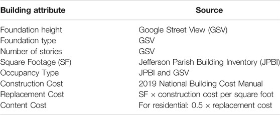
TABLE 3. Sources of best available data (BAD).

Depth-Damage Functions (DDFs)

Water depth relative to the first-floor elevation is the main variable in flood loss analysis (Taghinezhad et al., 2020b). Flood loss functions are used commonly to evaluate the percentage of loss to the building itself and (in a separate analysis) contents based on the flood depth variable (USACE 2003; Gulf Engineers & Consultants (Gulf Engineers and Consultants (GEC)) 2006). While the default DDFs for a given set of building inventory attributes are the same in Hazus and FAST, the default DDFs in HEC-FIA for the corresponding set of building inventory attributes differ substantially from those of the other models, as shown in the example of a one-story building with no basement in Figure 3. Moreover, Hazus (but not FAST) offers alternative DDFs that the user can select to match the suggested DDF for that set of building attributes. In addition, in any of the three models, the user can input any DDF, even if it is not among the suggested alternatives, for use in flood loss estimation.

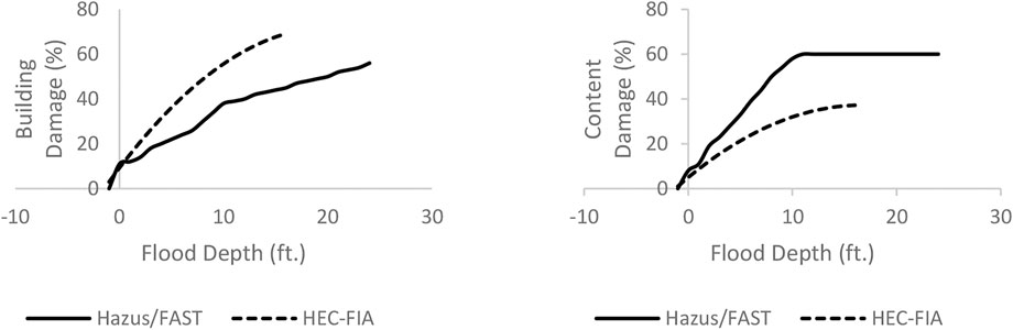
FIGURE 3. Comparison of default depth-damage curves for building (left panel) and contents (right panel), used in Hazus/FAST and HEC-FIA, for a one-story building with no basement.

Methodology

To address the four objectives, several combinations are tested against each other, with the following naming convention used. Building inventory ($I$) is specified as $I1$ for NSI 2.0 and $I2$ for BAD. The model/software ($S$) is represented as $S1$ for Hazus Level 2, $S2$ for FAST, and $S3$ for HEC-FIA. The input $DDF$ is denoted by $DDF1$ for that provided by Hazus Level 2 and FAST, and by $DDF2$ for that provided by HEC-FIA. The damage/loss ($L$) is designated as $L1$ for building and $L2$ for content. Finally, flood depth ($D$) is shown as $D1$ for 10-yr, $D2$ for 50-yr, $D3$ for 100-yr, and $D$4 for 500-yr flood return period.

Building Inventory Comparison

Within each of the six features in the building inventory comparison (i.e., foundation height, foundation type, number of stories, square footage, building replacement cost, and content cost), all combinations of options are examined comparatively, in this all-residential census block. Regarding the first feature – foundation height, the general egress requirements of the International Building Code (Ching & Winkel 2018) stipulate that stair risers in residential uses are to be built to a height between 4 and 7.75 inches. Because construction using maximum rise is more cost- and space-efficient, here a stair rise near that of the maximum allowed – 7.5 inches – is assumed for calculating FFE. Foundation height is calculated from GSV by multiplying 7.5 inches by the number of stairs. The difference between foundation heights from NSI 2.0 ($I1$) and BAD ($I2$) is examined at the neighborhood (census block) scale using pairwise t-test.

The second feature of the building inventory is foundation type. Because foundation type is a nominal-level variable (e.g., slab, crawl-space, pier-and-beam), non-parametric chi-square tests of independence are used to test the null hypotheses of no relationship between foundation types in $I1$ vs $I2$. The third feature – number of stories – is available from JPBI, but GSV is used to compile the BAD data set because it is more accurate and visible, making the data verifiable. This variable also requires the non-parametric chi-square test because it is of ordinal level. The null hypothesis is of no relationship between number of stories in $I1$ vs $I2$. Building area (square footage) is the fourth feature to be considered. Although square footage can be calculated from the JPBI shapefiles, it is not possible to calculate areas for multiple-story buildings. Therefore, square footage data from JPBI is used here to prepare BAD. The difference between square footage from $I1$ and $I2$ is examined at the neighborhood scale using pairwise t-test.

The building replacement cost using BAD is calculated by multiplying the per-square-foot construction cost from 2019 NBCM by the building area from JPBI. Because the average cost of constructing a single-family residence of average standard quality class in the New Orleans area is two percent higher than the national average (Moselle 2018, p. 7), construction costs used in the calculations here are increased by 2.0 percent over the values suggested in NBCM. Zillow was considered but ultimately is not used in this analysis, as it reports land value as part of the home purchase price. The difference between the building replacement cost from $I1$ and $I2$ is examined at the neighborhood scale using pairwise t-test.

Finally, content cost must be considered. In the NSI 2.0 data set, content cost is assumed to be equal to the building replacement cost. However, NSI 2.0 includes not only residential structures, but also commercial and industrial facilities that are likely to contain very expensive and abundant equipment and merchandise. Because this research includes only residential buildings in a relatively modest neighborhood where expensive jewelry and other possessions are likely to be minimal and vehicles are situated outside of the structure, it is assumed here that content cost is half of the building replacement cost. This assumption is supported by Hazus manual guidelines for similar situations (FEMA 2013, pp. 6–9). The difference between content cost from $I1$ and $I2$ is examined at the neighborhood scale using pairwise t-test.

Model Selection Sensitivity

To test the hypothesis resulting from Objective 2, the null hypothesis of equality of population mean (µ; used when the data are distributed normally, as indicated by a Shapiro-Wilk normality test) from among the three software/models,

is examined, again at the neighborhood scale (Eq. 1). To test this hypothesis, the values of all variables input (i.e., flood depth, DDF, and building inventory) are the same across model runs, if that variable is mandatory or optional for the given software. However, as is shown in Table 4, some variables are not eligible to be included in some of the software. Thus, any differences in building and/or content loss resulting from each model output would be attributable to differences in the structure information requirements and/or algorithms used in the three software modules. It should be noted that even though some additional variables are optional for input into one or more of the models (e.g., demographic data, vehicle type, fatalities), such variables are ignored in this analysis because they are deemed to be only indirectly related to building/content loss. The sections that follow provide an overview of how each of the three models is run.

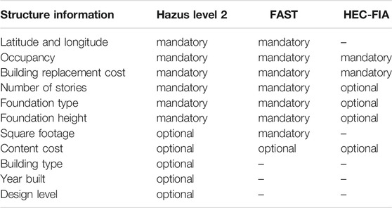
TABLE 4. Structure information used in the testing of software, and their categorization as mandatory or optional.

Hazus Level 2 analysis conducted in this study relies on user-input depth grids and user-defined building inventory rather than the system-generated flood conditions (see again Table 1). The first step is the generation of the study area (i.e., census block level). Then, the 10-yr flood depth grid is uploaded as user data. Next, the building inventory (NSI 2.0 or BAD) is imported under “User Defined Facilities (UDF).” Then, a new hazard scenario is created with the flood depth grid specified, and the riverine floodplain is delineated for a single return period using the default cell size (3.048 m × 3.048 m). This process is repeated for the 50-, 100-, and 500-yr flood depth grids to obtain the results. The DDF can be modified from the “damage functions” on the “analysis” tab.

FAST, which requires Anaconda for Python and the Hazus Python package (HazPy), offers improvements over Hazus Level 1, 2, and 3 in ease of use and processing efficiency. For example, only flood depth grid(s) (in .tiff format) and the structure attributes/table (.csv) are needed as input. Moreover, Hazus DDFs/curves are invoked automatically to calculate the flood loss. A complete explanation of using FAST for flood hazard assessment analysis is given at https://github.com/nhrap-hazus/FAST, but a brief overview to allow for replicability of our method is provided below.

After downloading the “FAST-master” folder from Github™ (https://github.com/nhrap-dev/FAST), the structure table (.csv), consisting of the mandatory fields of occupancy type, building replacement cost, building content value, number of stories, foundation type, first-floor height, total area of building, latitude, and longitude is built. Then, with the structure table moved into the “UDF” folder and the flood depth grids (.tiff) of interest (in the World Geodetic System 1984 (WGS84) projection) into the “rasters” folder, the “FAST.py” icon is executed. “Browse to Inventory Input (.csv)” is selected to input the structure inventory (.csv). Finally, the “Coastal Flooding attribute” is set to “riverine,” with the appropriate return period in the “depth grid” box. After “executing,” the output then appear in the “UDF” folder in .csv format. The DDF of building and contents can be modified from the “lookuptables” folder.

To use HEC-FIA, the layer files (i.e., study area boundary of the selected census block, NSI 2.0 data for the census block(s) of interest) are first converted into shapefiles. Likewise, all raster files (i.e., DEM and flood depth grids) are converted into Tag Image File Format (TIFF or TIF), and all shapefiles and raster files are assigned the same geographic projection system (WGS 1984 UTM Zone 15N).

For risk assessment, after creating and naming a “new study,” “add map layer” is selected from the “map layers” folder, and shapefiles are added (i.e., the study area and NSI 2.0 data). Then, “add terrain model” is selected under the “terrain grids” folder, and the DEM data are “imported.” Next, a new “watershed configurations” is created using the terrain grid (i.e., DEM) that was added. Then, the study area is imported in the “boundaries” and “impacted areas” folders separately, under “geographic data,” choosing from “shapefile name.” Under the “inundation data” folder, “new” is selected and the 10-, 50-, 100-, and 500-yr flood inundation configuration is created separately choosing “grid only” under the “hydraulic data type” and “inundation grid” under “grid only” with the watershed configuration created earlier. Then, “define event” is selected for each flood inundation configuration. The DDFs are imported using the “import from default” option under the “structure occ. types” folder. Next, “structure inventories” is selected, along with “generate from point shapefile” (i.e., NSI 2.0), and “use terrain+foundation height” is chosen under the “first floor elevation source” header. Then, the appropriate “shapefile fields” that were added from NSI 2.0 (i.e., “fd_id,” “st_damcat,” “occtype,” and “val_struct”) are uploaded into the “structure ID,” “damage category,” “occupancy type,” and “replacement value” inventory fields, respectively. Under “optional data” the following inventory fields are selected: “content value,” “foundation height,” “foundation type,” and number of stories,” and the following corresponding shapefile fields are selected: “val_cont,” “found_ht,” “found_type,” and “num_story.” Then, the “new” option is selected within the “alternatives” folder. The study area is clicked in the “impact area set” line, and the appropriate flood depth of interest is chosen for the “inundation configuration,” and NSI 2.0 is selected for the “structure inventory.” In the “simulation” folder, “new” is chosen, and the appropriate flood return period is selected in the “alternative” and “event” fields, with the output sent to the filename specified in the “name” line. Finally, the “compute” option is selected by clicking on the name given to the simulation in the previous step. The results show the aggregate and individual building damage reports, including both structure and content separately, for the selected census block. The DDF can be modified from the “structure occ. types” in the “structure inventories” under the “inventory” folder.

Building Inventory Sensitivity

To address Objective 3, the sensitivity of building inventory (NSI 2.0 vs BAD) is examined at the neighborhood scale, changing only the building inventory while leaving the model (i.e., Hazus Level 2, FAST, or HEC-FIA), loss type (i.e., building or content), and flood depth by return period (i.e., 10-, 50-, 100-, or 500-yr depth) the same, with default model DDF in each comparison, as described by the Eq. 2:

DDF Sensitivity

To address Objective 4, the sensitivity of DDFs is examined, changing only the depth damage function while leaving building inventory (i.e., NSI 2.0 or BAD), the model (i.e., Hazus Level 2, FAST, or HEC-FIA), loss type (i.e., building or content), and flood depth by return period (i.e., 10-, 50-, 100-, or 500-yr depth) the same in each comparison, as described by the Eq. 3:

Results

Building Inventory Comparison

A total of 28 residential buildings are reported in NSI 2.0, with 29 reported in JPBI and in GSV, in census block 220510220012004. Both in the NSI 2.0 and GSV data, all the buildings are classified as “single family dwelling,” but in JPBI, all buildings are showing the same occupancy type except one (Building ID 457824), which appears as “miscellaneous.” A summary/comparison of the six major variables in the building inventory by data source is shown in Table 5.

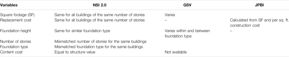
TABLE 5. Comparison of NSI 2.0, GSV, and JPBI data for the same neighborhood (census block 220510220012004).

As shown in Table 5, NSI 2.0 reports the same foundation height for all buildings in the study area with the same foundation type. Mean foundation height is 1.97 feet in NSI 2.0 and 2.17 feet in BAD, with ranges from 1.0 to 4.0 feet and from 0.6 to 5.6 feet in NSI 2.0 and BAD, respectively. Because the difference between the foundation height from NSI 2.0 vs BAD is not normally distributed (p-value = 0.028 using the Shapiro-Wilk normality test), the paired samples Wilcoxon test (also known as the Wilcoxon signed-rank test) is used instead of the paired t-test. That test suggests that there is no significant difference in median between the foundation height based on $I1$ vs $I2$ (p-value = 0.864). However, at the individual building scale, some substantial differences exist, as 50 percent of the buildings (i.e., 14 out of 28) have a difference of at least one foot in foundation height (Appendix A1).

NSI 2.0 shows 19 slab, eight crawlspace, and one basement foundation buildings, while BAD reports 20 slab and nine crawl foundation buildings (Appendix B1). Importantly, the two building inventories do not agree on the foundation type, as the chi-square tests of independence reveal no relationship between the foundation type as reported in NSI 2.0 vs BAD (p-value = 0.684). At the individual building scale, 39.29 percent of the building foundation types (11 of 28) differ between NSI 2.0 and BAD (Appendix B1).

Surprisingly, and seemingly a sign of inaccuracy of NSI 2.0, the chi-square test detects no relationship between the number of stories as reported by NSI 2.0 vs BAD (p-value = 1.0). At the individual building scale, 39.29 percent of the homes (11 out of 28) have an inconsistent number of stories reported in NSI 2.0 vs GSV (Appendix C1). Only two buildings have an inconsistent number of stories reported in JPBI vs GSV (Appendix C1). GSV and JPBI show 23 one-story and six two-story buildings whereas NSI 2.0 reports 19 one-story and nine two-story buildings (Appendix C1).

As described in Table 5 and shown in Appendix D1, NSI 2.0 reports the same square footage for all buildings in the study area with the same number of stories. Mean square footage is 1,517 in NSI 2.0 and 2,202 in BAD, with ranges from 1,148 (one-story) to 2,296 (two-story) and from 1,490 to 3,458 in NSI 2.0 and BAD, respectively. The difference in square footage between NSI 2.0 and BAD is normally distributed (p-value = 0.549 using the Shapiro-Wilk normality test), and the paired t-test for difference of means suggests a significant difference in mean area of buildings as reported by NSI 2.0 vs BAD (p-value < 0.001). At the individual building scale, NSI 2.0 estimates a smaller building area than BAD, especially for one-story buildings, but BAD is likely to be more accurate because of its dependence on JPBI data. BAD reports a greater square footage in 82.14 percent of the buildings (23 of 28; Appendix D1). Also, in 82.14 percent of the cases (23 out of 28), the difference in square footage between the two data sources exceeds 25 percent (Appendix D1), though this is for only 22 of the same 23 buildings as had been reported as having a greater square footage.

NSI 2.0 reports the same building replacement cost for all buildings in the study area with the same number of stories (Table 5). The mean building replacement cost is $108,588 and $199,781 in NSI 2.0 and BAD (respectively), with ranges from $77,265 to $186,924 and from $146,950 to $293,037 in NSI 2.0 and BAD, respectively. The difference in replacement cost between NSI 2.0 and BAD is normally distributed (p-value = 0.392 using the Shapiro-Wilk normality test), and the paired t-test suggests a statistically significantly lower mean building replacement cost (p-value < 0.001) calculated using NSI 2.0 vs BAD. At the individual building scale, NSI 2.0 estimates a lower building replacement cost than 2019 NBCM for 92.85 percent of the buildings (26 of 28), with 19 of these 26 having NSI 2.0-estimated building replacement cost at least 65 percent lower than that based on NBCM (Appendix E1).

Because NSI 2.0 reports the content cost equal to the building replacement cost (Table 5), content cost is assumed to be the same for all buildings in the study area with the same number of stories. The mean building content cost is $108,588 in NSI 2.0 and $99,890 in BAD, with ranges from $77,265 to $186,924 and from $73,475 to $146.518 in NSI 2.0 and BAD, respectively. The difference in content cost between NSI 2.0 and BAD is not normally distributed (p-value = 0.005 using the Shapiro-Wilk normality test), and the paired samples Wilcoxon test suggests that there is no significant difference in median between the content cost based on $I1$ vs $I2$ (p-value = 0.902). At the individual building scale, however, NSI 2.0 produces lower content cost estimates than BAD for one-story buildings, but because NSI 2.0 simply doubles the estimate for two-story buildings as compared to one-story, NSI 2.0 generates higher content cost estimates than BAD for two-story buildings, assuming all other building inventory variables are the same. For 68.85 percent of the cases (19 of 28), the difference in content cost between the two building inventories exceeds 20 percent (Appendix F1).

Model Selection Sensitivity

Because neither building nor content loss estimates are distributed normally for either NSI 2.0-or BAD-generated values (Table 6), and one-way ANOVA tests are appropriate only for normally distributed data (Burt et al., 2009), a Kruskal-Wallis test (Burt et al., 2009) is implemented to test model selection sensitivity. Results suggest that when using NSI 2.0 data, there is no significant difference in the median of building loss ($L1$) and (in a separate analysis) content loss ($L2$) among runs of Hazus Level 2, FAST, and HEC-FIA ($S1$, $S2$, and $S3$, respectively), holding DDF and flood return period constant, regardless of which DDF and return period are selected (Table 7). Likewise, use of BAD generates the same result – no significant difference in median of building loss or of content loss (Table 7).

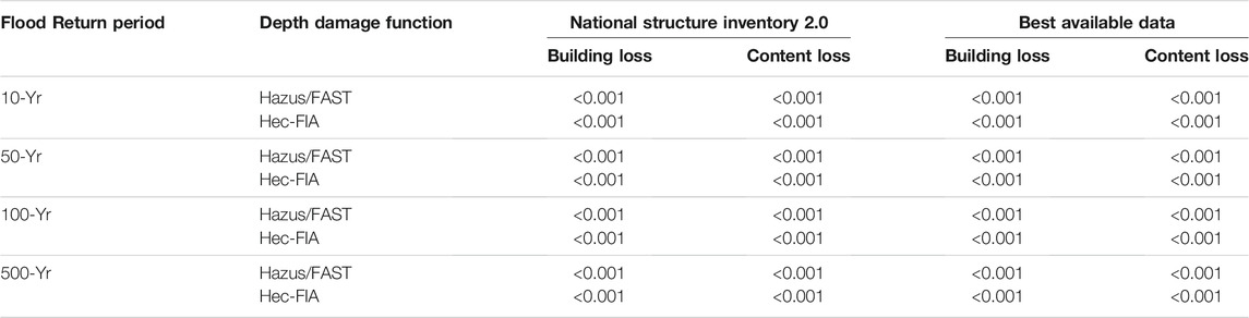
TABLE 6. p-values of Shapiro-Wilk normality test (with values <0.05 representing a non-normal distribution) of model sensitivity among Hazus Level 2, FAST, and HEC-FIA.

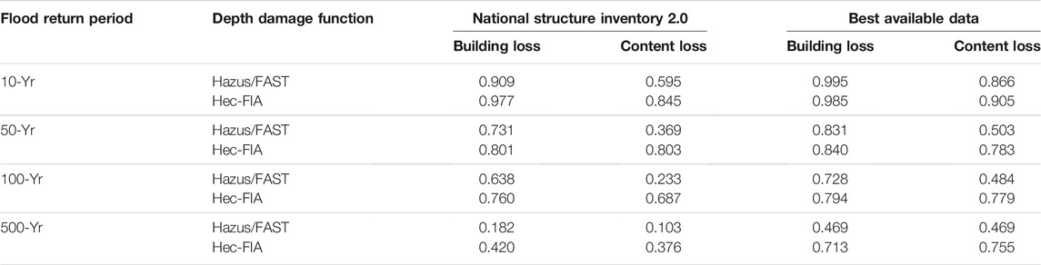
TABLE 7. p-values of Kruskal-Wallis test (with significant differences at p < 0.05 denoted by an asterisk) on difference of medians of building and content losses (separately) calculated by Hazus Level 2, FAST, and HEC-FIA, holding return period, building inventory, and depth-damage function constant.

However, at the individual building scale while using the same building inventory data to the extent possible (see again Table 4), the software selection may cause building and (in a separate analysis) content loss to differ in the case of some buildings (Appendix G1-G8).

Building Inventory Sensitivity

The building inventory sensitivity analysis quantifies the impact of the building inventory selection (NSI 2.0 vs BAD) for building and content loss using the three models (Hazus Level 2, FAST, and HEC-FIA) by flood return period (10-, 50-, 100-, and 500-yr) using the default DDF for that model. Most of the combinations of model and flood return period produce a non-normal distribution (Table 8, Columns 3 and 4). Thus, both non-parametric (paired samples Wilcoxon) and parametric (pairwise t-test) tests are implemented on the comparison of the median (for the non-parametric test) or mean (for the parametric test) building and content loss by building inventory, for the various combinations of models and return periods. The results are largely the same regardless of whether the paired samples Wilcoxon (Table 8, Columns 5 and 6) or pairwise t-test (Table 8, Columns 7 and 8) are used. Specifically, there are significant differences for all models and return periods regarding building loss, but no significant differences in median (or mean) content loss for any of the three models over any of the four flood return periods (Table 8).

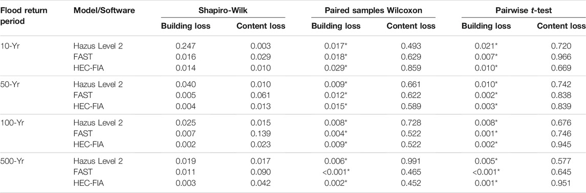
TABLE 8. p-values of Shapiro-Wilk normality test (with values <0.05 representing a non-normal distribution) for the distribution of differences between NSI 2.0- and BAD-generated loss estimates (for building and content, separately), and paired samples Wilcoxon and pairwise t-test (with significant differences at p < 0.05 denoted by an asterisk) of the difference between NSI 2.0- and BAD-generated losses.

Despite these results for the difference of medians/means between the two building inventories, building and content losses at the individual building scale tell a different story (Appendix H1-H6).

DDF Sensitivity

Running a flood loss estimation model for each of the 29 buildings after inputting another model’s default DDF for each building’s unique set of building inventory attributes can produce substantially different loss estimates (for both building and content loss) from those produced when the original model is run using its own default DDF for each building. Building and content losses for some combinations of building inventory and return period produce non-normal distributions (Columns 3 and 4 of Tables 9–11). Therefore, both the paired samples Wilcoxon and pairwise t-test are implemented on the comparison of the mean building and content loss by DDF, for the various combinations of building inventory and return period. Median or mean loss estimates using Hazus Level 2 (which has the same as the default DDF as used in FAST) vs HEC-FIA default DDFs of building loss and (in a separate analysis) content loss while running Hazus Level 2 model indicate some significant differences by building inventory (NSI 2.0 and BAD) and flood depth return periods (Table 9, Columns 5 through 8). The most significant differences are for building loss at higher flood return periods (i.e., 50-, 100-, and 500-yr), but with no significant difference at a 10-yr return period. Significant differences exist in the median and mean content loss (L2) at all combinations of building inventory and return period (Table 9, Columns 5 through 8).

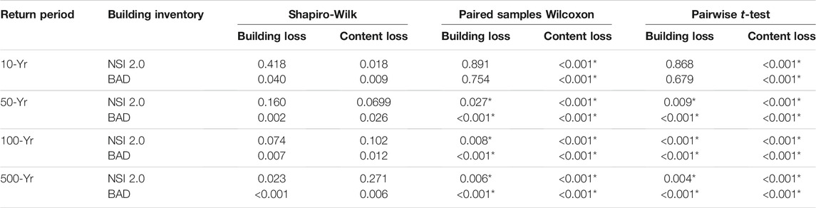
TABLE 9. p-values of Shapiro-Wilk normality test (with values <0.05 representing a non-normal distribution) for the distribution of differences between NSI 2.0- and BAD-generated building and content losses, and paired samples Wilcoxon and pairwise t-test (with significant differences at p < 0.05 denoted by an asterisk) of default DDF in Hazus Level 2 (which is the same as the default DDF in FAST) vs HEC-FIA as input in the Hazus Level 2.

Running FAST gives similar results to running Hazus Level 2 regarding DDF sensitivity. For building loss estimates, the FAST default DDFs provide different loss estimates than when FAST is run while overwriting HEC-FIA’s default DDFs for the corresponding set of building attributes. Statistically significantly different building loss estimates result from runs using the DDFs at the 50-, 100-, and 500-yr return periods, for both NSI 2.0 and for BAD building inventories. (Table 10, Column 5). At a 10-yr flood depth, no significant differences in DDF for building losses are observed (Table 10, Column 5). Regarding mean content loss (L2), a significant difference exists at all combinations of building inventory and return period (Table 10, Columns 6 and 8).

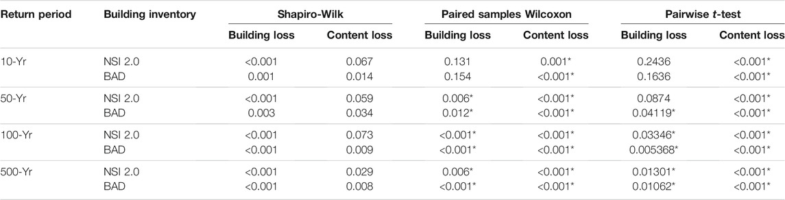
TABLE 10. As in Table 9, but for input in the FAST.

Running HEC-FIA gives the same statistical test results as running FAST, regarding DDF sensitivity for both building and content losses (Table 11). Moreover, all three models give the same result regarding content losses (Tables 9–11). At the individual building scale the DDF selection may cause building and (in a separate analysis) content loss to differ for all buildings (Appendix I1-I12).

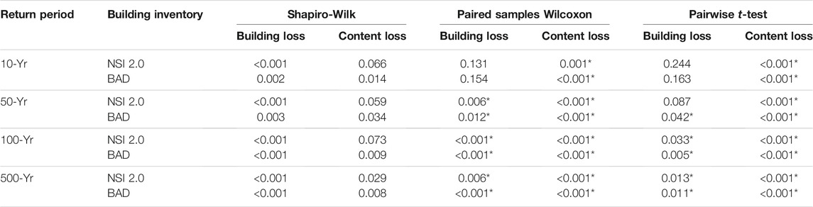
TABLE 11. As in Table 9, but for input in the HEC-FIA.

Discussion

Building Inventory Comparison

Even though the use of BAD seems to offer no improvement over NSI 2.0 in community-scale analysis of building and content loss (as evidenced by the lack of significant difference between the medians in foundation height), the variability in the data sets (i.e., NSI vs BAD) can make a major difference for individual homeowners when determining their vulnerability to flood losses (Appendix A2). Intuitively, the foundation height would seem to have the greatest impact on building/content loss from among the six variables that compose the building inventory. Thus, community-level planners may not see major differences in the two input data sets, as they are concerned with the aggregate impact (for which there is no difference of medians in the two data sets vis-à-vis foundation height). However, an individual homeowner should be cautious about the selection of input data set regarding foundation height.

Because of the low elevation and relief of the study area and the proclivity for flooding, there are no residences with a basement foundation in the study area or in coastal Louisiana. Yet the NSI 2.0 dataset reports that one of the 28 buildings (Building ID 455494) has a basement; this is likely an example of spurious data. Because the software-selected DDF to be used to calculate building and content flood loss for a given building is based on occupancy type, foundation type, and number of stories, an erroneous foundation type could possibly cause a substantial error in building and content DDF, which could theoretically give an inaccurate estimate of building and content loss (Appendix B2; Building ID 455494). However, only the presence or absence of a basement seems to matter in the calculation of building and content losses for any return period, as shown in Appendix B2 for the 500-yr flood return period.

While it may seem surprising that the NSI 2.0 and BAD report so many differences in number of stories, this result likely occurs because NSI 2.0 incorrectly counts some elevated one-story homes as two-story, based on LIDAR-collected local elevation differences. Because the set of DDFs for a building is based on foundation type, number of stories, and occupancy type, an erroneous number of stories can cause an incorrect building and content DDF to be used, thereby estimating building and content loss inaccurately (Appendix C2).

The building replacement cost as estimated in BAD is a function of square footage and per square foot construction cost, and content cost is half of the building replacement cost in BAD. Therefore, erroneous square footage information will cause errors in estimation of replacement and content cost, which can in turn lead to inaccurate estimation of building and content damage by flood (Appendix E2 and F2).

The statistically significantly lower estimate of the building replacement cost by NSI 2.0 as compared to BAD has several important implications. First, because the building replacement cost is a key player (along with DDF and flood depth) in determining building loss, inadequate estimates can have important consequences for both the homeowner and for actuarial interests. One potential discrepancy is the erroneous assumption in NSI 2.0 that all homes in the study area that have the same number of stories also have the same area and building replacement cost. By contrast, BAD considers the area and building replacement cost independently from the number of stories, potentially yielding a better estimate. However, further, detailed research at the individual building scale is needed to identify with certainty that BAD provides more accurate estimates. Changing only the building replacement cost can change the building loss estimates substantially (Appendix E2).

The implications of erroneous content cost estimates are similar to that for building replacement cost. By considering that content loss for a two-story home is not necessarily double that of a one-story home with other identical attributes, BAD can provide a more customized loss estimate of content loss. This can be important because some homeowners of two-story homes may keep more valuable possessions (e.g., jewelry, antique furniture) on the second floor, while others may have less valuable possessions (e.g., children’s furniture) or vacant rooms (especially for residents with physical disabilities) on the second floor. This is particularly important in study areas such as the one chosen here, where diverse family situations (e.g., families with young children, empty-nesters, and retirees) live in the same neighborhood.

Interestingly, NSI 2.0 data show the same content cost for identical-story buildings because the building footprints are identical in NSI 2.0 for all 28 buildings within the census block. By contrast, the content cost according to JPBI (and therefore BAD) varies within identical-story buildings, as the building footprint and square footage vary within the census block. Changing only the content cost can change the content loss estimates substantially (Appendix F2).

Model Selection Sensitivity

The three leading models each have their advantages in certain situations. FAST is easy to use compared to Hazus and HEC-FIA; only the flood depth grid and basic building information is needed to compute the building and content loss for a flood event at the individual building level. Hazus level 1 is preferable when flood depth and building information is lacking; flood simulation is made from USGS DEM and built-in stream networks, and the default building inventory (GBS) is used to calculate flood loss at the census block level. Hazus level 2 is preferable when either flood depth or building information is available. Hazus level 3 is preferable when detailed engineering data at the local level is available. In general, Hazus calculates loss and damage to buildings, vehicles, bridges, critical facilities, and agricultural crops. HEC-FIA is useful for flood loss modeling when DEM, study area, flood depth, and basic building information are available; both NSI and parcel data are compatible with HEC-FIA, which can estimate indirect loss, human fatalities, agricultural damage, vehicle damage, and building and content damage.

The lack of significant difference in median building or content loss based on the model selected suggests that researchers and environmental planners may feel comfortable using any of the three leading models to assess building and/or content loss due to flood. However, at the individual building level, any difference in building loss and/or content loss based on the model selection can have important implications for flood hazard assessment and post-disaster recovery. The homeowner should be aware that premiums set based on a particular model output for a swath of homes may not necessarily be the same as if they were set at the individual scale based on other model output. The difference may come from using a different building inventory or DDF. Moreover, FAST and HEC-FIA results are similar at the individual level (Appendices G1 through G8) because their building inventory attribute input requirements are similarly minimal. However, Hazus Level 2 requires more extensive building inventory attributes for input, which results in different estimates at the individual building level.

Building Inventory Sensitivity

The noteworthy, impressive, and consistent result of significant differences between mean (median) building loss for all 12 combinations of model and return period, based on the selection of NSI 2.0 vs BAD is explainable based on several factors. First and foremost, the fact that BAD offers numerous improvements in building inventory variables, particularly building replacement cost and foundation height, likely causes increased precision and accuracy in BAD-based estimates of the building loss. In all models, calculation of the building loss as a percentage of the building replacement cost, with the percentage being a function of the flood depth inside the structure, means that small differences in flood depth can generate large differences in the percentage of the building replacement cost. Similarly, because estimates of foundation height are relatively easily and frequently improved over NSI 2.0 in BAD, and because foundation height is critical for determining flood depth inside the structure, this building inventory variable plays a critical role in these statistically significant differences between NSI 2.0- and BAD-based building loss estimates. Other variables, such as number of stories, can also have an impact on the building loss. For instance, a two-story house will have a relatively smaller building loss relative to the total home values for the same flood elevation, as compared to a one-story home.

Likewise, the equally noteworthy, impressive, and consistent result of no significant differences between mean (median) content loss for any of the 12 combinations of model and return period, based on the selection of NSI 2.0 vs BAD, is also explainable. Content value comes from building replacement value, in both inventories, and in general, BAD building replacement value exceeds that as calculated by NSI 2.0. But when the content value is calculated, BAD assumes that content value is only half that of the building value (FEMA 2013) while NSI 2.0 assumes that content value equals building value. The net effect of these two factors causes the representation of the mean (median) content value to be comparable between NSI 2.0 and BAD (see again Appendix F1) and statistically insignificant differences. However, insignificant differences in mean (median) do not necessarily imply comparable content values at the individual building scale (see again Appendix H1-H6).

Results at the individual building scale also have important impacts. Despite the significant difference of mean (median) in building loss depending on the choice of building inventory, at the individual residence scale there may be small differences in building loss. Likewise, despite the insignificant difference of mean (median) in content loss depending on the choice of building inventory, at the individual residence level, there may be large differences in content loss. The implication is that there is great heterogeneity and uniqueness for loss estimation for individual homes, even compared to that found by their next-door neighbor. The “one-size-fits-all” approach to setting insurance premiums and mitigation recommendations seems to be inadequate, even in a neighborhood with relatively homogeneous income and housing.

DDF Sensitivity

Results of the sensitivity analysis suggest that the selection of DDF can cause building loss estimates to vary substantially at flood depths for longer return periods. While this study cannot say which estimates are most accurate, it does show that the variability in estimates increases at the floods of longer return periods. This is an important result because obviously these are the floods that have the greatest impacts on people. Moreover, as population increases, development continues, and climate change may cause more frequent and intense extreme precipitation events in the future (Donat et al., 2016), the variability caused by DDF selection may increase when modeling future building loss. As new models with their own default DDFs become available, it may be more likely that the “correct” DDF can be known, based on converging output from multiple models. But in the meantime, it is important to actuaries, environmental planners, and homeowners to understand that there is a wide range of possible building loss estimates for their homes, for extreme flood events; output from a single model should not be assumed to be the most precise and accurate value. These implications are even more applicable to content loss estimates, as the results show that the DDF can cause content loss to differ significantly even for flood magnitudes of a 10-yr return period. Much like the real estate industry uses comparable home values to appraise a given home, flood loss planners should use multiple models to estimate flood-related losses to a given home.

Study Limitations

The results of this research must be considered with several limitations and caveats in mind. First, data are lacking. This restricts the ability to determine which model provides the “most correct” output, because no “real-world” data exist that can be compared to model output. The lack of data also means that flood magnitudes cannot be expressed in precise rates (i.e., magnitudes per unit time). A final point about the limitations imposed by the data scarcity is that model output for longer-duration flood return periods is particularly uncertain, as the study area has only been developed for approximately 70 yr.

Changing conditions also limit the effectiveness of the models. This study area has undergone substantially changing rates of subsidence similar to an exponential decay curve, as the soft, organic, swampy soils have compacted over time (Zou et al., 2016). Likewise, development has continued over time in and near the study area, and likely will continue into the future. This development will likely include the introduction of more impervious surfaces such as concrete that will reduce the ability of the soil to infiltrate flood water. Likewise, the impact of changing conditions due to other types of land cover changes, such as deforestation, is unconsidered. Finally, changes in effectiveness of the drainage system may also cause differences that are not taken into account.

Summary and Conclusions

As property loss due to flood has continued to skyrocket, flood loss modeling has become a topic of greatly increased importance. Three major software packages for such modeling (i.e., FEMA’s Hazus, FEMA’s FAST, and U.S. Army Corps of Engineers HEC-FIA) have emerged as the leaders in the U.S.A. and beyond. Yet research on the effects of building features (i.e., building inventory), model selection, and the depth-damage functions (DDFs) used in estimating building and content losses due to the flood hazard is lacking. This study has sought to fill these research gaps at the neighborhood- and individual-building scales.

The methods for addressing these gaps involve many statistical comparisons. First, data from a “standard” building inventory used in the hazard mitigation industry (i.e., National Structure Inventory (NSI) 2.0) is compared against a “homemade,” improved, building inventory (called “Best Available Data” here) based on several sources of data now available online. Then, the sensitivity of that building inventory (i.e., NSI 2.0 vs BAD) is tested to determine the impact of changing the input building information. Next, model selection sensitivity is examined by inputting the same DDF and building inventory. Finally, the default DDFs from Hazus (which is the same as the default DDFs in FAST) vs those from HEC-FIA are compared. These tests aid in understanding why flood loss estimations for building and content may vary.

The major results from this research can be summarized as follows:

• Ground-zero information collected at the individual building scale to comprise BAD offers additional, different, and likely improved building inventory accuracy regarding foundation height, foundation type, number of stories, square footage, building replacement cost, and/or building content cost over NSI 2.0, the latter of which is often compiled at the community level with gross estimation of one or more of these variables.

• There is no significant difference in median building and (in a separate analysis) content loss when different flood models are chosen (Hazus Level 2, FAST, and HEC-FIA); however, at the individual building scale, the building and content loss may vary substantially, particularly when comparing Hazus Level 2 vs FAST and HEC-FIA, because of the building inventory input variable requirement. The ease of use of FAST, which requires only a flood depth grid and building inventory, makes it preferable in many cases.

• A statistically significant difference exists in mean or median building loss but no significant difference is found in mean or median content loss, regarding building inventory input (NSI 2.0 vs BAD). At the individual building scale, the building and content loss varies due to difference in foundation height, foundation type, number of stories, building replacement cost and content cost in the building inventory (NSI 2.0 and BAD).

• There is a significant difference in mean or median building loss at flood depths of higher return periods (i.e., 50-, 100- and, in a separate analysis, 500-yr) and no significant difference in mean (median) building loss at a 10-yr return period (10-yr); however, a significant difference in mean (median) content loss is found for all return periods.

Future research is needed in several areas, particularly related to data availability. First, a set of transfer functions that links precipitation intensity- (i.e., magnitude divided by time-) frequency relationships (which are well-known) to flood intensity- (i.e., depth divided by time-) duration (which are largely unknown) should be derived. Likewise, enhancements in our ability to forecast and overlay future conditions regarding climate, development, and land use, should be incorporated into flood loss models. Furthermore, improved DDFs, including uncertainty, are needed so that steps can be taken toward probabilistic rather than deterministic flood loss modeling. In general, results can be used as a guide assessing losses to other hazards, thereby enhancing the protection of human life and property.

Data Availability Statement

The raw data supporting the conclusions of this article will be made available by the authors, without undue reservation.

Author Contributions

RM developed the methodology, collected and analyzed the data, and developed the initial text. CF provided original ideas and advice on the overall project methodology and edited the text. RR edited early and late drafts of the text. MR assisted in running the HEC-FIA flood model. NB provided advice and background on statistical analysis and assisted in coding. Tate provided NSI 2.0 data and edited the text. AT helped to organize the paper and edit the text.

Funding

This project was funded by the Louisiana Sea Grant College Program (LSG) (Omnibus cycle 2020–2022; Award Number: NA18OAR4170098; Project Number: R/CH-03), and the U.S. Department of Housing and Urban Development (HUD; 2019–2022; Award No. H21679CA, Subaward No. S01227-1). Any opinions, findings, conclusions, and recommendations expressed in this manuscript are those of the authors and do not necessarily reflect the views of LSG or HUD. Publication of this article was subsidized by the Louisiana State University (LSU) Libraries Open Access Author Fund and Performance Contractors Professorship in the College of Engineering at LSU.

Conflict of Interest

The authors declare that the research was conducted in the absence of any commercial or financial relationships that could be construed as a potential conflict of interest.

Publisher’s Note

All claims expressed in this article are solely those of the authors and do not necessarily represent those of their affiliated organizations, or those of the publisher, the editors and the reviewers. Any product that may be evaluated in this article, or claim that may be made by its manufacturer, is not guaranteed or endorsed by the publisher.

Acknowledgments

The authors warmly appreciate the assistance and support of David Dunaway of LSU Libraries for assistance in acquiring reference materials.

Supplementary Material

The Supplementary Material for this article can be found online at: https://www.frontiersin.org/articles/10.3389/fenvs.2021.734294/full#supplementary-material

References

Allen, M., Gillespie-Marthaler, L., Abkowitz, M., and Camp, J. (2020). Evaluating Flood Resilience in Rural Communities: A Case-Based Assessment of Dyer County, Tennessee. Nat. Hazards. 101 (1), 173–194. doi:10.1007/s11069-020-03868-2
Banks, J. C., Camp, J. V., and Abkowitz, M. D. (2016). A Screening Method for Bridge Scour Estimation and Flood Adaptation Planning Utilizing Hazus-MH 2.1 and HEC-18. Nat. Hazards. 83 (3), 1731–1746. doi:10.1007/s11069-016-2390-1
Banks, J. C., Camp, J. V., and Abkowitz, M. D. (2014). Adaptation Planning for Floods: A Review of Available Tools. Nat. Hazards. 70 (2), 1327–1337. doi:10.1007/s11069-013-0876-7
Barnett, J. A. (2010). Homeland Infrastructure Foundation-Level Data Working Group Bi-monthly Meeting: Remarks of James Arden Barnett, Jr., Chief, Public Safety and Homeland Security Bureau. Washington, DC: Federal Communications Commission, November 1, 2010. Available at: https://www.hsdl.org/?abstract&did=14184 (Accessed June 16, 2021).
Bhuyian, M. N. M., and Kalyanapu, A. (2018). Accounting Digital Elevation Uncertainty for Flood Consequence Assessment. J. Flood Risk Management. 11, S1051–S1062. doi:10.1111/jfr3.12293
Brackins, J. T., and Kalyanapu, A. J. (2016). Using ADCIRC and HEC-FIA Modeling to Predict Storm Surge Impact on Coastal Infrastructure. Proc. World Environ. Water Resour. Congress. 2016, 203–212. doi:10.1061/9780784479841.023
Bubeck, P., Kreibich, H., Penning-Rowsell, E. C., Botzen, W. J. W., de Moel, H., and Klijn, F. (2017). Explaining Differences in Flood Management Approaches in Europe and in the USA - A Comparative Analysis. J. Flood Risk Manage. 10 (4), 436–445. doi:10.1111/jfr3.12151
Burt, J. E., Barber, G. M., and Rigby, D. L. (2009). Elementary Statistics for Geographers. 3rd Edn. New York, NY: Guilford Press.
Ching, F. D., and Winkel, S. R. (2018). Building Codes Illustrated: A Guide to Understanding the 2018 International Building Code. Hoboken, NJ: John Wiley & Sons.
Coastal Protection and Restoration Authority (CPRA) (2012). Louisiana's Comprehensive Masterplan for a Sustainable Coast. Coastal Protection and Restoration Authority of Louisiana. Available at: http://coastal.la.gov/a-common-vision/2012-coastal-master-plan/ (Accessed June 29, 2021).
Cummings, C. A., Todhunter, P. E., and Rundquist, B. C. (2012). Using the Hazus-MH Flood Model to Evaluate Community Relocation as a Flood Mitigation Response to Terminal lake Flooding: The Case of Minnewaukan, North Dakota, USA. Appl. Geogr. 32 (2), 889–895. doi:10.1016/J.APGEOG.2011.08.016
de Moel, H., and Aerts, J. C. J. H. (2011). Effect of Uncertainty in Land Use, Damage Models and Inundation Depth on Flood Damage Estimates. Nat. Hazards. 58 (1), 407–425. doi:10.1007/s11069-010-9675-6
Dierauer, J., Pinter, N., and Remo, J. W. F. (2012). Evaluation of Levee Setbacks for Flood-Loss Reduction, Middle Mississippi River, USA. J. Hydrol. 450-451, 1–8. doi:10.1016/j.jhydrol.2012.05.044
Donat, M. G., Lowry, A. L., Alexander, L. V., O’Gorman, P. A., and Maher, N. (2016). More Extreme Precipitation in the World's Dry and Wet Regions. Nat. Clim Change. 6 (5), 508–513. doi:10.1038/nclimate2941
Dunn, C., Baker, P., and Fleming, M. (2016). Flood Risk Management With HEC-WAT and the FRA Compute Option. E3S Web of Conferences. 7, 11006. doi:10.1051/e3sconf/20160711006
Dunn, C. N. (2000). “Flood Damage and Damage Reduction Calculations Using HEC's Flood Impact Analysis Model (HEC-FIA),” in Joint Conference on Water Resource Engineering and Water Resources Planning and Management, July 30–August 2, 2000 (Minneapolis, MN). doi:10.1061/40517(2000)180
Ergen, C. E. (2006). Flood Mitigation Decision Tool for Target Repetitive Loss Properties in Jefferson Parish. New Orleans, LA: University of New Orleans Theses and Dissertations, 405. Available at: https://core.ac.uk/download/pdf/216835781.pdf (Accessed June 29, 2021).
FEMA (2013). Multi-hazard Loss Estimation Methodology, Flood Model, Hazus-MH, User Manual. Department of Homeland Security, Federal Emergency Management Agency, Mitigation Division: Washington, DC. Available at: https://www.fema.gov/sites/default/files/2020-09/fema_hazus_flood-model_user-manual_2.1.pdf (Accessed June 16, 2021).
FEMA (2018). Hazus Flood Model, User Guidance. Available at: https://www.fema.gov/sites/default/files/2020-09/fema_hazus_flood_user-guidance_4.2.pdf (Accessed June 16, 2021).
FEMA (2021a). Historical Flood Risk and Costs. Available at: https://www.fema.gov/data-visualization/historical-flood-risk-and-costs (Accessed June 16, 2021).
FEMA (2021b). FEMA’s Flood Assessment Structure Tool (FAST). Available at: https://www.fema.gov/sites/default/files/2020-09/hazus_fast-factsheet.pdf (Accessed June 16, 2021).
FEMA (2021c). Risk Mapping, Assessment and Planning (Risk MAP). Available at: https://www.fema.gov/flood-maps/tools-resources/risk-map (Accessed June 16, 2021).
Ghanbari, M., Arabi, M., and Obeysekera, J. (2020). Chronic and Acute Coastal Flood Risks to Assets and Communities in Southeast Florida. J. Water Resour. Plann. Management. 146 (7), 04020049. doi:10.1061/(ASCE)WR.1943-5452.0001245
Gulf Engineers and Consultants (GEC) (2006). Depth-Damage Relationships for Structures, Contents, and Vehicles and Content-To-Structure Value Ratios (CSVR) in Support of the Donaldsonville to the Gulf, Louisiana, Feasibility Study. New Orleans, LA: U.S. Army Corps of Engineers. Available at: https://www.mvn.usace.army.mil/Portals/56/docs/PD/Donaldsv-Gulf.pdf (Accessed June 16, 2021).
Gutenson, J. L., Ernest, A. N. S., Oubeidillah, A. A., Zhu, L., Zhang, X., and Sadeghi, S. T. (2018). Rapid Flood Damage Prediction and Forecasting Using Public Domain Cadastral and Address Point Data with Fuzzy Logic Algorithms. J. Am. Water Resour. Assoc. 54 (1), 104–123. doi:10.1111/1752-1688.12556
Jefferson Parish Geoportal (2021). Available at: http://geoportal.jeffparish.net/public (Accessed June 29, 2021).
Johnson, C., and Mahoney, T. (2011). Challenges to Mapping Coastal Risk in the Southeastern United States for FEMA's Risk MAP Program. Solutions to Coastal Disasters. 2011, 581–592. doi:10.1061/41185(417)50
Kick, E. L., Fraser, J. C., Fulkerson, G. M., McKinney, L. A., and De Vries, D. H. (2011). Repetitive Flood Victims and Acceptance of FEMA Mitigation Offers: An Analysis with Community-System Policy Implications. Disasters. 35 (3), 510–539. doi:10.1111/j.1467-7717.2011.01226.x
Kousky, C., and Walls, M. (2014). Floodplain Conservation as a Flood Mitigation Strategy: Examining Costs and Benefits. Ecol. Econ. 104, 119–128. doi:10.1016/j.ecolecon.2014.05.001
Lehman, W., Dunn, C. N., and Light, M. (2014). Using HEC-FIA to Identify the Consequences of Flood Events. In 6th International Conference on Flood Management (ICFM6). São Paulo, Brasil. Available at: http://eventos.abrh.org.br/icfm6/proceedings/papers/PAP014378.pdf (Accessed June 16, 2021).
Lehman, W., and Light, M. (2016). Using HEC-FIA to Identify Indirect Economic Losses. E3S Web of Conferences. 7, 05008. doi:10.1051/e3sconf/20160705008
Mattei, N. J., Stack, S., Farris, M., Adeinat, I., and Laska, S. (2009). Mitigation of Repetitively Flooded Homes in New Orleans, Louisiana. Ecosyst. Sustainable Development VII. 122, 365–378. doi:10.2495/ECO090341
McClelland, D. M., and Bowles, D. S. (2002). Estimating Life Loss for Dam Safety Risk Assessment - A Review and New Approach. Alexandria, VA: U.S. Army Corps of Engineers, Institute for Water Resources. Available at: https://www.iwr.usace.army.mil/Portals/70/docs/iwrreports/02-R-3.pdf (Accessed June 16, 2021).
McGrath, H., Stefanakis, E., and Nastev, M. (2015). Sensitivity Analysis of Flood Damage Estimates: A Case Study in Fredericton, New Brunswick. Int. J. Disaster Risk Reduction. 14 (4), 379–387. doi:10.1016/j.ijdrr.2015.09.003
Mokhtari, F., Soltani, S., and Mousavi, S. A. (2017). Assessment of Flood Damage on Humans, Infrastructure, and Agriculture in the Ghamsar Watershed Using HEC-FIA Software. Nat. Hazards Rev. 18 (3), 04017006. doi:10.1061/(ASCE)NH.1527-6996.0000248
Moselle, B. (2018). National Building Cost Manual. 43rd Edn. Carlsbad, CA: Craftsman Book Company. Available at: https://www.craftsman-book.com/media/static/previews/2019_NBC_book_preview.pdf (Accessed June 16, 2021).
Mostafiz, R. B., Friedland, C. J., Rohli, R. V., Gall, M., Bushra, N., and Gilliland, J. M. (2020a). Census-Block-Level Property Risk Estimation due to Extreme Cold Temperature, Hail, Lightning, and Tornadoes in Louisiana, United States. Front. Earth Sci. 8, 601624. doi:10.3389/feart.2020.601624
Mostafiz, R. B., Friedland, C. J., Rohli, R. V., and Bushra, N. (2020b). “Assessing Property Loss in Louisiana, U.S.A., to Natural Hazards Incorporating Future Projected Conditions,” in American Geophysical Union Conference. Available at: https://ui.adsabs.harvard.edu/abs/2020AGUFMNH0150002M/abstract (Accessed August 27, 2021), NH015–002.
Nafari, R. H. (2013). Flood Damage Assessment with the Help of HEC-FIA Model. M.S. thesis, Milan (Italy): Department of Civil and Environmental Engineering. Politechnico Milano. Available at: https://www.researchgate.net/publication/283043613_Flood_damage_assessment_with_the_help_of_HEC-FIA_model (Accessed June 29, 2021).
National Oceanic and Atmospheric Administration (2020). National Centers for Environmental Information. U.S. Billion-Dollar Weather and Climate Disasters. Available at: https://www.ncdc.noaa.gov/billions/ (Accessed June 16, 2021).
National Severe Storms Laboratory (2021). Severe Weather 101 – Floods. Available at: https://www.nssl.noaa.gov/education/svrwx101/floods/types/ (Accessed August 27, 2021).
Needham, J. T. (2010). Estimating Loss of Life from Dam Failure with HEC-FIA. U.S. Army Corps of Engineers, Risk Management Center. Available at: https://acwi.gov/sos/pubs/2ndJFIC/Contents/5F_Needham_10_23_10.pdf (Accessed June 16, 2021).
Paul, S., and Sharif, H. (2018). Analysis of Damage Caused by Hydrometeorological Disasters in Texas, 1960-2016. Geosciences. 8 (10), 384. doi:10.3390/geosciences8100384
Remo, J. W. F., Pinter, N., and Mahgoub, M. (2016). Assessing Illinois's Flood Vulnerability Using Hazus-MH. Nat. Hazards. 81 (1), 265–287. doi:10.1007/s11069-015-2077-z
Schneider, P. J., and Schauer, B. A. (2006). HAZUS-its Development and its Future. Nat. Hazards Rev. 7 (2), 40–44. doi:10.1061/(asce)1527-6988(2006)7:2(40)
Shultz, S. (2017a). Accuracy of HAZUS General Building Stock Data. Nat. Hazards Rev. 18 (4), 04017012. doi:10.1061/(ASCE)NH.1527-6996.0000258
Shultz, S. (2017b). Correcting HAZUS General Building Stock Structural Replacement Cost Data for Single-Family Residences. Nat. Hazards Rev. 18 (4), 04017015. doi:10.1061/(ASCE)NH.1527-6996.0000261
Taghi Nezhad Bilandi, A. (2018). Costs and Benefits of Flood Mitigation in Louisiana. (Doctoral Dissertation). Baton Rouge, LA: Louisiana State University.
Taghinezhad, A., Friedland, C. J., and Rohli, R. V. (2020a). Benefit-Cost Analysis of Flood-Mitigated Residential Buildings in Louisiana. Housing Soc. 48 (2), 185–202. doi:10.1080/08882746.2020.1796120
Taghinezhad, A., Friedland, C. J., Rohli, R. V., and Marx, B. D. (2020b). An Imputation of First-Floor Elevation Data for the Avoided Loss Analysis of Flood-Mitigated Single-Family Homes in Louisiana, United States. Front. Built Environ. 6, 138. doi:10.3389/fbuil.2020.00138
Tate, E., Munoz, C., and Suchan, J. (2015). Uncertainty and Sensitivity Analysis of the HAZUS-MH Flood Model. Nat. Hazards Rev. 16 (3), 04014030. doi:10.1061/(ASCE)NH.1527-6996.0000167
USACE (2003). Economic Guidance Memorandum 04-01: Generic Depth-Damage Relationships for Residential Structures with Basements. Washington, DC: US Army Corps of Engineers. Available at: https://planning.erdc.dren.mil/toolbox/library/EGMs/egm04-01.pdf (Accessed June 16, 2021).
Wing, O. E. J., Bates, P. D., Smith, A. M., Sampson, C. C., Johnson, K. A., Fargione, J., et al. (2018). Estimates of Present and Future Flood Risk in the Conterminous United States. Environ. Res. Lett. 13 (3), 034023. doi:10.1088/1748-9326/aaac65
Keywords: flood modeling, hazus, flood assessment structure tool, HEC-FIA, building loss assessment, building content loss assessment, flood depth-damage function, national structure inventory
Citation: Mostafiz RB, Friedland CJ, Rahman MA, Rohli RV, Tate E, Bushra N and Taghinezhad A (2021) Comparison of Neighborhood-Scale, Residential Property Flood-Loss Assessment Methodologies. Front. Environ. Sci. 9:734294. doi: 10.3389/fenvs.2021.734294
Received: 30 June 2021; Accepted: 20 September 2021;
Published: 15 October 2021.
Edited by:
Aavudai Anandhi, Florida Agricultural and Mechanical University, United StatesCopyright © 2021 Mostafiz, Friedland, Rahman, Rohli, Tate, Bushra and Taghinezhad. This is an open-access article distributed under the terms of the Creative Commons Attribution License (CC BY). The use, distribution or reproduction in other forums is permitted, provided the original author(s) and the copyright owner(s) are credited and that the original publication in this journal is cited, in accordance with accepted academic practice. No use, distribution or reproduction is permitted which does not comply with these terms.
*Correspondence: Rubayet Bin Mostafiz, rbinmo1@lsu.edu