Fine crop classification in high resolution remote sensing based on deep learning

1 Introduction

After years of development, remote sensing technology has significantly progressed in spatial and temporal resolution. Advanced space remote sensing technology provides a large amount of macro- and strong-currency data for monitoring global and regional environmental changes (Ming et al., 2005). During 1998–2014, France launched a SPOT remote sensing satellite with high spatial resolution. Between 2010 and 2017, Sentinel-1A/B and Sentinel-2A/B of the European Space Agency’s Copernicus program and the United States Landsat program Landsat-8 will provide free high-resolution remote sensing images worldwide. China’s “Gaofen Special Program” launched seven high-resolution remote sensing satellites from 2013 to 2019 with free access to data, providing unprecedented opportunities for us to carry out a wide range of operational applications and research in the field of environment and agriculture (Kussul et al., 2017). The global climate crisis will lead to an increase in the frequency and intensity of extreme weather events, which will have a negative impact on agriculture and food security (Hasegawa et al., 2021). The timely acquisition of planting structure information, estimation of crop planting area, and estimation of food yield are of great significance to food security (Jin et al., 2017).

The spatial pattern of crops reflects the planting structure and characteristics of crops. It is an important basis for understanding the utilization of production resources, estimating the potential social and economic impact, and adjusting the agricultural structure (Xia et al., 2016). A timely and accurate understanding of crop planting structure, adjustment, and optimization based on scientific theories and technologies is of great significance for promoting rational allocation and sustainable utilization of resources (Hu et al., 2015). High-resolution remote sensing images have been widely used for crop classification (Wei et al., 2019; Wang et al., 2020). Traditional crop classification methods based on machine learning (such as KNN, RF, and SVM) often require predesigned features, and the classification results require further processing (Ünsalan and Boyer, 2011; Yang et al., 2020). The classification process is complex, the classification accuracy is generally low, and the complex temporal and spatial information of high-resolution remote sensing images has not been effectively utilized (Conrad et al., 2014).

Machine learning is a subset of artificial intelligence, and deep learning is a new field of machine learning research. Deep learning uses a multi-layer artificial neural network to perform a series of tasks, including computer vision and natural language processing. This is a powerful representation-learning algorithm. Deep learning obtains multilevel feature representations using nonlinear modules (LeCun et al., 2015). Compared with traditional support vector machine (Suykens and Vandewalle, 1999), random forests (Breiman, 2001), and other methods, deep and abstract features can be extracted. In recent years, a number of scholars have applied deep learning algorithms to high-resolution and hyperspectral remote sensing image classification tasks. Mono-temporal remote sensing image classification based on convolutional neural network and time series classification based on recurrent neural network are currently popular methods. Convolutional neural networks (CNN) are a type of deep neural network that are specially used to process two-dimensional shape changes and have made breakthroughs in image processing, video, speech, and audio (LeCun et al., 2015). Owing to their ability to discover contextual features in image classification automatically, CNN has been widely applied to target detection and semantic segmentation tasks of high-resolution images (Maggiori et al., 2017). Zhang et al. (2017a) conducted exploratory research on feature extraction and classification of medium and high resolution remote sensing images by deep convolutional neural network. The 16 m spatial resolution multi-spectral images of GF-1 were used as experimental data, and the pre-trained AlexNet deep convolutional neural network model was used for feature extraction, and SVM was used as classifier (Zhang et al., 2017a). Marmanis et al. (2018) proposed an end-to-end trainable deep convolutional neural network (DCNN) model and performed semantic segmentation tasks on several publicly available high-resolution aerial image datasets. Jiang and Wang (2019) constructed a convolutional neural network model for woodland classification to explore the development potential of CNN in the field of pixel-level classification of remote sensing images, and used Tensorflow to construct four different image patch sizes (m = 5, 7, 9, 11) were used as the input, and the traditional neural network model—multi-layer perceptron (MLP) was used as the benchmark to compare the classification effect and classification accuracy of CNN classification maps under different image patch sizes. Taking some small farms in Ghana and South Sudan as study areas, Rustowicz et al. (2019) established a small-scale agricultural semantic segmentation data set including peanuts, corn, rice, soybeans and other crops, and a large-scale agricultural semantic segmentation data set including peanuts, corn, rice, sorghum and other crops in Germany, and trained 2D U-net + CLSTM network model and 3D U-net network model respectively. Despite the small training set, satisfactory classification accuracy is still achieved (Rustowicz et al., 2019). Feng et al. (2022) extracted the spectral features and texture features of multi-temporal Sentinel-1 radar and Sentinel-2 optical remote sensing images, designed a classification algorithm of farmland plastic cover based on multi-core active learning, and realized the accurate classification of agricultural plastic greenhouse and plastic film. Belenguer-Plomer et al. (2021) constructed a data set composed of Sentinel-1 radar data and Sentinel-2 optical data in the study on extraction of forest fire area. The data set is composed of 10 study areas with different land cover categories, and trained a convolution neural network model on this data set. Finally, a thematic map of the fire area is generated (Belenguer-Plomer et al., 2021).

Our goal was to design a CNN to perform semantic segmentation and output crop classification maps using high-resolution remote sensing satellite images. The remainder of this article is organized as follows: Section 2 of the study area is introduced and used to train the model of two datasets; Section 3 explains the traditional classification algorithm based on machine learning; Section 4 describes the composition of the CNN unit as well as the methods for the development of CNN architecture; Section 5 gives the CNN’s training process and image classification results, at the same time, the performances of several different classifiers. Finally, the feasibility of using CNN as a crop classification model is discussed. Section 6 summarizes the study.

2 Study area and experimental data

2.1 Overview of the study area

The research area was located in Shuangcheng District, Harbin City, Heilongjiang Province, China (Figure 1). This area is located in the hinterland of the Songnen Plain and has a mid-temperate continental monsoon climate. The region is flat, located 120–210 m above sea level with the geographical coordinates, 125°41′–126°42′E and 45°08′–45°43′N, covering a total area of 3,112.3 square kilometers. Autumn harvest crops are single-season crops, mainly corn, rice, and soybean, among which the planting area of corn accounts for approximately 90% of the total planting area. Globally, corn is mainly grown between 50°N and 40°S, and the vicinity of 45°N latitude is the golden zone for corn cultivation. Shuangcheng District is the main grain-producing area of corn and is an important commodity grain production base in China.

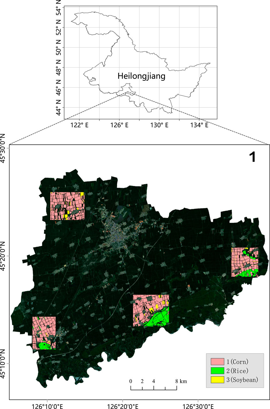
FIGURE 1. Sketch map of Sample plot in the study area.

2.2 Remote sensing satellite images

The data were obtained from GF-1 multi-spectral remote sensing image data, the first satellite in China’s Gaofen satellite series. Satellites have the advantages of combining multiple resolutions with large widths and short revisit cycles, and simultaneously realizing the combination of high resolution and large width on a single satellite, with a 2 m resolution greater than 60 km and a 16 m resolution greater than 800 km, making it one of the main data sources for agricultural remote sensing monitoring in China (Li et al., 2015). In this paper, the 2 m spatial resolution sensor carried by GF-1 satellite is used as the data source, and three scenes of multispectral remote sensing surface reflectance data with time nodes of 10/07/2020, 22/07/2020, and 26/07/2020 are selected as the test data of the model. The three scenes of data have been subjected to rapid atmospheric correction (QUAC) and geometric correction.

2.3 Ground truth

In order to obtain a larger training data set, this study adopted a practical field investigation combined with a visual interpretation method; considering the spatial distribution of crops, transportation is convenient. After the farm plot size factors, such as the design of four sample plots, the survey area involves the dual urban 12 towns and 30 villages; these sampling points of the crop planting structure are relatively stable. During the field survey, the coordinates of sample points and crop types were recorded. The visual interpretation process refers to field survey data and permanent prime farmland plot data in 2018. Quadrat data and label data were completed in ArcGIS and ENVI. The data were divided into corn, rice, soybean, and other ground object types (including buildings, roads, rivers, wetlands, etc.). Finally, 428 plot-level quadrats were obtained, and the distribution of pixel numbers and plot numbers of various types are shown in Table 1.

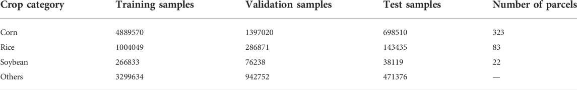
TABLE 1. Number of instances of each crop class counted at polygon- and pixel-level.

2.4 Data set

The spectral range of multi-spectral remote sensing images in the dataset is blue (0.45–0.52 μm), green (0.52–0.59 μm), red (0.63–0.69 μm) and near-infrared (0.77–0.89 μm). Two datasets were constructed using the same data source. In the first dataset, the near-infrared bands of the GF-1 remote sensing images are removed, and the remaining three bands (RGB) are normalized, which can accelerate the convergence speed of the model. The Normalized Difference Vegetation Index (NDVI) was extracted from the second dataset and combined with the first dataset to generate 4-channel samples.

In addition to using the field-measured data of tag data referring to the information of permanent basic farmland plot planting crops, in theory, the different crop plot types are relatively independent, but in practice, the condition of the same plot to sow crops, with the field-measured data, found a total of 19 major plots this phenomenon exists. ENVI and ArcGIS were used to complete the sample plot clipping, sample plot digitization, and label assignment, and four sample plots were obtained. Figure 1 shows the locations and distributions of the ground sample plots. Plots were randomly selected from four plots, and the data of the plots were divided into a training set, verification set, and test set at a ratio of 7:2:1. The data from the training set were used to train the model, the verification set was used to adjust the hyperparameters, and the test set was used to evaluate the classification results.

3 Traditional machine learning algorithms

In supervised machine learning methods, we used support vector machine (SVM) and random forest (RF) as benchmark models to compare performance with deep learning algorithms.

3.1 Support vector machine

Support vector machine (SVM), first proposed by Corinna Cortes and Vapnik (1995), is a statistical theory specifically for small samples. Its unique advantage lies in dealing with small samples, nonlinear, and high-dimensional data problems, and many scholars have applied it to remote sensing image classification tasks. It has proven superior to most other image classification algorithms in terms of classification accuracy. SVM is the maximum interval linear classifier defined in the feature space; however, it can solve the nonlinear classification problem by mapping the samples to the high-dimensional feature space. Its decision boundary is the maximum margin hyperplane solved for the learning samples (Kotsiantis et al., 2006).

For binary classification problem, suppose there are n training samples x_i, the learning target of the training samples is y_i, and the input data is T = {(x₁, y₁), (x₂, y₂),…, (x_n, y_n)}, where x_i $\in$ R_N is the input variable, and y_i $\in$ Y = {−1, 1} is the output. If there is a hyperplane for the decision boundary in the feature space of the input T (Chandra and Bedi, 2021), then

In the formula, w is the normal vector, b is the bias, and two parallel hyperplanes are constructed as the interval boundary at the decision boundary to determine the category of samples:

The positive class is above the upper interval boundary and the negative class is below the lower interval boundary.

The classification performance of SVM largely depends on the form and parameter selection of the kernel functions. Common kernel functions include linear, polynomial, radial basis function, and sigmoid functions. New kernel functions can be obtained by using a combination of kernel functions.

3.2 Random forest

The essence of the random forest algorithm is the combination of multiple decision tree classifiers (Breiman, 2001). Multiple samples are extracted from the original samples using the bootstrap resampling method. Decision tree modeling is conducted for each bootstrap sample, and then the prediction of multiple decision trees is combined to obtain the final result through voting (Wu et al., 2011). For classification problem, let the training set be T, first, the Gini index of T is calculated based on the feature. For the possible value a of feature A, test the result of A = a. according to the test result, T is divided into T₁ and T₂. The Gini index is defined as follows:

In the formula, c represents the number of categories, and p_i represents the proportion of the number of category i samples to the total number of samples. It can be seen from the formula that the smaller the Gini index, the higher the sample purity. When there is only one category of samples, the Gini index is 0. In feature a and all possible cut points a, select the feature with the smallest Gini index and its corresponding cut point as the optimal feature and cut point, split the current node into two sub nodes, divide T into two nodes according to the obtained optimal feature, recursively call the two sub nodes until the stop condition is met, and finally generate a decision tree (Liaw and Wiener, 2002).

Random forest adopts an integration algorithm with high accuracy and can maintain accuracy even if there is a large amount of missing data. Overfitting does not occur easily owing to randomly selected samples’ characteristics and some features’ random extraction in the training process (Cutler et al., 2004). Extensive studies have been conducted on the land cover classification of synthetic aperture radar (SAR) and multi-spectral remote sensing data using the random forest algorithm (Loosvelt et al., 2012; Berhane et al., 2018). Under limited real ground data, random forest exhibit excellent performance in crop classification and usually provide high classification accuracy with fast calculation speed (Nitze et al., 2012; Ustuner et al., 2019).

4 Convolutional neural network

4.1 Convolutional neural network architecture

A convolutional neural network (CNN) is a feedforward neural network constructed by imitating biological visual perception mechanisms, widely used in computer vision (LeCun et al., 2015). Since Lecun proposed the first truly meaningful convolutional neural network in 1989 (LeCun et al., 1989), the structure of a CNN is constantly changing, which is reflected in the network depth on the one hand. Some deeper networks appeared successively, such as VGG-16 and VGG-19 (Simonyan and Zisserman, 2014). However, expanding the network width enhances the convolutional function without increasing the network parameters, such as Inception (Mordvintsev et al., 2015) and Xception (Chollet, 2017). A typical convolutional neural network comprises an input, convolution, pooling, and dense layer.

4.1.1 Input layer

The input layer is the gateway to the network, and it preserves the original image structure. The original image must be pre-processed to ensure the convergence speed of the network and the training duration to map the target data to the activation function range. Common pre-processing methods include de-mean, normalization, standardization, and PCA dimensionality reduction. Augmentation of sample numbers with preset transformation rules when training samples are limited is called data augmentation, which can effectively prevent overfitting and enhance the network generalization capability. Traditional data augmentation techniques are realized by geometric transformation and color transformation of single samples and other operations. Currently, the popular variety of data strengthening techniques selects discrete samples in the training data to fit the distribution of real samples. Methods SMOTE (Chawla et al., 2002), SamplePairing (Simonyan and Zisserman, 2014) and Mixup (Inoue, 2018). Data enhancement is an implicit normalization method that does not reduce the network capacity, increasing the computational complexity, and adjusting the hyperparameter engineering quantity.

4.1.2 Convolutional layer

The convolutional layer is the core layer of the network and is used for feature extraction. It contains multiple feature maps, each composed of multiple neurons. The convolutional layer is input with several feature maps, and each neuron is locally connected to its input (Local Connectivity) (Zhang et al., 2017b). After the convolution operation, n feature graphs are output, where n is the number of convolution kernels in the convolution layer. Local connection and Weights Sharing (Waibel et al., 1989) are the main features of the convolutional layer, which can reduce the number of network parameters and increase the learning rate. Local connections represent partial connections between output neurons and input neurons on a single channel of the image, which are only used to learn local features but represent full connections in the image depth. Weights of sharing refers to when calculating the neurons of the same depth slices using convolution kernels is shared, low-level features are often generalization, have translation invariance, and the same feature may appear in different locations in the image. The same convolution kernels can be used to extract the features and train the sharing weights to reduce the network number, thus training a larger network capacity. As shown in Figure 2A is a Multi-layer Perceptron (MLP) containing three hidden layers (L₁, L₂, L₃). Owing to the use of the global sensory field, the neurons between layers are all connected, and each connection has a weight. Figure 2B is a convolutional neural network, which is composed of convolutional layers C₁, C₂ and a fully connected layer F₁. C₁ has nine neurons (x₁, x₂... x₉), C₂ has seven neurons (y₁, y₂... y₇), F₁ outputs four neurons. Due to the use of local sensory fields, each neuron in layer C₂ is only connected with part of neurons in layer C₁, rather than with all neurons, which greatly reduces the number of network parameters. At the same time, the method of sharing weights is used between C₁ layer and C₂ layer, there are only three different weights (w₁, w₂, w₃), and the weight parameters of the same set of convolutional operations are the same, and the number of parameters is further reduced, which suppresses overfitting to a certain extent.

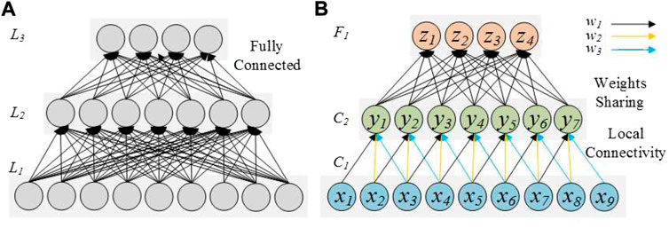
FIGURE 2. Different number of parameters generated by full connection and local connection.

The number, size, stride, and padding are hyperparameters of the convolution layer, and the convolution kernel size usually increases with an increase in the number of convolution layers (Thoma, 2017). The stride is the number of rows and columns in which the convolution kernel slides on the input image. The stride controls how the convolution kernel convolves the image and affects the extraction accuracy (Deshpande, 2017). It is necessary to add the input image to solve the problem of image edge information loss in the convolution process. Zero padding is used to fill the “0” value on the boundary of the matrix to increase the size. The relation between the input and output of the convolution layer is

Where, I_w and I_h are the width and height of the input image respectively, K_w and K_h are the width and height of the convolution kernel respectively, P is the fill, S is the stride, O is the new image generated after the convolution operation of the input image I and the convolution kernel K. Convolution is a linear operation of multiplying the input image and the convolution kernel element by element and summation, then:

Figure 3 illustrates this process.

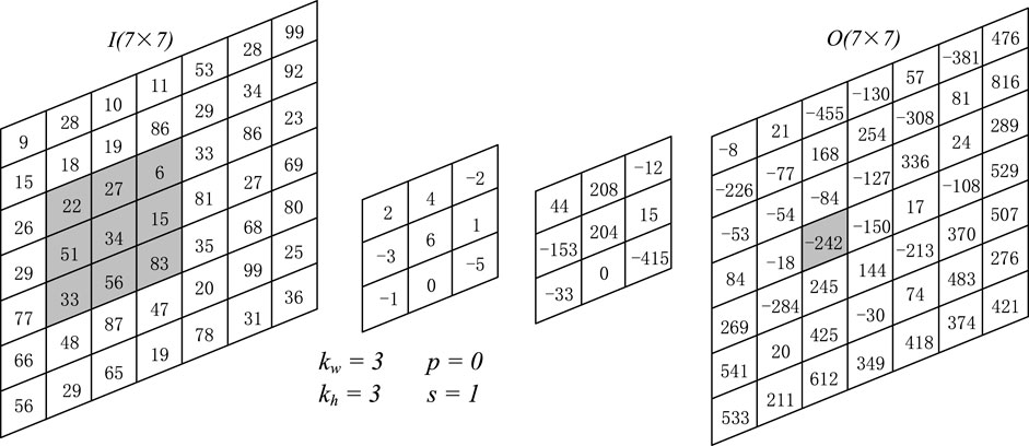
FIGURE 3. Result of Convolutional with a kernel of size 3 × 3 × 1 with stride = 1 to an image of size 7 × 7 with a single channel.

The convolutional layer extracts different input features via a convolution operation. It first extracts low-level features such as dark and bright areas and then extracts more complex features such as edges, lines, and angles. With an increase in network depth, more abstract high-level features are constructed.

4.1.3 Pooling layer

The pooling layer (the down-sampling layer) uses the convolutional layer as the input layer to continue feature extraction. Each neuron in the pooling layer is connected to some neurons in the previous layer to reduce the dimension of the input feature graph while retaining important feature information. Filter size (F) and stride (S) are the hyperparameters of pooling, where S$\in$N_>1, F = 2, and S = 2 are commonly used options, and the pooling of large receptive fields is destructive (CNNs/ConvNets, 2014).

Commonly used methods include max pooling, average pooling, spatial pyramid pooling, and stochastic pooling (Zeiler and Fergus, 2013). Maximum pooling has been proven to be the most effective method. Figure 4 shows an example of maximum pooling for a feature graph with a depth of one using a 2 × 2 filter.

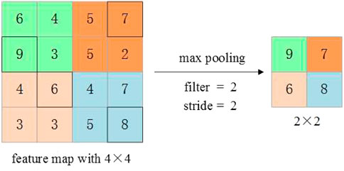
FIGURE 4. 2 × 2 max pooling applied to a feature map of size 4 × 4 with stride 2.

For the input feature graph I_w × I_h × D, where I_w is the width of the feature graph, I_h is the height of the feature graph, D is the depth, the dimension of the output feature graph is O_w × O_h × D, F is the filter, and S is the stride, then: O_w = (Iw–F)/S + 1, O_h = (I_h–F)/S + 1, it is not common to use zero fill input for maximum pooling.

The pooling layer is often inserted between continuous convolutional layers, and its function is to gradually reduce the dimensions of the input feature graph (Thoma, 2017). The pooling layer is important for the entire network.

• Reduce the number of network parameters and computations to prevent overfitting.

• The output and input feature graphs are almost the same proportion.

• Enable the network to extract certain characteristics.

• Compress features but retain some invariant features such as translation or distortion.

4.1.4 Dropout

Dropout is a regularization method that can effectively prevent network overfitting for the following reasons (Hinton et al., 2012):

• Do not change the depth or width of the network.

• In iteration, some neurons are randomly inactivated with probability p (p is usually set to 0.5), and the remaining (1—p) × m neurons are used to train the network, where m is the total number of neurons, to reduce feature redundancy.

• The random selection of neurons makes the updating of weights no longer depend on the joint action of implicit nodes with fixed relationships, which weakens the joint adaptability between neuron nodes and alleviates overfitting.

The dropout method makes the drop probability of neurons follow the Bernoulli distribution of probability p. Dropout is short for the standard dropout proposed by Hinton et al. (2010). There are many variations in the dropout methods. DropConnect, proposed by Wan et al. (2013), applies the dropout strategy to weights and biases, forcing the network to adapt to different connections during each training while giving up dropout on neurons. Ba and Frey designed another standard dropout method, Standout (Ba and Frey, 2013). The probability p of neuron inactivation is not constant but adaptive according to the weight. Wu and Gu proposed the Pooling Dropout, and directly applied the Bernoulli mask to the kernel of the largest Pooling layer before the Pooling operation. Figure 5 compares the Without Dropout, Standard Dropout and DropConnect.

FIGURE 5. When p = 0.5, the Standard Dropout activates only 50% of the neurons, and DropConnect sets 50% of the weights to zero.

4.1.5 Activation functions

The activation function is introduced to provide the network with the learning ability of nonlinear mapping to solve the nonlinear classification problem. The learning ability of a linear function is limited, and the nonlinear relationship between the input and output cannot be fully represented in the face of complex data types such as images and videos. As the convolution operation is linear, a neural network without an activation function is equivalent to a multi-layer perceptron (MLP). A neural network with an activation function can better solve the complex classification problem. Common activation functions are listed in Table 2.

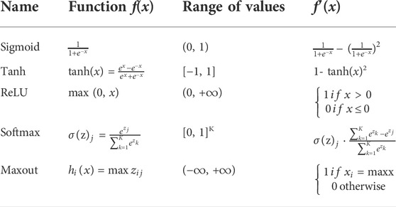
TABLE 2. Commonly used activation functions.

s(x) is the output of the sigmoid function, s(x) $\in$ (0, 1), and s(x) is symmetric, with s(x) = 0.5. It is often used in dichotomous problems and is prone to gradient explosion or gradient disappearance in deep neural networks. The tanh function is a variant of a sigmoid function. With 0 as the center, tanh(x) $\in$ [−1, 1]. Tanh also suffers from the problem of gradient disappearance. When $x\le 0$, ReLU outputs 0; when $x>0$, ReLU outputs x. ReLU can prevent gradient disappearance and accelerate network training, which is suitable for image-classification tasks. The softmax output is the discrete probability of the object being classified into different categories. The sum of all probabilities is 1, m is the number of categories, k $\in$ (0, m], i represents a certain category in k, and g_i represents the probability of this category. There are:

Maxout divides the input z into i groups and outputs the maximum value in each group. Unlike a conventional activation function, Maxout is a piecewise linear function that can be learned, and such local linearity strengthens the fitting ability of the network (Goodfellow et al., 2013). Experiments have shown that Maxout is closely related to pooling operations, and the combination of dropouts can effectively improve the network performance (Montúfar et al., 2014).

4.1.6 Dense layer

All dense layer neurons connected with all of the previous layer neurons, the connection layer integration convolution layer or pooling of category-distinct local information, will learn the convolution and pooling “distributed characteristic said” mapped to the sample tag space. The last full connection layer will be the output value passed to the softmax classifier to classify (Zhou et al., 2017). Owing to the characteristics of a full connection, the number of parameters in the full connection layer is very large. Taking AlexNet (Krizhevsky et al., 2012) as an example, the number of parameters in the three fully connected layers accounts for 96.2% of the total network parameters.

4.2 Convolutional neural networks blocks

4.2.1 Inception and xception

Unlike VGGNet, the GoogLeNet series enhances network performance by increasing the network depth. Unlike VGGNet, GoogLeNet uses Inception architecture to enhance the network width and improve the network performance by increasing the network complexity while reducing the network parameters. Inception uses convolutional kernel units of different scales to convolute or pool the input feature maps and then connects and outputs feature maps of different receptive fields. Figure 6 illustrates the topology of Inception-V3.

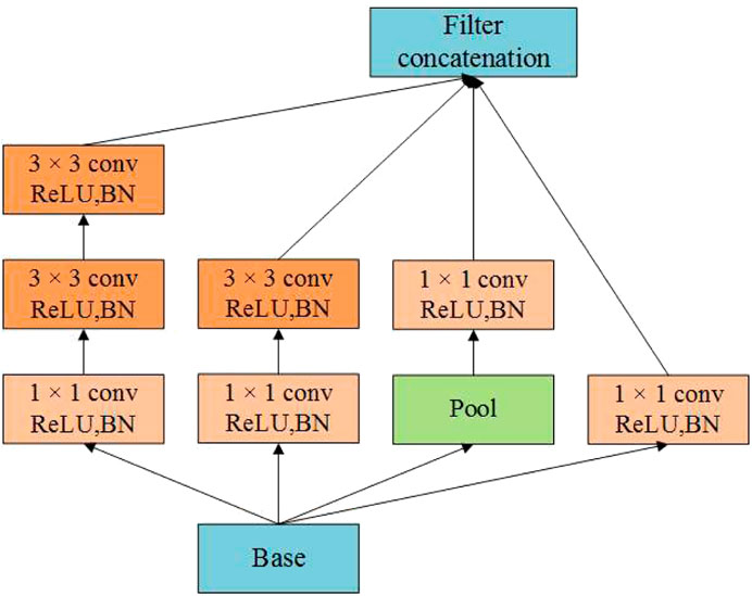
FIGURE 6. The topology of Inception-V3.

In Figure 6, all convolution units use 1 × 1 convolution kernel for dimensionality reduction, feature graphs process and reaggregate output at different scales, and the normalization method, batch normalization (BN), standardizes the output of each layer, which enables a higher learning rate and accelerates network training.

Xception improves Inception-V3 and proposes depth wise separable convolutions, whereas Inception-V3 divides the channel into four groups to perform 1 × 1 convolution computation. Xception performs a 1 × 1 convolution calculation for each channel’s feature graph and then joins the feature forces. The completely decoupled channel correlation and spatial correlation (are shown in Figure 7). Xception has the same number of parameters as Inception-V3 but performs better, and network parameters are used more efficiently (Chollet, 2017).

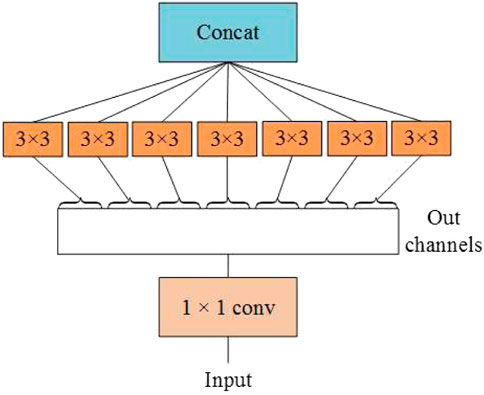
FIGURE 7. Perform the 3 × 3 convolution on each channel of the 1 × 1 convolution.

4.2.2 Residual blocks

The residual network solves the problem of network degradation with an increase in network depth. By superposing residual blocks, the accuracy of the network can be improved, even when the network depth is significantly increased. The core concept of the residual network is that a skip connection is used in the internal residual block. The information in the feature graph gradually decreases with increasing network depth, and the jump connection enables the features of the shallow layer to be transmitted to deeper layers, thus alleviating the gradient disappearance caused by the increase in depth in the shallow neural network (He et al., 2016a). The residual network provides two types of mappings, as shown in Figure 8. One is identity mapping (left part), and the other is residual mapping (right part).

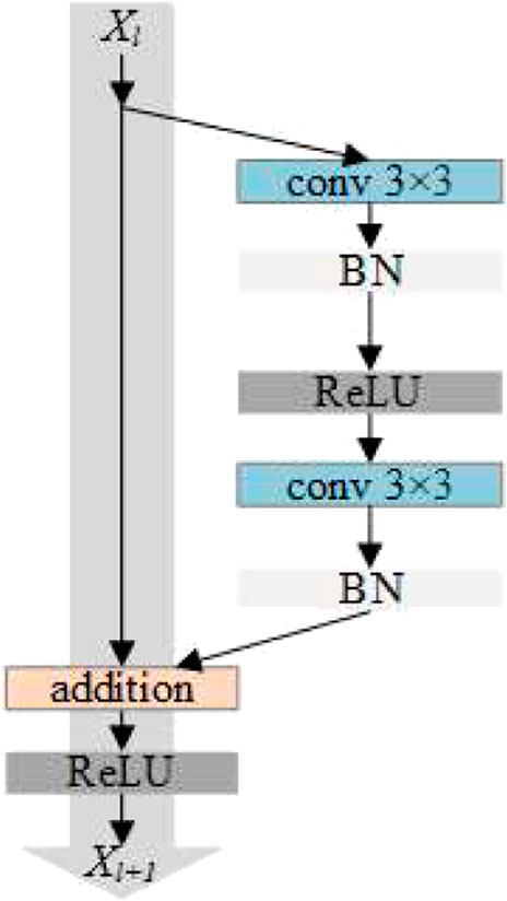
FIGURE 8. Residual block He et al. (2016b).

X_l is the input, and X_l+1 is the output, then:

The features of X_l+1 layer are composed of X_l and residual function mapping H. Deep neural networks can be constructed through residual block stacking, such as ResNet-101 and ResNet-152. In the network training process, if the optimal is achieved, H is set to 0, and only the identity mapping part is retained. Network performance did not decrease with increasing depth.

4.2.3 Dense blocks

Dense blocks are collections of convolutional layers. Within each block, all convolutional layers are directly connected, and the input of each convolutional layer is the union of the output of all previous convolutional layers, which enhances the repeated use and transmission of features to ensure maximum information flow between layers in the network. Conventional convolutional neural networks have L connections for L layer, whereas dense blocks have (L (L + 1))/2 connections (Huang et al., 2017). Dense blocks refer to the idea of Inception and Residual Blocks. In the horizontal structure, that is, within each block, the superposition of the convolution layer increases the width of the network, and the features are merged before the output. The skip connection design was used at the network depth as a reference. Feature propagation is enhanced by having each layer accept the output of all the layers before it. The Dense block is calculated as follows:

where [] represents the feature map from layers X₀ to X_L-1 combined. H_l is a nonlinear transformation implemented by Batch Normalization, activation function ReLU, and convolution calculation.

With an increase in the network depth, the dimension of the feature map increases significantly. To solve this problem, a transition layer, composed of a convolution layer and a pooling layer, is used to connect the adjacent dense blocks. The 1 × 1 convolution and 2 × 2 average pooling layers reduce the number of feature channels. Figure 9 illustrates the DenseNet with three dense blocks.

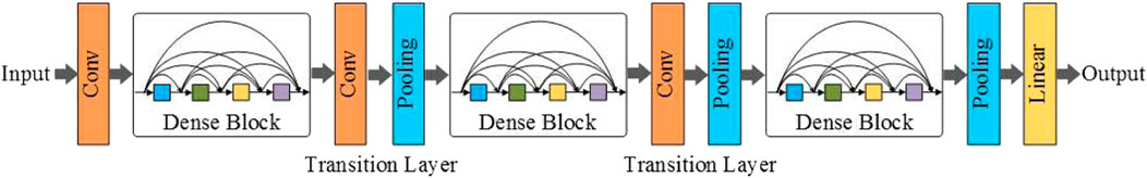
FIGURE 9. The feature map in the dense block has the same size, and the transition layer completes down-sampling.

5 Experiments

5.1 Experimental settings

The experimental design focused on the dataset, classification model selection, and model training method. First, two datasets were constructed based on the same data source to use the prior knowledge of multi-spectral remote sensing images fully. Second, on the classification model, we designed a convolutional neural network semantic segmentation model, CSNet, based on a deep learning algorithm, and compared it with the traditional machine learning algorithm.

5.1.1 Satellite data

Section 2.4 explains the differences between the two datasets used in this study. In the image classification task based on neural networks, the image data of the three channels are more common at the input layer. By modifying the input-layer structure, the network can support the data input of more channels.

The vegetation index (VI) is an important parameter for crop growth analysis and is widely used in agricultural fields. NDVI, which can measure the photosynthetic active biomass of plants, has been used by many researchers for dynamic monitoring of crop growth and crop classification (Zhang et al., 2011; Dimitrov et al., 2019; Solano-Correa et al., 2019; Zheng et al., 2021a; Zheng et al., 2021b; Li et al., 2021). Prior feature maps were constructed by adding NDVI to the RGB + NDVI datasets. The purpose was to realize a multichannel feature combination.

5.1.2 Support vector machine classifier and random forest classifier

The SVM and RF are representative non-deep-learning algorithms. For SVM and RF, we used the Python programming language and SciKit-learn (Scikit-learn, 2018) library for implementation. The hyperparameters control the model fitting. For the same dataset, each classifier has an optimal combination of hyperparameters. Experience-based tuning is suitable for a small number of hyperparameters, and when there are many hyperparameters to be tuned, this manual setting method is inefficient. Scikit-learn provides two automatic hyperparameter optimization methods, random search (RS) and grid search (GS), to improve the efficiency of hyperparameter optimization. The former uses random sampling to obtain the best combination, and the latter cross-validates all candidate hyperparameter values to reserve the combination with the highest score. Experiments have shown that RS is more efficient than GS (Bergstra and Bengio, 2012; Tian et al., 2019; Tian et al., 2020; Chen et al., 2021). For the same number of searches, RS will try more values than GS. The RS method was adopted in this study, and the hyperparameter optimization results of the SVM and RF are listed in Table 3.

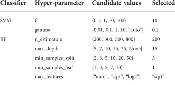
TABLE 3. The hyperparameters and candidate values of the SVM and RF classifier are optimized on both datasets using the RS method.

The SVM selects the radial basis function kernel as the kernel function, and RS selects c = 10 and gamma = 0.1 as the optimal hyperparameter combination. According to the importance of RF hyperparameters, the selection results of RS are listed in Table 3, where the number of RF spanning trees (n_estimators) is 200, and the maximum split number of each tree (max_depth) is 15. To prevent overfitting of the model due to unbalanced sample categories, the training parameter of the category weight is set to a weight that is inversely proportional to the number of sample categories so that each category has the same contribution.

The input of the above two machine learning algorithms is a comma-separated Values (CSV) file. We used Python to convert the two data sets mentioned in Section 2.4 into CSV files respectively. For RGB data sets, the CSV storage format is red band, green band, blue band and crop category labels. For RGB + NDVI dataset, the storage format in CSV is red band, green band, blue band, NDVI and crop category label.

5.1.3 Fine-tuning ResNet

With the development of deep learning technology and the support of high-performance GPU and large datasets, many convolutional neural networks with excellent architectures have been proposed. The error rate on ImageNet (Li et al., 2022) has been continuously reduced. These networks have been widely applied to various computer vision tasks with stronger feature expression abilities. The backbone refers to the shared structure of various convolutional neural network models, such as VGGNet, ResNet, and DenseNet. ResNet won the champion of image classification, image localization and image detection in the Imagenet large-scale visual recognition competition in 2015. Its proposal is considered by many scholars as a milestone event of the deep learning algorithm. The network can improve the accuracy by adding a considerable depth. The internal residual block uses jump connection, which alleviates the gradient disappearance problem caused by increasing depth in the deep neural network. It has more powerful feature extraction ability and strong universality, and is widely used in remote sensing image classification (Deng et al., 2009; Kim et al., 2014; He et al., 2016a; Cao and Zhang, 2020; Hao et al., 2020; Tian et al., 2021a; Tian et al., 2021b). In this study, we choose resnet-50 (He et al., 2016a), a deep residual network containing 50 convolutional layers, and its two variants, backbone, which we call ResNet-B (Szegedy et al., 2016) and ResNet-C (Gao et al., 2021).

Model fine-tuning and feature extraction complement each other for the new data set. Though the model fine-tuning advanced the training with custom network convergence, which is a more commonly used method, even minor adjustments may produce a significant effect on the performance of the model. In this experiment, we used the two popular ResNet adjustments. Figure 10A shows the downsampling block of the ResNet residual block. In part A of Path, the convolution kernel size is 1 × 1 with stride 2, so only a quarter of the information of the input feature graph is retained. The stride of the first convolution layer was changed to one in ResNetB to retain all the input feature graphs. The stride of the second 3 × 3 convolutional layer was changed to two, and the output shape of Path A remained unchanged in the modified structure, thus retaining more characteristic information. Figure 10B shows the structure of ResNetB. ResNetC changes Path B of resNET-50’s downsampling block and replaces the original convolutional layer with a convolution kernel size of 1 × 1, stride 2 into an average pooling layer with a pooling size of 2, stride of 2, and a convolution kernel size of 1 × 1. For the convolution layer with stride 2, this modification retains all the input feature maps, as shown in Figure 10C.

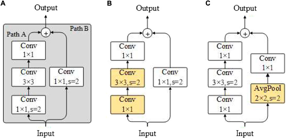
FIGURE 10. The architecture of ResNet-50 and ResNetB and ResNetC. (A) ResNet-50 (B) ResNetB (C) ResNetC.

In this study, we designed a convolutional neural network CSNet based on an encoder-decoder architecture for the semantic segmentation of crops. The encoder used the three residual networks listed in Figure 10 as the backbone to extract features. In the decoder part, deconvolution and upsampling are used to recover the spatial information lost in the encoder gradually. Finally, Softmax outputs the probability values of the different categories for each pixel. The network architecture is shown in Figure 11.

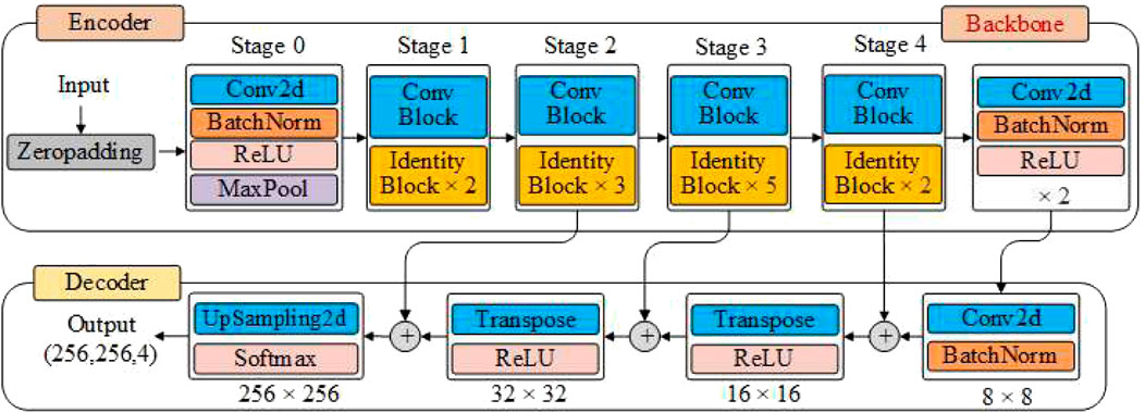
FIGURE 11. Architecture of the CSNet model.

Before deep learning model training, the two datasets mentioned in Section 2.4 were preprocessed respectively. We randomly cropped 256 × 256 images from four sample plots in the dataset as the input of the model, the resolution of the input image is 256 × 256. The images cropped from the two datasets have the same resolution, but the number of channels is different. This is done in the Python language through the OpenCV library.

In the encoder part, for the RGB data set, each image has three channels, and the shape of the input is (256, 256, 3); for the dataset with the NDVI feature, each image has four channels, and the shape of the input is (256, 256, 4). We deleted the global average pooling layer and dense layer from the backbone. After Stage 4, a convolution layer with a 3 × 3 convolution kernel size and stride of one was added. Then, a BN layer was then added with ReLU as the activation function. In this case, the number of feature graph outputs from the model was the same as that from Stage 4. The output shape is (8, 8, 2048). In the decoder part, we added a convolutional layer and a BN layer to obtain the same number of output channels as the number of crop categories in the mission, with output shapes of (8, 8, 4). Then, upsampling was performed using two deconvolution units. In the first deconvolution unit, the number of channels output by Stage 3 is the same as the number of crop categories by adding a deconvolution layer and a BN layer. Deconvolution with a 3 × 3 convolution kernel size and stride 2 was used to up-sample the input to (16, 16, 4). Finally, the deconvolution output is added to the output of Stage 3, and the result is inputted to the next deconvolution unit. In the second deconvolution unit, the calculation process was the same as the first deconvolution unit, except that Stage 3 was replaced by Stage 2, and the output shape was (32, 32, 4). At the end of the model, the up-sampling layer and activation function softmax were used to up-sample the output results of the second deconvolution unit eight times and restore the image to the input size of 256 × 256. The output shape was (256, 256, 4), where four is the probability that each pixel is divided into four categories.

We used the Keras deep learning framework and TensorFlow as the backend to realize CSNet. The CSNet of different backbones uses the same hyperparameters in the two datasets to conduct experiments. The optimizer uses the adaptive learning rate algorithm Adam (Kingma and Ba, 2014). The initial learning rate was set to 1 × 10⁻⁴, and the learning rate was attenuated to 1 × 10⁻⁵. The loss function adopts the widely used categorical cross-entropy, and the batch size was set to 15. The model was trained for 200 epochs on each dataset. Early stopping is a method used to avoid network overfitting. When the performance of the model on the verification set does not increase, training can be stopped in advance. In the experiment, model training was stopped when the maximum accuracy was not reached in 30 consecutive epochs, and the model with the best performance was saved on the test set. Figure 12 shows the training process for obtaining the highest classification accuracy on the two datasets for the three different backbone CSNet models. With an increase in the number of iterations, the model converges rapidly, the classification accuracy gradually improves, and no fitting occurs. Owing to the use of early stopping, CSNet (resnet-50) and CSNet (ResNetB) stopped training after iterating 140 epochs and 160 epochs on the RGB dataset. Simultaneously, we applied the data enhancement strategy of the Keras framework to expand the samples randomly in the input layer of the model. During model training, we noticed that the errors in the validation set could be significantly reduced by using data augmentation, with the total training duration of the model being up to 800 h. The operating environment used an Intel Xeon E5-1650 V4 processor, an NVIDIA Quadro P4000 GPU, and 64 GB of memory.

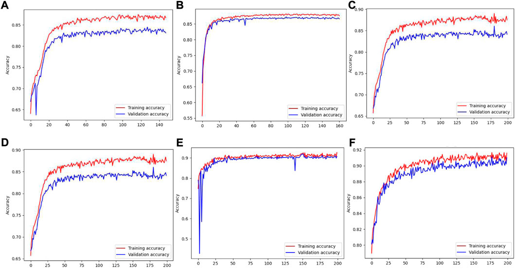
FIGURE 12. (A–C) The training process of CSNet (ResNet-50), CSNet (ResNetB), CSNet (ResNetC) on RGB dataset. (D–F) The training process of CSNet (ResNet-50), CSNet (ResNetB), CSNet (ResNetC) on RGB + NDVI dataset.

The overall accuracy (OA), kappa average coefficient, and mean intersection over union (MIoU) were used as the evaluation indicators to evaluate the performance of all classifiers.

5.2 Results

GF-1 data processed in Section 2.4 were taken as input. The machine learning algorithm (RF and SVM) in Section 3 and the CSNet model proposed in this paper were used for classification, and each classifier was cross-verified five times. The test results and indicators for the two datasets are listed in Table 4.

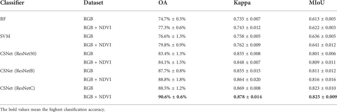
TABLE 4. Over accuracy, kappa averaged (±one standard deviation) and MIoU for every classifier.

The classification results show that, for the same classifier, the average classification accuracy of the RGB + NDVI dataset is slightly better, indicating that adding NDVI features helps improve the classification accuracy. For different classifiers, the performance of SVM was slightly better than that of RF, and the performance of the three classifiers based on the deep learning algorithm was better than that of the machine learning algorithm. CSNet, which uses ResNetC as the backbone, achieves the highest classification accuracy in the RGB + NDVI dataset. The results were 13.3 and 9.5 percentage points higher than those of RF and SVM and 5.6 and 0.6 percentage points higher than those of CSNet (ResNet-50) and CSNet (ResNetB), respectively.

Figure 13 shows that the classification results of RF and SVM on the two data sets are discontinuous, with unclear boundaries, obvious misclassification of corn and background, and a big gap between the precision and the classification results of a deep learning algorithm. In model training, RF and SVM can quickly fit sample data, but the prediction efficiency is low. The deep learning model takes a long time to train, and the average training time of the model used in this paper is about 40 h. Semantic segmentation is pixel-level classification, which can predict the whole image, making it more efficient. Thanks to the powerful feature extraction capability of the residual network, CSNet of three different Backbone has achieved good classification effect and high classification accuracy on two data sets. With a clear plot boundary, few noise points and relatively few error classification areas, it has achieved the highest classification accuracy of 89.7% on RGB data sets. In the RGB + NDVI data set, CSNet (ResNetC) achieved the highest classification accuracy of 91.2%, and OA, Kappa and MIoU indexes were the highest. By comparing (c) and (h), (d) and (I), it can be found that, for RF and SVM, relatively few backgrounds in RGB + NDVI data sets are misclassified into crop categories, which is caused by the enhanced sensitivity of NDVI to low vegetation density coverage areas. This phenomenon also exists in CSNet, but it is not obvious. The classification results of CSNet (ResNetC) on the RGB + NDVI data set are shown in Figure 14, see Figure 13 for legend. There is no obvious stitching trace in the crop distribution map, and the spatial distribution of corn, rice and soybean, as well as the background of buildings and roads, can be identified visually.

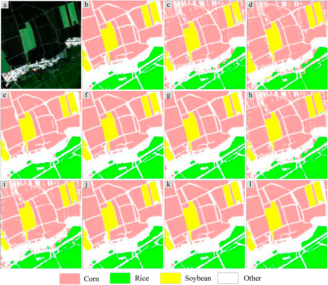
FIGURE 13. Comparison between machine learning algorithm and deep learning algorithm for image classification. (A) The original data. (B) Ground truth. (C–G) Results of RF, SVM, ResNet50, ResNetB, ResNetC based on RGB dataset, (H–L) Results of RF, SVM, ResNet50, ResNetB, ResNetC based on RGB + NDVI dataset.

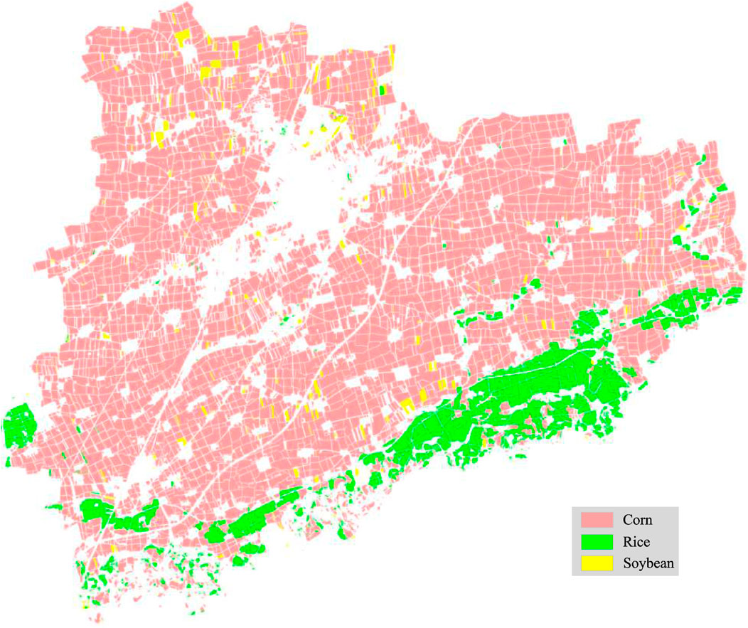
FIGURE 14. The classification result of CSNet (ResNetC).

5.3 Discussion

The research in this study shows that high-resolution remote sensing data are suitable for crop classification, and the introduction of NDVI as an auxiliary feature variable can improve classification accuracy. Based on a comparative analysis of traditional machine learning algorithms such as RF and SVM, we built CSNet, a semantic segmentation network that can identify crops at the plot scale. Both the traditional machine learning and advanced deep learning algorithms achieved good classification results on the two datasets. The overall accuracy of the deep learning algorithm was greater than 80%, and the kappa coefficient was greater than 0.8. The experimental results show that the CSNet model is suitable for crop mapping and estimating crop planting area and is an effective supplementary method for crop surveys.

The model of classification performance is largely dependent on the amount and type of training samples (Wang et al., 2019), the main crops are corn, rice, and soybeans, among which the former two crops planting area of more than 90% of the total sown area; the planting structure of soybean field sampling work has brought the difficulty, also led to the sample not being balanced, making the model easy to fit, and problems with poor generalization ability. Therefore, we used the following two methods to solve the sample imbalance problem: During model training, a data enhancement strategy was used in the model input layer to expand the categories with fewer samples. Simultaneously, the sampling strategy is modified to increase the selection probability of categories with fewer samples. We also found crops such as wheat and Chinese medicinal materials during the field sampling process. According to the years of statistical data, the sown area of these crops is less than 1% of the total sown area. Therefore, these crops are classified as background, which is also one of the reasons for the large background areas in the middle of the individual plots.

With the development of sensor technology, satellite data sources with high resolution and high temporal and spatial resolution in agricultural areas are becoming increasingly abundant, increasing the ability to obtain remote sensing satellite data in large agricultural areas. In deep learning, when the conditions of the application scenario are similar, one can learn by migration (Pan and Qiang, 2010), the parameter and the knowledge migration, using the training model to support the new task in this trial. We also tried applying the CSNet model to study areas near other agricultural regions and achieved a higher classification accuracy, especially when remote sensing satellite data are similar in time.

6 Conclusion

In this study, GF-1 images were used as data sources to construct two datasets of crops in agricultural areas: RGB and RGB + NDVI. Traditional machine learning algorithms and deep learning algorithms were compared and analyzed. CSNet, a semantic segmentation network for crop classification, was proposed to realize fine crop remote-sensing classification. The main conclusion are as follows.

1) The overall classification accuracy and classification effect of the deep learning algorithm were better than those of the machine-learning algorithm. Fine-tuning can affect the feature extraction ability of the backbone network, thus affecting the model performance. According to the accuracy evaluation results, the CSNet of the backbone network using ResNetC with fine-tuning has the highest classification accuracy. It can reach 91.2%. In terms of the classification effect, the classification results of the deep-learning algorithm were more precise.

2) Compared with the classification accuracy of all classifiers on the two data sets, it can be seen that the addition of NDVI features helps improve the classification accuracy of crops, especially for machine learning algorithms, but the model performance improvement is limited for deep learning algorithms.

3) The system constructed in this study can effectively improve the classification accuracy of crops, and the pre-training model can be applied to a wider range of crop recognition tasks in agricultural areas through transfer learning, providing a reference for the real-time acquisition of crop planting structure information in agricultural areas.

Data availability statement

The original contributions presented in the study are included in the article/supplementary material, further inquiries can be directed to the corresponding author.

Author contributions

TL contributed to conception and design of the study. LuW organized the database. LeW performed the statistical analysis. TL wrote the first draft of the manuscript. All authors contributed to manuscript revision, read, and approved the submitted version.

Conflict of interest

The authors declare that the research was conducted in the absence of any commercial or financial relationships that could be construed as a potential conflict of interest.

Publisher’s note

All claims expressed in this article are solely those of the authors and do not necessarily represent those of their affiliated organizations, or those of the publisher, the editors and the reviewers. Any product that may be evaluated in this article, or claim that may be made by its manufacturer, is not guaranteed or endorsed by the publisher.

References

Ba, J., and Frey, B. (2013). “Adaptive dropout for training deep neural networks,” in Advances in neural information processing systems, 3084–3092.
Belenguer-Plomer, M. A., Tanase, M. A., Chuvieco, E., and Bovolo, F. (2021). CNN-based burned area mapping using radar and optical data. Remote Sens. Environ. 260, 112468. doi:10.1016/j.rse.2021.112468
Bergstra, J., and Bengio, Y. (2012). Random search for hyper-parameter optimization. J. Mach. Learn. Res. 13 (1), 281–305. doi:10.1016/j.chemolab.2011.12.002
Berhane, T. M., Lane, C. R., Wu, Q. S., Autrey, B. C., Anenkhonov, O. A., Chepinoga, V. V., et al. (2018). Decision-tree, rule-based, and random forest classification of high-resolution multispectral imagery for wetland mapping and inventory. Remote Sens. 10 (4), 580. doi:10.3390/rs10040580
Cao, K., and Zhang, X. (2020). An improved Res-UNet model for tree species classification using airborne high-resolution images. Remote Sens. 12 (7), 1128. doi:10.3390/rs12071128
Chandra, M. A., and Bedi, S. S. (2021). Survey on SVM and their application in image classification. Int. J. Inf. Technol. 13 (5), 1–11. doi:10.1007/s41870-017-0080-1
Chawla, N. V., Bowyer, K. W., Hall, L. O., and kegelmeeyere, W. P. (2002). Smote: Synthetic minority over-sampling technique. J. Artif. Intell. Res. 16 (1), 321–357. doi:10.1613/jair.953
Chen, J., Du, L., and Guo, Y. (2021). Label constrained convolutional factor analysis for classification with limited training samples. Inf. Sci. 44, 372–394. doi:10.1016/j.ins.2020.08.048
Chollet, F. (2017). “Xception: Deep learning with depthwise separable convolutions,” in Proceeding of the 2017 IEEE Conference on Computer Vision and Pattern Recognition (CVPR), Honolulu, HI, USA, July 2017 (IEEE), 1800–1807.
CNNs/ConvNets (2014) Convolutional neural networks (CNNs/ConvNets). Available at: https://cs231n.github.io/convolutional-networks/.
Conrad, C., Dech, S., Dubovyk, O., Fritsch, S., Klein, D., Löw, F., et al. (2014). Derivation of temporal windows for accurate crop discrimination in heterogeneous croplands of Uzbekistan using multitemporal RapidEye images. Comput. Electron. Agric. 103, 63–74. doi:10.1016/j.compag.2014.02.003
Deng, J., Dong, W., Socher, R., Li, L. J., Li, K., and Li, F. (2009). “ImageNet: A large-scale hierarchical image database,” in Proceeding of the 2009 IEEE Conference on Computer Vision and Pattern Recognition, Miami, FL, USA, June 2009 (IEEE), 248–255.
Deshpande, A. (2017). A beginner’s guide to understanding convolutional neural networks. Adeshpande3.github.io. Available at: https://adeshpande3.github.io/adeshpande3.github.io/A-Beginner’s-Guide-To Understanding-Convolutional-Neural-Networks/ (Accessed 08Apr, 2017).
Dimitrov, P., Dong, Q. H., Eerens, H., Gikov, A., Filchev, L., Roumenina, E., et al. (2019). Sub-pixel crop type classification using PROBA-V 100 m NDVI time series and reference data from sentinel-2 classifications. Remote Sens. 11 (11), 1370. doi:10.3390/rs11111370
Feng, Q. L., Niu, B. W., Zhu, D. H., Liu, Y. M., Ou, C., and Liu, J. T. (2022). Classification of farmland plastic cover based on multi-core active learning and multi-source data fusion. Trans. Chin. Soc. Agric. Mach. 53 (2), 177–185. doi:10.6041/j.issn.1000-1298.2022.02.018
Gao, S. H., Cheng, M. M., Zhao, K., Zhang, X. Y., Yang, M. H., and Torr, P. (2021). Res2Net: A new multi-scale backbone architecture. IEEE Trans. Pattern Anal. Mach. Intell. 43 (2), 652–662. doi:10.1109/tpami.2019.2938758
Goodfellow, I., Warde-Farley, D., Mirza, M., Courville, A., and Bengio, Y. (2013). “Maxout networks,” in Proceedings of the 30th international conference on machine learning, 1319–1327.
Hao, S., Wang, W., and Salzmann, M. (2020). Geometry-aware deep recurrent neural networks for hyperspectral image classification. IEEE Trans. Geosci. Remote Sens. 59 (3), 2448–2460. doi:10.1109/tgrs.2020.3005623
Hasegawa, T., Sakurai, G., Fujimori, S., Takahashi, K., Hijioka, Y., and Masui, T. (2021). Extreme climate events increase risk of global food insecurity and adaptation needs. Nat. Food 2, 587–595. doi:10.1038/s43016-021-00335-4
He, K., Zhang, X., Ren, S., and Sun, J. (2016). “Deep residual learning for image recognition,” in Proceeding of the 2016 IEEE Conference on Computer Vision and Pattern Recognition (CVPR), June 2016, 770–778.
He, K. M., Zhang, X. Y., Ren, S. Q., and Sun, J. (2016). “Identity mappings in deep residual networks,” in European conference on computer vision (Cham: Springer), 630–645.
Hinton, G. E., Srivastava, N., Krizhevsky, A., Sutskever, I., and Salakhutdinov, R. R. (2012). Improving neural networks by preventing co-adaptation of feature detectors. Comput. Sci. 3 (4), 212–223. doi:10.48550/arXiv.1207.0580
Hu, Q., Wu, W. B., Song, Q., Yu, Q. Y., Yang, P., and Tang, H. J. (2015). Recent progresses in research of crop patterns mapping by using remote sensing. Sci. Agric. Sin. 48 (10), 1900–1914. doi:10.3864/j.issn.0578-1752.2015.10.004
Huang, G., Liu, Z., Laurens, V. D., and Weinberger, K. Q. (2017). “Densely connected convolutional networks,” in Proceeding of the 2017 IEEE Conference on Computer Vision and Pattern Recognition (CVPR), Honolulu, HI, USA, July 2017 (IEEE), 2261–2269.
Inoue, H. Data augmentation by pairing samples for images classification. 2018, doi:10.48550/arXiv.1801.02929
Jiang, T., and Wang, X. J. (2019). Commentary on: Finite element analysis of the effect of sagittal angle on ankle joint stability in posterior malleolus fracture: A cohort study. Int. J. Surg. 41 (9), 20–29. doi:10.1016/j.ijsu.2019.09.008
Jin, Z., Azzari, G., and Lobell, D. B. (2017). Improving the accuracy of satellite-based high-resolution yield estimation: A test of multiple scalable approaches. Agric. For. Meteorology 247, 207–220. doi:10.1016/j.agrformet.2017.08.001
Kim, Y., Kimball, J. S., Zhang, K., Didan, K., Velicogna, I., and McDonald, K. C. (2014). Attribution of divergent northern vegetation growth responses to lengthening non-frozen seasons using satellite optical-NIR and microwave remote sensing. Int. J. Remote Sens. 35 (10), 3700–3721. doi:10.1080/01431161.2014.915595
Kingma, D. P., and Ba, J. (2014). Adam: A method for stochastic optimization. doi:10.48550/arXiv.1412.6980
Kotsiantis, S. B., Zaharakis, I. D., and Pintelas, P. E. (2006). Machine learning: A review of classification and combining techniques. Artif. Intell. Rev. 26, 159–190. doi:10.1007/s10462-007-9052-3
Krizhevsky, A., Sutskever, I., and Hinton, G. E. (2012). “Imagenet classification with deep convolutional neural networks,” in Advances in neural information processing systems 25 (NIPS). F. Pereira, C. J. C. Burgeset al. (Curran Associates, Inc.), 1097–1105.
Kussul, N., Lavreniuk, M., Skakun, S., and Shelestov, A. (2017). Deep learning classification of land cover and crop types using remote sensing data. IEEE Geosci. Remote Sens. Lett. 14 (5), 778–782. doi:10.1109/lgrs.2017.2681128
LeCun, Y., Bengio, Y., and Hinton, G. (2015). Deep learning. Nature 521 (7553), 436–444. doi:10.1038/nature14539
LeCun, Y., Boser, B., Denker, J. S., Henderson, D., Howard, R. E., Hubbard, W., et al. (1989). Backpropagation applied to handwritten zip code recognition. Neural Comput. 1 (4), 541–551. doi:10.1162/neco.1989.1.4.541
Li, F., Wang, L., Liu, J., and Chang, Q. (2015). Remote sensing estimation of SPAD value for wheat leaf based on GF-1 data. Trans. Chin. Soc. Agric. Mach. 46, 273–281. doi:10.6041/j.issn.1000-1298.2015.09.040
Li, S., Liu, C. H., Lin, Q. X., Wen, Q., Su, L. M., Huang, G., et al. (2021). Deep residual correction network for partial domain adaptation. IEEE Trans. Pattern Anal. Mach. Intell. 43 (7), 2329–2344. doi:10.1109/tpami.2020.2964173
Li, Y., Du, L., and Wei, D. (2022). Multiscale CNN based on component analysis for SAR ATR. IEEE Trans. Geosci. Remote Sens. 60, 1–12. doi:10.1109/tgrs.2021.3100137
Liaw, A., and Wiener, M. (2002). Classification and regression by random forest. R. News 2/3, 18–22.
Loosvelt, L., Peters, J., Skriver, H., de Baets, B., and Verhoest, N. E. (2012). Impact of reducing polarimetric sar input on the uncertainty of crop classifications based on the random forests algorithm. IEEE Trans. Geosci. Remote Sens. 50 (10), 4185–4200. doi:10.1109/tgrs.2012.2189012
Maggiori, E., Tarabalka, Y., Charpiat, G., and Alliez, P. (2017). Convolutional neural networks for large-scale remote sensing image classification. IEEE Trans. Geosci. Remote Sens. 55 (2), 645–657. doi:10.1109/tgrs.2016.2612821
Marmanis, D., Schindler, K., Wegner, J. D., Galliani, S., Datcu, M., and Stilla, U. (2018). Classification with an edge: Improving semantic image segmentation with boundary detection. ISPRS J. Photogramm. Remote Sens. 135, 158–172. doi:10.1016/j.isprsjprs.2017.11.009
Ming, D. P., Luo, J. C., Shen, Z. F., Wang, M. M., and Sehng, H. (2005). Research on information extraction and target recognition from high resolution remote sensing images. Sci. Surv. Mapp. 30 (3), 18–21. doi:10.3771/j.issn.1009-2307.2005.03.004
Montúfar, G., Pascanu, R., Cho, K., and Bengio, Y. (2014). “On the number of linear regions of deep neural networks,” in NIPS’14: Proceedings of the 27th International Conference on Neural Information Processing Systems, December 2014, 2924–2932. vol. 2.
Mordvintsev, A., Olah, C., and Tyka, M. (2015). Inceptionism: Going deeper into neural networks. Corpus ID: 69951972.
Nitze, I., Schulthess, U., and Asche, H. (2012). “Comparison of machine learning algorithms random forest, artificial neural network and support vector machine to maximum likelihood for supervised crop type classification,” in Proceedings of the 4th GEOBIA, Rio de Janeiro, Brazil, 7–9 May 2012, 35.
Pan, S. J., and Qiang, Y. (2010). A survey on transfer learning. IEEE Trans. Knowl. Data Eng. 22 (10), 1345–1359. doi:10.1109/tkde.2009.191
Rustowicz, R. M., Cheong, R., Wang, L., Ermon, S., Burke, M., and Lobell, D. B. (2019). “Semantic segmentation of crop type in Africa: A novel dataset and analysis of deep learning methods,” in Comput. Vis. Pattern Recognit, 75–82.
Scikit-learn (2018). WWW4 scikit-learn: Machine learning in Python. Available at: http://scikit-learn.org/ (Accessed date: October 22, 2018).
Simonyan, K., and Zisserman, A. Very deep convolutional networks for large-scale image recognition. 2014, doi:10.48550/arXiv.1409.1556
Solano-Correa, Y. T., Bovolo, F., and Bruzzone, L. (2019). “A semi-supervised crop-type classification based on sentinel-2 NDVI satellite image time series and phenological parameters,” in Proceedings of the IGARSS 2019 - 2019 IEEE International Geoscience and Remote Sensing Symposium, Yokohama, Japan, July 2019 (IEEE), 457–460.
Suykens, J. A. K., and Vandewalle, J. (1999). Least squares support vector machine classifiers. Neural Process. Lett. 9, 293–300. doi:10.1023/a:1018628609742
Szegedy, C., Vanhoucke, V., Ioffe, S., Shlens, J., and Wojna, Z. (2016). “Rethinking the inception architecture for computer vision,” in CVPR, June 2016 (IEEE), 2818–2826.
Thoma, M. Analysis and optimization of convolutional neural network architectures. 2017, doi:10.48550/arXiv.1707.09725
Tian, H., Huang, N., Niu, Z., Qin, Y., Pei, J., and Wang, J. (2019). Mapping winter crops in China with multi-source satellite imagery and phenology-based algorithm. Remote Sens. (Basel, Switz. 11 (7), 820. doi:10.3390/rs11070820
Tian, H., Pei, J., Huang, J., Li, X., Wang, J., Zhou, B., et al. (2020). Garlic and winter wheat identification based on active and passive satellite imagery and the Google Earth engine in northern China. Remote Sens. 12 (3539), 3539. doi:10.3390/rs12213539
Tian, H., Qin, Y., Niu, Z., Wang, L., and Ge, S. (2021). Summer maize mapping by compositing time series sentinel-1A imagery based on crop growth cycles. J. Indian Soc. Remote Sens. 49 (11), 2863–2874. doi:10.1007/s12524-021-01428-0
Tian, H., Wang, Y., Chen, T., Zhang, L., and Qin, Y. (2021). Early-season mapping of winter crops using sentinel-2 optical imagery. Remote Sens. 13 (19), 3822. doi:10.3390/rs13193822
Ünsalan, C., and Boyer, K. L. (2011). Multispectral satellite image understanding. London: Springer.
Ustuner, M., Sanli, F. B., Abdikan, S., Bilgin, G., and Goksel, C. (2019) “A booster analysis of extreme gradient boosting for crop classification using PolSAR imagery,” in Proceedings of the 2019 8th International Conference on Agro-Geoinformatics (Agro-Geoinformatics), Istanbul, Turkey, 16–19 July 2019 (IEEE), 1–4.
Waibel, A., Hanazawa, T., Hinton, G., Shikano, K., and Lang, K. J. (1989). Phoneme recognition using time-delay neural networks. IEEE Trans. Acoust. 37 (3), 328–339. doi:10.1109/29.21701
Wan, L., Zeiler, M., Zhang, S., LeCun, Y., and Fergus, R. (2013). Regularization of neural networks using dropconnect. J. Mach. Learn. Res. 28, 1058–1066.
Wang, M., Chen, J. Y., Wang, G., Gao, F., Sun, K., and Xu, M. Z. (2019). Remote sensing image object sample generation method for deep learning. Foreign Electron. Meas. Technol. 38 (4), 60–65. doi:10.19652/j.cnki.femt.1801269
Wang, L., Buitenwerf, R., Munk, M., Bøcher, P. K., and Svenning, J. C. (2020). Deep-learning based high-resolution mapping shows woody vegetation densification in greater Maasai Mara ecosystem. Remote Sens. Environ. 247, 111953. doi:10.1016/j.rse.2020.111953
Wei, S., Zhang, H., Wang, C., Wu, F., and Zhang, B. (2019). “Corn fine classification with GF-3 high-resolution sar data based on deep learning,” in Proceedings of the IGARSS 2019 - 2019 IEEE International Geoscience and Remote Sensing Symposium, Yokohama, Japan, July 2019 (IEEE), 6397–6400.
Wu, J. B., Zhu, J. P., and Xie, B. C. (2011). A review of technologies on random forests. J. Statistics Inf. 26 (3), 32–38. doi:10.3969/j.issn.1007-3116.2011.03.006
Xia, T., Wu, W. B., Qingbo Zhou, Q. B., Zhou, Y., Luo, J., Yang, P., et al. (2016). Spatialization of statistical crop planting area based on geographical regression. J. Nat. Resour. 31 (30), 1773–1782. doi:10.11849/zrzyxb.20151259
Yang, S. T., Gu, L. J., Li, X. F., Jiang, T., and Ren, R. Z. (2020). Crop classification method based on optimal feature selection and hybrid CNN-RF networks for multi-temporal remote sensing imagery. Remote Sens. 12 (19), 3119. doi:10.3390/rs12193119
Zeiler, M. D., and Fergus, R. Stochastic pooling for regularization of deep convolutional neural networks. 2013, doi:10.48550/arXiv.1301.3557
Zhang, S. W., Lei, Y. P., Wang, L. P., Li, H. J., and Zhao, H. B. (2011). Crop classification using modis NDVI data denoised by wavelet: A case study in hebei plain, China. Chin. Geogr. Sci. 21, 322–333. doi:10.1007/s11769-011-0472-2
Zhang, W., Zheng, K., Tang, P., and Zhao, L. J. (2017). Deep convolutional neural network feature extraction for land cover classification. J. Image Graph. 22 (8), 1144–1153. doi:10.11834/jig.170139
Zhang, H., Cisse, M., Dauphin, Y. N., and Lopez-Paz, D. Mixup: Beyond empirical risk minimization. 2017. doi:10.48550/arXiv.1710.09412
Zheng, W., Liu, X., Ni, X., Yin, L., and Yang, B. (2021). Improving visual reasoning through semantic representation. IEEE Access 9, 91476–91486. doi:10.1109/access.2021.3074937
Zheng, W., Liu, X., and Yin, L. (2021). Sentence representation method based on multi-layer semantic network. Appl. Sci. 11 (3), 1316. doi:10.3390/app11031316
Keywords: crop classification, high resolution remote sensing, deep learning, convolutional neural network, semantic segmentation
Citation: Lu T, Wan L and Wang L (2022) Fine crop classification in high resolution remote sensing based on deep learning. Front. Environ. Sci. 10:991173. doi: 10.3389/fenvs.2022.991173
Received: 11 July 2022; Accepted: 20 September 2022;
Published: 06 October 2022.
Edited by:
Ana Maria Tarquis, Polytechnic University of Madrid, SpainReviewed by:
Oumayma Bounouh, National School of Computer Sciences, La Manouba, TunisiaJavier Borondo, Comillas Pontifical University, Spain
Copyright © 2022 Lu, Wan and Wang. This is an open-access article distributed under the terms of the Creative Commons Attribution License (CC BY). The use, distribution or reproduction in other forums is permitted, provided the original author(s) and the copyright owner(s) are credited and that the original publication in this journal is cited, in accordance with accepted academic practice. No use, distribution or reproduction is permitted which does not comply with these terms.
*Correspondence: Luhe Wan, wanluhe@sina.com