Evaluation of coupled model intercomparison project phase 6 models in simulating precipitation and its possible relationship with sea surface temperature over Myanmar

1 Introduction

In many modelling studies, global warming has been linked to extreme events. These extreme events have intensified across many regions around the globe (IPCC 2021) and led to several natural disasters that have resulted in losses of lives and property (Amato et al., 2019; Iqbal et al., 2019; IPCC 2021). One such region is Myanmar, where the spatiotemporal variability of the changes in precipitation means that understanding the performance of models in simulating precipitation over this country is an important line of research (Kitoh et al., 2013). Myanmar is a country in Southeast Asia that experiences harsh consequences of climate change, mainly in the form of flooding and drought over whole or part of the country.

To study historical extreme events, observational data and global climate model (GCM) outputs are used (Taylor et al., 2012; O’Neill et al., 2016). The Coupled Model Intercomparison Project (CMIP) is a project framework that compares GCMs in an attempt to help further our understanding of the reaction of the climate system to different scenarios of anthropogenic warming. The ability of climate models to simulate precipitation variations in the globe and some regions that showed obvious warming and wetting trends result from different levels of anthropogenic warming (Taylor et al., 2012; Meehl et al., 2014; Eyring et al., 2016; O'Neill et al., 2016), with past studies having revealed these findings on the basis of the Coupled Model Intercomparison Project Phase 5 (CMIP5) and older versions (Babar et al., 2014; Alexander 2016; Ge et al., 2019; Ge et al., 2021). Despite these findings from global and regional climate models, there is no consensus on the historical change in precipitation. Several reasons have been proposed for this lack of consensus, but data quality and limitations to the coverage of data are viewed as the major obstacles (Alexander 2016).

Additionally, there were reports that argued the limitations in CMIP data are due to their respective configurations, CMIP5 models and their older versions find it difficult to detect historical trends at time scales long enough to overcome the natural variability of the climate. However, in the latest release of CMIP namely the CMIP6, new radiative forcings used by authors and the improved quality and resolution of the models provide a better representation of the responses of the climate system, which is of great interest for vulnerability impact assessment studies (Stoufferet al., 2017). In addition, specific to the present study, this is particularly important in addressing the variability of precipitation in different climate regions. For instance, the skill of CMIP6 GCMs in simulating the variability of precipitation over Asia has been demonstrated (Wang et al., 2018; Fremme and Sodemann 2019).

Several studies on evaluating CMIP6 GCMs over Asia have been conducted (Jiang et al., 2007; Jiang et al., 2012; Dong et al., 2018; He and Zhao, 2018; Iqbal et al., 2021). For example, Iqbal et al. (2021) found that CMIP6 models reproduce the spatial patterns of precipitation well over mainland Southeast Asia. However, a study that considers as large a region as this may with the same approach fail to depict the features of a relatively smaller region that are needed for the development of appropriate local governance policies. Horton et al. (2017) assessed the climate risk using NASA NEX baseline data and the results revealed that the wet season will become wetter, with precipitation projected to increase in the future. Changes in extreme precipitation are likely to increase the level of flooding in many parts of Myanmar during the wet season. Indeed, in 2021, the monsoon floods during the peak monsoon season (July–August) in Myanmar affected more than 125,000 people across the country, resulting in crop losses and food insecurity (OCHA 2021). Similarly, in early of the year 2020, more than 2000 deaths were observed during the monsoon season in India, Myanmar, Pakistan, Nepal, Bangladesh, and Afghanistan, with 166 of those deaths resulting from a landslide caused by heavy rain at a mine in Upper Myanmar in early July of the same year (WMO 2021). Myanmar is a country located in the monsoonal belt of Asia with a large dependence on agricultural rain-fed, making the precipitation variability and its subsequent impacts an issue of considerable economic significance. Extreme weather is a perennial occurrence in Myanmar, as demonstrated by (Eckstein et al., 2020) in their study during 1970–2014. Flooding usually occurs in June–October (the summer monsoon), with the biggest threat in August (the mid-monsoon season) (Department of Disaster Management 2020). Nonetheless, despite numerous studies having been carried out over the Southeast Asian region, including Myanmar, our level of understanding at the local scale in this country remains insufficient. Moreover, precipitation varies substantially at such a local scale. The interaction between precipitation variability and its common drivers are certainly worthy of exploration. The most common factors are the atmospheric circulation and its indices, decadal and interdecadal variabilities, periodicities and oscillations, and the sea surface temperature (SST) anomalies over key regions, including El Niño. Previous studies have investigated the influence of local change in SST including the El Nino, the Pacific decadal Oscillation, India Ocean index and Atlantic Multi-Decadal Oscillation (Sein et al., 2015; Sein et al., 2022); henceforth the global SST is considered in the present study.

The overall goal of this study is to provide basic information of the precipitation variability at the local scale in Myanmar, which, to the best of our knowledge, is the first of its kind. It also compares the performance of model at annual and seasonal scales. In this current era of climate change, erratic patterns and trends of precipitation often occur. In this work, we use CMIP6-modeled precipitation, which is evaluated against gridded observational precipitation and the SST data, to analyze the relationship between precipitation and SST over Myanmar. The outcome of this study is important for policymaking in different departments of Myanmar’s government involved in disaster risk management, such as the Department of Meteorology and Hydrology.

2 Study area, data and methods

2.1 Study area

The latitude-longitude coordinates of Myanmar range from 9°32′ to 28°31′N in latitude and 92°10′ to 101°11′E in longitude. The country covers 676,578 km² (Figure 1). The study area is characterized by tropical to subtropical monsoon climate (NECC 2012). Myanmar is influenced by the Indian monsoon with three main seasons: summer (March–April), rainy (May–October), and winter (December–February). For further details, see (Ren et al., 2017; Oo et al., 2020; Sein et al., 2021a). The country has large rivers that cross the country (Sein et al., 2022). The rainfall variability in the region has adverse socioeconomic impacts. For example, in July 2019, torrential rain, flooding and landslides in Mon state caused the deaths of 75 people, with 40 remaining missing under the mud (Department of Disaster Management 2020). In August 2020, widespread flooding occurred in the Ayeyarwady and Thanlyin river basins, which affected at least 21,500 people. More recently, in 2021, continuous monsoon rains caused flooding in the west coastal area (Rakhine state) and in southeastern and southern Myanmar (i.e., the states of Mon and Kayin and the region of Tanintharyi), impacting 3,000 people (OCHA 2021).

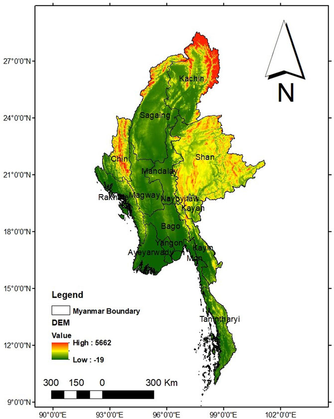
FIGURE 1. Elevation map of Myanmar (mm).

2.2. Datasets

2.2.1 Observed precipitation

Monthly precipitation data at a 0.5 grid resolution (Schneider et al., 2015) from the Global Precipitation Climatology Centre (GPCC) dataset, version 7 (GPCC 2021), are used in this work. The data are available from https://psl.noaa.gov/data/gridded/data.gpcc.htm and have been used and verified with the region’s observed precipitation (Sein et al., 2015; Sein et al., 2021a).

2.2.2 CMIP6 models

The historical experiments of 12 CMIP6 models (Eyring et al., 2016) were obtained from https://esgf-node.llnl.gov/search/cmip6 for the period 1950–2014 (Table 1). All models were resampled to a common grid of 0.5 × 0.5 using bilinear interpolation. Prior to computation, the daily data were aggregated to a monthly basis. The ensemble mean (ENS) of the 12 CMIP6 models has been computed. Details of all the CMIP6 models used in the present work, including the name of the modelling center, their institution’s identity, and horizontal resolution (longitude × latitude), are given in Table 1.

TABLE 1. Details of the CMIP6 GCMs used in this study.

2.2.3 SST

This study investigates the relationship of the SST with each model and the ENS of precipitation at annual and seasonal scales following (Ashok et al., 2007; Vinayachandran et al., 2009). The Extended Reconstructed SST dataset, version 5 [ERSST.v5; Huang et al. (2017)], for the period from 1854 to the present day, is used for this purpose, obtained from the National Oceanic and Atmospheric Administration (NOAA) via https://climatedataguide.ucar.edu/climate-data/sst-data-noaa-extended-reconstruction-ssts-version-5-ersstv5. The horizontal resolution of the data is 2 × 2. The atmospheric circulation pattern is shown using the reanalysis u and v winds that are retrieved from NCEP-NCAR website.

2.1 Materials and methods

2.3.1 Mann–Kendall test

To analyze the trends, this study uses the Mann–Kendall (MK) test (Mann 1945), calculated as follows:

where S is the rating score (called the MK sum), x is the data value, i and j are counters, and n represents the number of data points. Then,

where Var (S) is the standardized variance, and

in which $⃒Z⃒>Z_{\propto /2}$ represents the time series of the data. The significance level is shown by $\propto$ = 0.05, or $Z_{\propto /2}=1.96$, and $⃒Z⃒>1.96$ means a significant trend.

To compute the linear trend rate, the Theil-Sen’s estimator was used based on Eq. 4. Here, note that trend rate values greater than zero (i.e., $∆\sigma$ >0) denotes a positive value (or increasing rate) and trend rate values less than zero (i.e., $∆\sigma$ <0), denotes a negative value (or means decreasing rate).

where the slope between two points is shown as $\beta$; medium represents a function; x_j and x_k correspond to data values for time points j and k (j > k), respectively.

2.3.2 Bilinear interpolation

The bilinear interpolation method uses four 4) known neighboring image coordinates located diagonally from each other to compute the final interpolated value based on the weight of each pixel values from samples. The study followed the general bilinear procedures explained in Bayen et al. (2015). This method was implemented in Climate Data Operators (CDO).

Let assume, the final interpolated value is a function ($f$) at a location $V\left(x,y\right)$.

where $\mathrm{V}\left({\mathrm{x}}_{\mathrm{i}},{\mathrm{y}}_{\mathrm{j}}\right)=U_{ij},i,j=\mathrm{0,1}$. $U_{00}\left(x,t\right),$ $U_{0n}\left(x,t\right),U_{n0}\left(x,y\right)\mathrm{a}\mathrm{n}\mathrm{d}{U}_{mn}\left(x,y\right)$ denotes four (4) known neighboring image coordinates.

2.3.3 Taylor diagram

A Taylor diagram (Taylor et al., 2012) provides a graphical summary of how closely a pattern or set of patterns resembles observations. For more details on the nomenclature of the Taylor diagram, we refer readers to (Taylor et al., 2012). The correlation (r), root mean square error (RMSE), and relative bias (RBIAS) were computed as follows:

where n, X_i and Y_i represent the number of years and the CMIP6 and GPCC series, for example, at time $i$; and $\overline{X}$ and $\overline{Y}$ represent the average of $X_i$ and $Y_i$ for the study period, respectively.

The RMSD stands for root mean square deviation between two variables mainly the predicted (simulated models) and reference (GPCC), which is defined as follows:

The RMSE gives the magnitude of the forecast errors The RMSE is defined as the root mean square error with giving formula:

Where $x_i$ and $x_i^{\prime }$ represent the predicted and reference values, respectively. N is the total number of values in $x_i$ and $x_i^{\prime }$ with $x_i$ and $x_i^{\prime }$ having the same size.

The RBIAS is computed as follows:

where $X_i$ is the simulated precipitation and $Y_i$ is the observed precipitation; $\overline{X}$ and $\overline{Y}$ are the long-term means of precipitation, respectively.

3 Results

3.1 Precipitation variations in GPCP

3.1.1 Annual and seasonal mean climatology

Figure 2 presents the spatial pattern of annual and seasonal precipitation from observation (GPCP) over the period 1970–2014. Figure 2A presents the spatial variations of annual precipitation from GPCP observations over the study area. The annual precipitation results showed a distribution in the range of <100 to >600 mm (Figure 2A). The study observed highest precipitation amount of 450 mmyr⁻¹ (range 300–600 mmyr^-1) occurred the southern region of Mon province and western portions of Rakhine province. In addition, the study observed that the lowest precipitation amount ranges from <50 mmyr⁻¹ in the Mandaley province (in the central region) to 100 mmyr⁻¹ in the Shan province located in the eastern part of the country. We observed distinct spatial patterns in the north (i.e., Kachin and Sagaing province) and southmost (Yangon and Ayeryarwady) part of the study area with values of 150–200 mm year⁻¹.

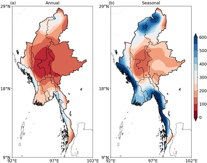
FIGURE 2. Spatial distribution of GPCC precipitation observations for (A) annual (B) seasonal during 1970–2014 (mm).

Figure 2B shows the seasonal (MJJASO) variations in GPCP precipitation observations. The Rakhine (i.e., western region), Yangon Ayeryarwady, Mon, Kayin and Tanintharyi (southmost region), and Kachin (northern region) presented a distinct spatial variation with mean seasonal values ranges from 400 to 600 mm. We observed a distinct decreasing amount from <200 mm in Shan province (eastern region), Naybyitaw, Magwa, Chin to <100 mm in south of Sagaing and Mandalay region.

3.1.2 Trends in annual and seasonal precipitation

Figure 3 presents the trends of the annual and seasonal precipitation over Myanmar during 1970–2014 based on the MK test at the 90% confidence level for the observation (GPCC). The central and eastern parts of the country underwent weakly positive change, whereas the rest of the country shows a negative variation (Figure 3A). The GPCC results show a significant decrease in precipitation over the northwest and east but a significant increase over the Gulf of Martaban. Figure 3B show the MK test is also applied to investigate the linear trends in the seasonal (MJJASO) variation of precipitation. Overall, the GPCC results show a positive (negative) trend in the west and Gulf of Martaban (northwest).

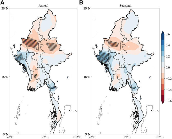
FIGURE 3. MK trend test of GPCC PRE observation for (A) annual and (B) seasonal precipitation. Hatches indicate significance at the 90% confidence level.

3.2 Precipitation variations in CMIP6 models

Figure 4 presents the annual and seasonal cycle of precipitation for the 12 CMIP6 models and the ENS over the region during the period 1970–2014. The ENS exhibits relatively lower precipitation in the western and southern coastal regions but relatively higher precipitation in central and northern regions. The ENS shows higher precipitation over the central region (i.e., Mandalay, lower Sagaing, and Magway) and lower precipitation along the coast (i.e., Rakhine and Mon, Kayin and Tanintharyi). The results of CESM2, CNRM-CM6, MRIESM2-0, and IPSL-CM6A-LR relative to the ENS produces highest precipitation values. The study observed that many of the CMIP6 models are similar—namely, CNRM-ESM2-1, CNRM-CM6, HadGEM3-GC31-LL, MIROC6, CESM2, MRI-ESM2-0, and UKESM1-0-LL—but all except MRI-ESM2-0 also show high precipitation in north and northeast regions. Moreover, similar spatial patterns are observed in GFDL-CM4 and GFDL-ESM4 but with low precipitation occurring in the northwest. MPI-ESM1-2-HR yields low precipitation over the entire region except in the north and deltaic regions.

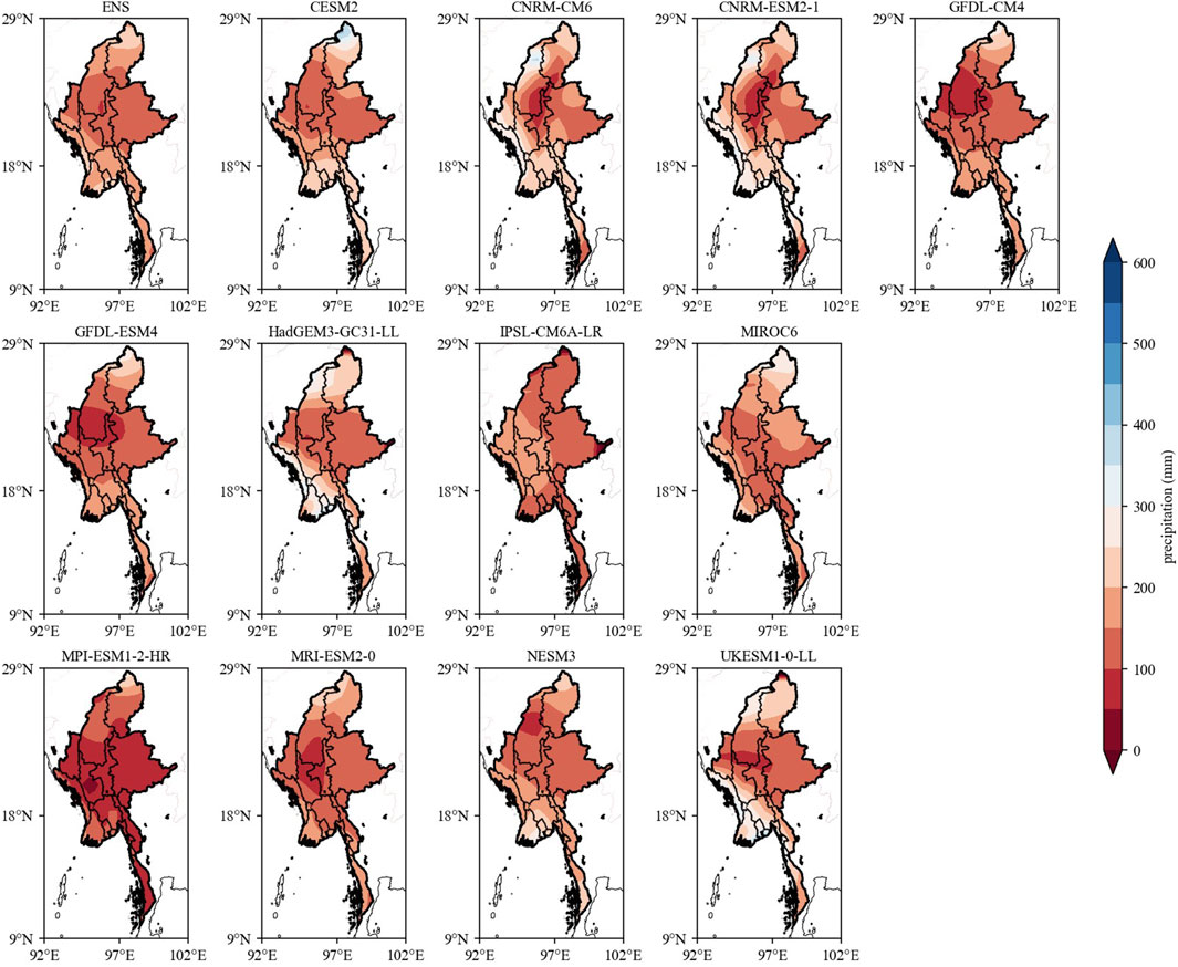
FIGURE 4. Spatial distribution of annual mean precipitation for the selected 12 CMIP6 models as well as their ensemble mean during 1970–2014 (mm).

Figure 5 presents the seasonal cycle of precipitation for 12 CMIP6 models and the ENS during the period 1970–2014. The ENS reveals low precipitation in the central region but high precipitation along the western and southern coastlines and over the Gulf of Martaban. The results of some of the CMIP6 models, such as CNRM-ESM2-1, CNRM-CM6, HadGEM3-GC31-LL and UKESM1-0-LL, presents low precipitation in the central region and high precipitation along the west and south coasts and in the northwest. Meanwhile, GFDL-CM4 and GFDL-ESM4 show low precipitation in the central and northwest regions but high precipitation in the south and at the northern tip. IPSL-CM6A-LR produces high precipitation in central and western regions but low precipitation in the northwest. MIROC6 shows low precipitation in central and northwestern regions but high precipitation in the west, deltaic and northern tip areas. CESM2 presents low (high) precipitation in the central and northwest (north and south) regions. MPI-ESM1-2-HR produces low precipitation in central, eastern and southern areas but high precipitation in the deltaic and northern regions. MRI-ESM2-0 produces low precipitation in the center of the country but high precipitation along the western and southern coasts and in the Andaman Sea. NESM3 shows low (high) precipitation in the east and northwest (deltaic region).

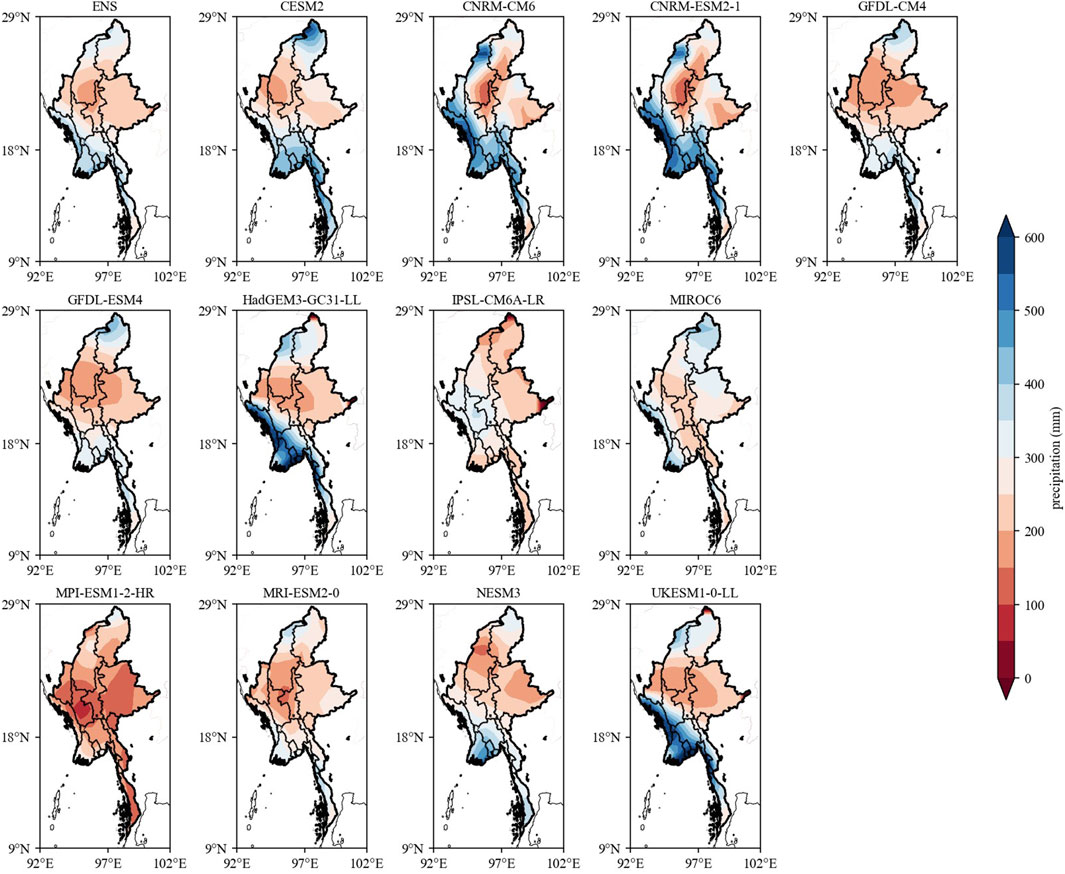
FIGURE 5. Spatial distribution of seasonal mean precipitation for the selected 12 CMIP6 models as well as their ensemble mean during 1970–2014 (mm).

3.2.1 Trends in annual and seasonal CMIP6 precipitation

CNRM-ESM2-1 shows a significant positive precipitation trend over the northwest but a significant negative trend at the northern tip and in the south. GFDL-CM4 presents a significant negative trend in the north, northwest and south. CNRM-CM6 shows a significant negative trend in the center of the country, in the east, in the deltaic region, and in the south. Moreover, GFDL-ESM4 and IPSL-CM6A-LR show a significant negative trend in the south. HadGEM3-GC31-LL produces a significant positive trend in the Bay of Bengal and Gulf of Martaban but a negative trend in the northeast. MIROC6 shows a significant negative trend in the south and in the deltaic region but a significant positive trend in the north. CESM2 produces a significant negative trend in the deltaic region but a significant positive trend in the central part of the country. MPI-ESM1-2-HR presents a significant negative trend in central, eastern, northwestern and southern Myanmar, but a significant positive trend over the Andaman Sea. MRI-ESM2-0 shows a significant negative trend over sea areas (i.e., the Andaman Sea and the eastern and central Bay of Bengal). NESM3 produces a significant positive trend over the northwest and south. UKESM1-0-LL shows a significant positive trend over the west but a negative trend in the north, east and south. And finally, ENS shows a significant positive trend in the northwest but a negative trend in the deltaic, eastern and southern regions.

Similarly, the MK test was also applied to investigate the linear trends in the seasonal (MJJASO) variation of precipitation, based on both the observational data (from GPCC) and the 12 CMIP6 models and their ENS at the 90% confidence level. The results help us to further understand how the different GCMs and observational data capture the precipitation seasonality over this period in Myanmar. The GPCC results show a positive (negative) trend in the west and Gulf of Martaban (northwest). CNRM-ESM2-1 produces a significant positive (negative) trend in the north (south). However, negative trend values can be observed at the northern tip of the country. GFDL-CM4 presents a negative trend in the north and south. CNRM-CM6 (GFDL-ESM4) shows a negative trend over part of the country, mainly in the central, eastern, deltaic and southern regions (west, northwest and south). HadGEM3-GC31-LL shows a negative (positive) trend in the north (east and deltaic area). IPSL-CM6A-LR generates a significant negative trend in southern areas. MIROC6 shows a significant negative trend in the deltaic region and in the south but a significant positive trend in the north. CESM2 yields a significant negative (positive) trend in the west and deltaic (central and northern) regions. MPI-ESM1-2-HR presents a significant negative trend in the eastern, northeastern, central and southern regions, as does MRI-ESM2-0 but only in the eastern region. NESM3 produces a significant positive trend in the north and northwest, and UKESM1-0-LL presents a significant positive (negative) trend in the west (north, east and southern tip) regions.

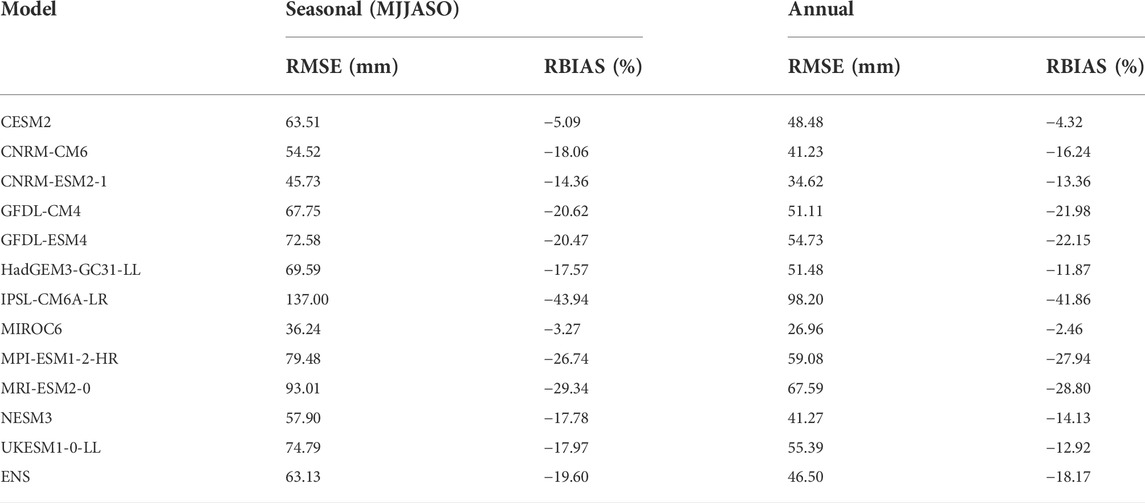
TABLE 2. Root mean square error (RMSE, mm) and relative bias (RBIAS, %) for seasonal (May–October, MJJASO) and annual precipitation in Myanmar during 1970–2014.

3.3 Evaluation of CMIP6 performance against observations

Figure 6 is a Taylor diagram of the annual precipitation over the region simulated by the 12 CMIP6 models relative to the GPCC observations. The simulated pattern of each model is marked with symbols (red and blue). GPCC lies on the positive x-axis, which indicates the reference precipitation data. ENS presents a better correlation coefficient than the other models, with a CC (root-mean-square difference, RMSD) of 0.29 (104 mm). MRI-ESM2-0’s correlation (RMSD) is found to be 0.24 (110 mm), and HadGEM3-GC31-LL’s is 0.13 (113 mm). MPI-ESM1-2-HR shows a CC of 0.26 and RMSD of 106 mm, while CESM2 produces values of 0.23 with 117 mm, respectively. UKESM1-0-LL, CNRM-ESM2-1, GFDL-CM4 and GFDL-ESM4 show CCs of 0.19 (113 mm), 0.21 (108 mm), 0.22 (108 mm), and 0.35 (114 mm). In addition, MIROC6, CNRM-CM6 and NESM3 present a CC (RMSD) of 0.02 (126 mm), 0.21 (120 mm), and 0.33 (117 mm), respectively.

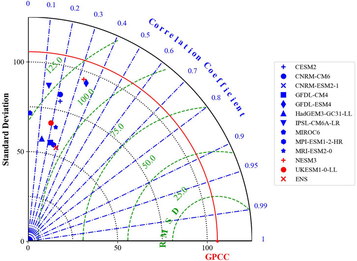
FIGURE 6. Taylor diagram comparing annual (January-December) PRE observation (GPCC) with models (CMIP6).

To evaluate the models’ performances in terms of the mean annual cycle (January–December) of precipitation in Myanmar, as well as that of ENS, we employed some metrics parameters. From the whole models, the RMSEs range from 26.96 to 98.2 mm. The results of the individual models’ RMSE (PCC) are as follows: MIROC6, 26.96 mm (0.93); CNRM-ESM2-1, 34.62 mm (0.97); CNRM-CM6, 41.23 mm (0.98); NESM3, 41.27 mm (0.97); CESM2, 48.48 mm (0.84); GFDL-CM4, 51.11 mm (0.95); HadGEM3-CC31-LL, 51.48 mm (0.85); GFDL-ESM4, 54.73 mm (0.89); UKESM1-0-LL, 55.39 mm (0.80); MPI-ESM1-2-HR, 59.08 mm (0.97); MRI-ESM2-0, 67.59 mm (0.92); IPSL-CM6A-LR, 98.2 mm (0.92). Meanwhile, ENS produces an RMSE of 46.50 mm.

Figure 7 presents the seasonal (MJJASO) precipitation over Myanmar simulated by the CMIP6 models relative to GPCC observations. The ENS shows low RMSD (201 mm) and CC (0.43), indicating the ENS correlation is among the best models that are strongly interconnected with GPCC precipitation. In general, most of the models simulated with good correlation coefficients. For instance, the correlation coefficient along with root mean square deviation is 0.33 (220 mm), 0.35 (223 mm), 0.32 (233 mm), 0.35 (210 mm), 0.36 (210 mm), 0.49 (207 mm), 0.38 (209 mm), 0.40 (206 mm) and 047 (211 mm) for CESM2, CNRM-CM6, CNRM-ESM2-1, GFDL-CM4, GFDL-ESM4, HadGEM3-GC3, MRI-ESM2-O-L, NESM3, and UKESM-O-LL, respectively. Meanwhile, three models such as IPSL-CM6, MIROC6 and MPI-ESM1 presented low correlations along with relatively high deviations from the reference with the values of 0.29 (215 mm), 0.22 (239 mm) and 0.14 (252 mm), respectively; in representing the seasonal precipitation over the region of study. Based on correlation coefficient, the preferred model is HadGEM3 while the ENS presents the lowest deviation from the mean of the reference. The model showing the lowest standard deviation is IPSL-CM followed by the ENS. The low standard deviation indicates the low variability in the model to simulate the observation GPCC precipitation.

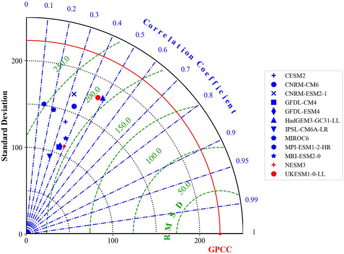
FIGURE 7. Taylor diagram comparing seasonal (MJJASO) PRE observation (GPCC) with models (CMIP6).

Overall, MIROC6, CNRM-ESM2-1, CNRM-CM6, and NESM3 reveal lower RMSEs and higher PCCs. Table 2 lists the RMSE (mm) and RBIAS (%) values for annual rainfall during 1970–2014.

Further analysis of the spatial distribution of the CCs of GPCC precipitation and that of the 12 individual CMIP6 models at the annual scale is shown in Figure 8. The results indicate significant negative (positive) correlation for CESM2-G in the east (south) of the region, for GFDL-ESM4-G in the north and east (deltaic region); for HadGEM3-GC31-LL-G in the west (central and southern regions); and for MPI-ESM1-2-HR-G in the north (central, northwestern and eastern regions). Meanwhile, there is significant positive correlation for CNRM-CM6-G in the south; for GFDL-CM4-G in the central part of the region; for IPSL-CM6A-LR_G in the north, northwest and east; for MIROC6-G in the north and northwest; and for UKESM1-0-LL-G in the north. In addition, there is significant negative correlation for CNRM-ESM2-1-G and MRI-ESM2-0-G in central areas; for NESM3-G in the north and east; and for ENS in the eastern, central and western regions.

FIGURE 8. Spatial distribution of correlation coefficient of annual GPCC PRE with the 12 CMIP6 models. Hatches indicate significance at the 90% confidence level.)

Figure 9 shows the spatial distribution of the CCs between the seasonal (MJJASO) observed (GPCC) precipitation and that of the 12 CMIP6 models. There are negative (positive) CCs for CESM2-G in the east (south); for GFDL-CM4-G in the south (central region); for GFDL-ESM4-G in the north and east (deltaic region); and for MPI-ESM1-2-HR-G in the north (south). Meanwhile, there are positive CCs for CNRM-CM6-G in the south and northwest; for IPSL-CM6A-LR-G in the east and south; and for UKESM1-0-LL-G in the west and east. Moreover, there are negative CCs for CNRM-ESM2-LG in central and southern areas; for HadGEM3-GC31-LL-G in the north, east and west; for MIROC6-G in the northwest and south; for MRI-ESM2-0-G at the northern tip of the country and in central and eastern regions; for NESM3-G in the east; and for ENS in the northeastern, central and western areas. All the results are significant at the 90% confidence level.

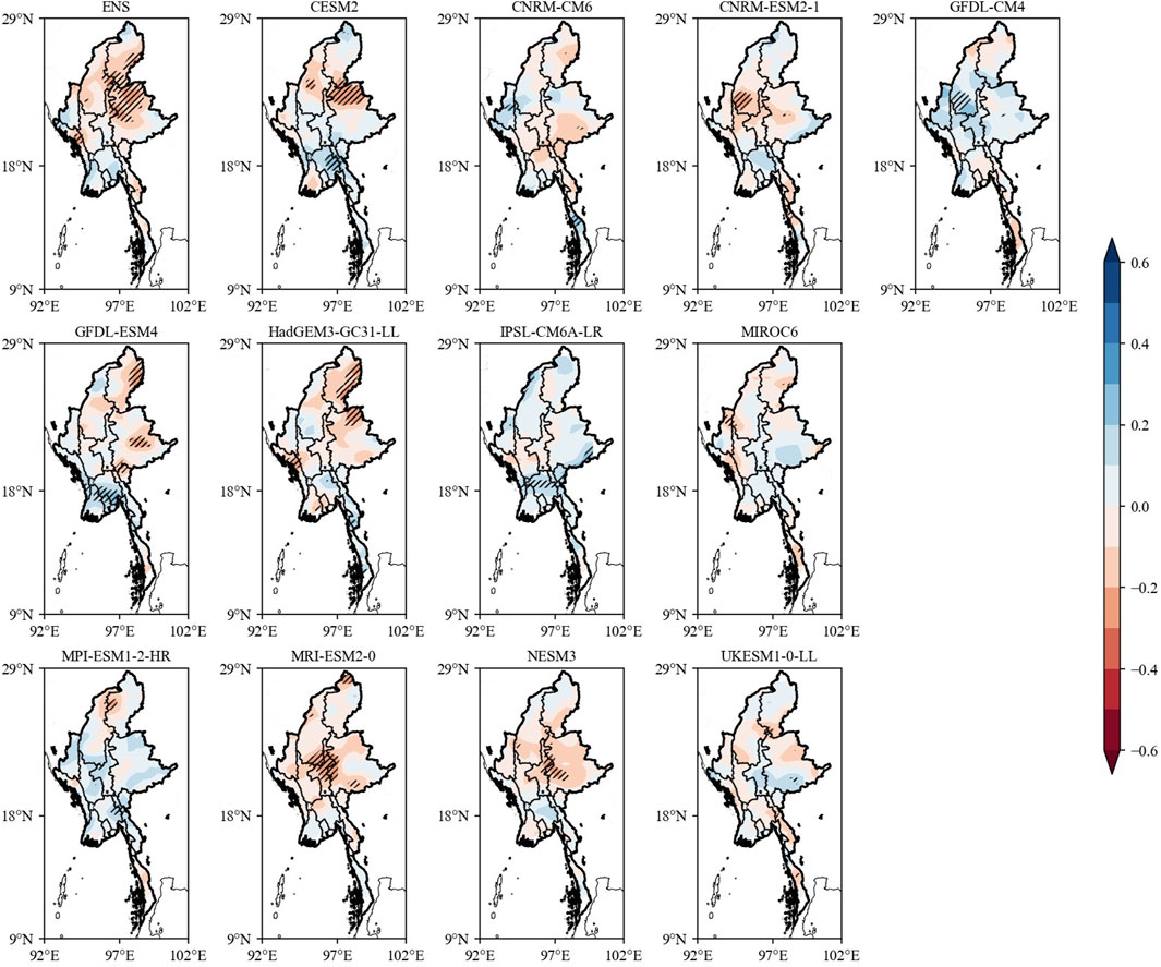
FIGURE 9. Spatial distribution of correlation coefficient of seasonal GPCC PRE (MJJASO) with the 12 CMIP6 models. Hatches indicate significance at the 90% confidence level.

3.4 Relationship between SST and precipitation

The correlation was computed to examine the underlying atmospheric circulation factors (i.e., SST) that influence precipitation variations over the monsoon corridor of Southeast Asia. Specifically, we computed the relationship using simple correlation analysis at the 95% significance level, and the results in terms of the relationship between precipitation (GPCC and ENS) and SST anomalies, globally and in the Myanmar region, are shown in Figure 10 (for GPCC) and Figure 10 (for ENS) at the annual and seasonal scales.

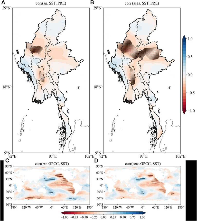
FIGURE 10. Spatial distributions of (A,C) correlation coefficients of GPCC PRE (i.e., annual and seasonal) and SST during 1970-2014). (A) GPCC-annual (B)Region GPCC-annual (C) GPCC -seasonal and (D) Region GPCC -seasonal. Hatched area indicates 95% confidence level.

Figure 10A shows negative (low) correlation between annual observed (GPCC) precipitation and SST over the northeastern, central and southeastern Pacific Ocean but positive (high) correlation over the northwestern and southwestern Pacific Ocean. Moreover, the Indian Ocean shows negative (low) correlation east of Africa extending north and east of Madagascar. In Myanmar, there is negative (low) correlation in central, northwestern and eastern areas (Figure 10B). For seasonal (MJJASO) GPCC precipitation and SST, the annual spatial pattern of their correlation is similar, but with weaker negative correlation over the central Pacific Ocean than at the annual scale (Figure 10C). In addition, negative (low) correlation over central and northwest Myanmar is shown in Figure 10D.

Figure 11A shows negative correlation between annual simulated (ENS) precipitation and SST over the northeastern and southeastern Pacific Ocean but positive correlation over the northwestern, southwest and southeastern Pacific Ocean. However, the spatial distribution in the Indian Ocean does not show any significant correlation. In Myanmar, there is significant negative (positive) correlation in the south (northwest) of the region (Figure 11B). Seasonally (MJJASO), Figure 11C shows positive (negative) CCs in the northwest (northeast) Pacific Ocean, but weaker than at the annual scale. Regionally (i.e., in Myanmar), positive (negative) CCs are apparent in the northwest (south and at the northern tip) of the country (Figure 11D).

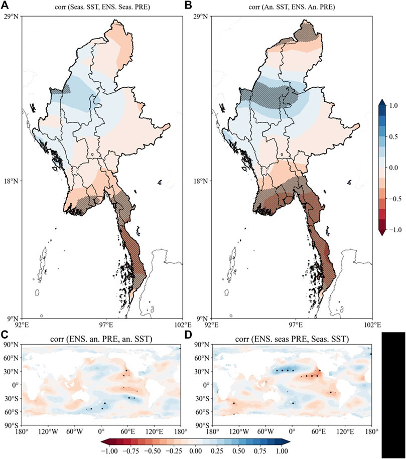
FIGURE 11. Spatial distribution of the correlation coefficients between ENS PRE (annual and seasonal) and SST during 1970-2014. (A) ENS-annual (B) Region ENS-annual (C) ENS-seasonal and (D) Region ENS-seasonal. Hatched area indicates 95% confidence level.

Overall, the GPCC and ENS results show negative (positive) correlation in the northeastern, central and southeastern (northwestern and southwestern) Pacific Ocean, with ENS showing a similar spatial pattern of CCs to GPCC, albeit with weaker negative (positive) correlation in the central (southern) Pacific Ocean in ENS. In addition, ENS does not perform well in the Indian Ocean. In Myanmar, at the annual scale, GPCC shows negative correlation over central, eastern and northwestern parts, while at the seasonal (MJJASO) scale it is in only in the central and northwestern areas (Figure 11). Meanwhile, ENS, both at the annual and seasonal (MJJASO) scale, shows negative (positive) correlation in the south (northwest), but negative correlation over the northern tip of the region at the seasonal scale only (Figure 11).

Circulations of two atmospheric variables over Myanmar for the period of study are depicted by Figure 12. A low large center (negative pressure vertical velocity) is developed between 950 hope and 100 hpa within about 5 N–10 N. Meanwhile, two high centers (positive pressure vertical velocity) are found at upper and lower atmosphere around 25 N as shown by the red arrows pointing down (Figure 12A). The negative center indicates a rising motion (i.e., green arrows pointing up), which favors the precipitation, whereas the positive center corresponds with descending motion that involve the dry period. The climatology of winds circulations over is featured by southwesterly with a high center found in southern part of the country (Figure 12B).

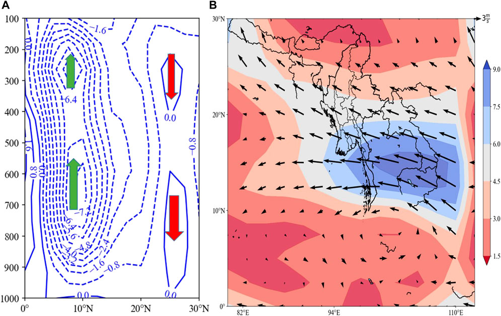
FIGURE 12. Mean of (A) pressure vertical velocity and (B) winds circulation for the period from 1970 to 2014. Arrows in green and pointing up indicates rising motion and arrows in red pointing down indicates descending motion while the shaded represents the wind speed.

4 Discussion

This study uses 12 state-of-the-art GCMs from CMIP6 to investigate the precipitation patterns across Myanmar at different spatial and temporal scales during the period 1970–2014, as well as the trends and potential drivers. The performances of the 12 individual models and their ENS in reproducing the historical precipitation is evaluated against GPCC observations. Overall, at the annual scale, IPSL-CM6A-LR, MRI-ESM2-0 and HadGEM3-GC31-LL present high correlation and relatively lower RMSDs (Figure 2). In contrast, CESM2, UKESM1-0-LL, CNRM-ESM2-1 and GFDL-CM4 show low to no correlation and relatively higher RMSD. Meanwhile, MIROC6, CNRM-CM6 and NESM3 perform poorly over the region, with negative correlation (Figure 2). The PCCs of the individual models and their ENS range from 0.8 to 0.97, and the RMSE from 26.96 to 98.2 mm (Figure 3). The seasonal (MJJASO) results of the CMIP6 models relative to GPCC observations were also investigated, revealing that IPSL-CM6A-LR performs better than GFDL-CM4, MPI-ESM1-2-HR, NESM3, MRI-ESM2-0, CNRM-CM6, and HadGEM3-GC31-LL. Meanwhile, CESM2 shows no correlation, and GFDL-ESM4, CNRM-ESM2-1 and MIROC6 show negative and low correlation values (Figure 4). The seasonal precipitation analysis showed that IPSL-CM6A-LR produces a lower RMSE (9.0 mm) and CC (0.3) than the rest of the individual models (Figure 5).

The performances of the models in terms of the mean annual cycle of precipitation were also evaluated, using PCCs, with all models showing high PCC values of >0.80. ENS outperforms the individual models, except for MIROC6, CNRM-ESM2-1, and CNRM-CM6. Similar results were found in the seasonal analysis (Figures 4, 5). The RMSEs of the CMIP6 models and their ENS (Figures 4, 5) reflect the differences between them and the GPCC observations. The four (“best”) models with RMSEs lower than the ENS value of 46.50 mm/yr were chosen, and these four best models at the annual scale were MIROC6, CNRM-ESM2-1, CNRM-CM6, and NESM3. The remaining models—CESM2, GFDL-CM4, HadGEM3-CC31-LL, GFDL-ESM4, UKESM1-0-LL, MPI-ESM1-2-HR, MRI-ESM2-0, and IPSL-CM6A-LR—show slightly higher RMSE. Similarly, the same models were selected for seasonal values (Figure 5) based on the RMSEs of individual models being lower than the ENS value of 63.13 mm. The differences in the results of individual models might be related to the uncertainty in their simulations, which may stem from inherent model biases and other sources, as stipulated by (Taylor et al., 2012; Eyring et al., 2016).

The climatological results in Figure 13 show that the 12 CMIP6 models and their ENS present similar spatial and temporal patterns of annual precipitation over Myanmar to those of GPCC. The results show that the western and southern coastal regions receive the most precipitation, with central areas receiving the least (Sein et al., 2015; Sein et al., 2021a; Sein et al., 2022). In terms of the interannual and seasonal variations in Myanmar, GPCC and the individual models (except for MRI-ESM2-0) show similarity insofar as they both present high precipitation in the north and northeast regions. MPI-ESM1-2-HR reveals low precipitation in the entire region, except in the north and deltaic area. IPSL-CM6A-LR shows an opposite pattern to the precipitation gradient of GPCC, and ENS exhibits relatively low (high) precipitation in the central (coastal and northern) regions.

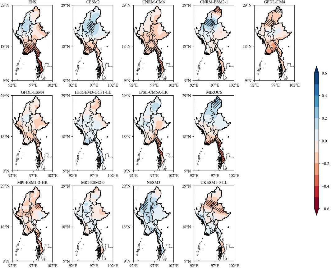
FIGURE 13. MK trend test of annual precipitation for the selected 12 CMIP6 models, and ENS. Hatches indicate significance at the 90% confidence level.

The annual mean precipitation climatology over Myanmar was also investigated (Figure 14), revealing a strong temporal variability over the region. The low precipitation in February and peak in July, captured by both GPCC and the GCMs, is consistent with the climatology of the region. The highest (lowest) precipitation is recorded by CESM2 (IPSL-CM6A-LR) (Figure 14). Meanwhile, CNRM-CM6, MRIESM2-0, IPSL-CM6A-LR, GPCC and ENS show a higher precipitation peak in July (Figure 14) than the rest of the models. The ENS results reproduce the region’s climatology well, and better than the individual models. The performance of ENS over individual models in terms of precipitation simulation is consistent with a previous study (Xu and Xu 2012).

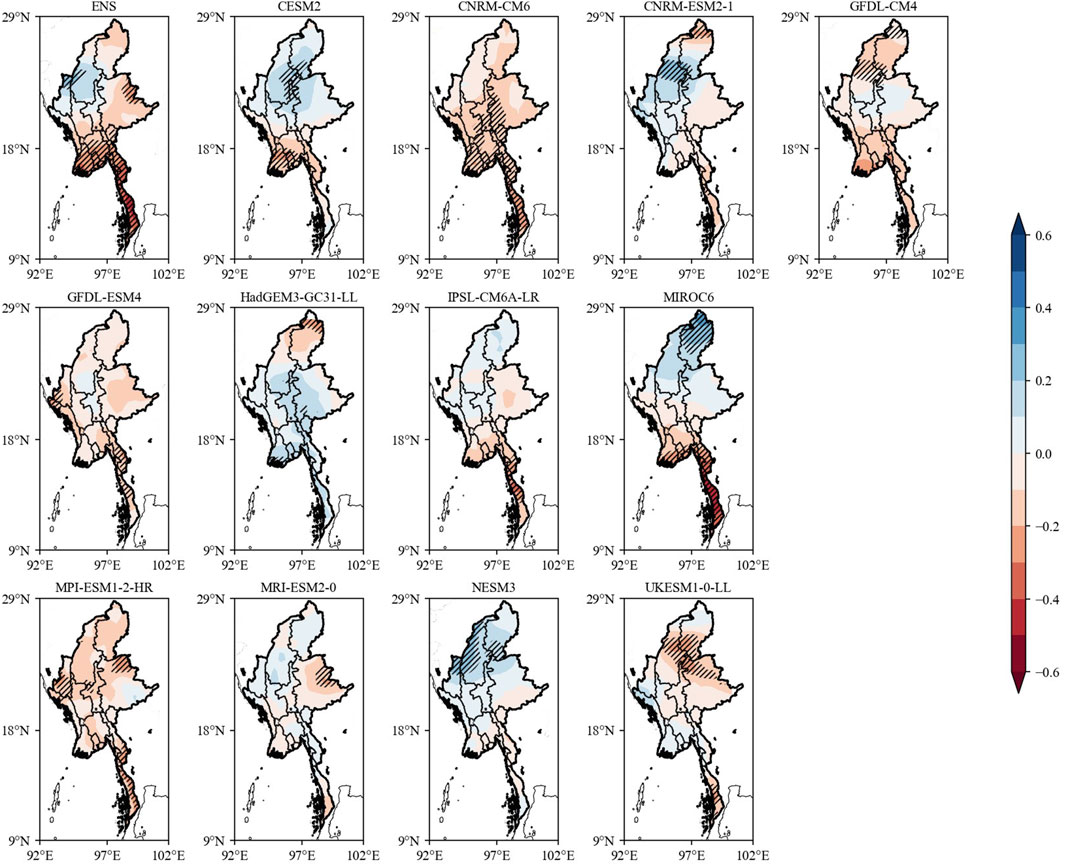
FIGURE 14. MK trend test of seasonal (MJJASO) precipitation for the selected 12 CMIP6 models and ENS. Hatches indicate significance at the 90% confidence level.

Using linear trend analysis to assess the 12 CMIP6 models, five models were selected for Myanmar to show the significant trend in precipitation in northern Myanmar, including the northeast and northwest (Figure 15)—namely, CNRM-ESM2-1, GFDL-CM4, CNRM-CM6, GFDL-ESM4, and IPSL-CM6A-LR. The west, center and east of Myanmar are shown in HadGEM3-GC31-LL, MIROC6, CESM2, MPI-ESM1-2-HR, MRI-ESM2-0, NESM3, and UKESM1-0-LL to have low but significant trends. These results suggest that these models capture the precipitation seasonality over the study period in Myanmar consistently with previous studies in the Southeast Asian region (Kumar et al., 2013).

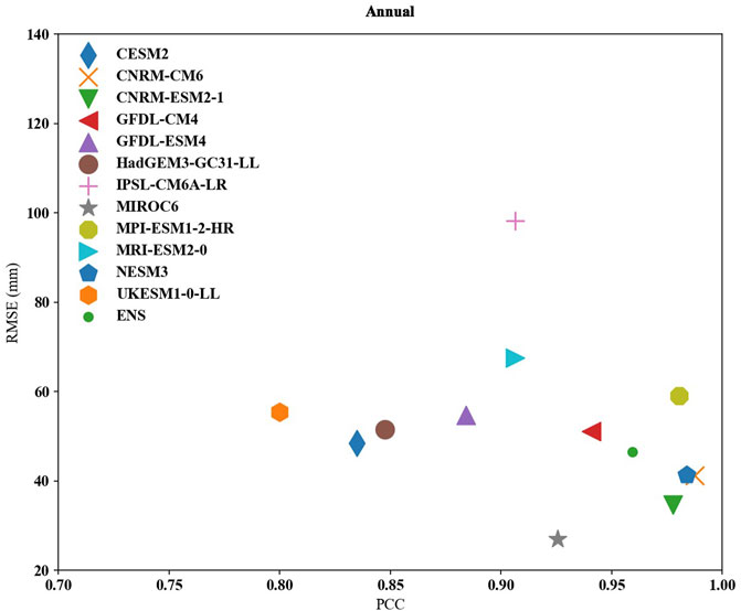
FIGURE 15. Performance of mean annual cycle PRE (mm) for CMIP6 models and their multimodal ensemble mean (ENS) on PRE climatology (1970-2014). The abscissa and ordinates are pattern correlation coefficient (PCC) and root mean square error (RMSE), respectively.

The relationship between precipitation and SST investigated the link between summer monsoon precipitation and global-scale SST. A simple correlation was performed for the ENS and global SST, and the annual ENS precipitation and SST were analyzed over the Pacific Ocean. Significant negative correlation was found across the northeast and southeast parts of the Pacific Ocean, while positive correlation was found across the northwest, southwest and southeast parts. Similarly, the seasonal (MJJASO) ENS precipitation and SST showed positive (negative) CCs in the northwest (northeast) Pacific Ocean, but weaker than at the annual scale in the southern Pacific. No significant correlation was recorded for the Indian Ocean. Generally, for ENS, the annual and seasonal correlation between SST and precipitation was found to be negative (positive) in the south (northwest), but ENS shows negative seasonal correlation in the northern tip of the region (Figure 11). The circulation results of the two atmospheric variables (Figure 12) shown low large center (negative pressure vertical velocity) is developed between 950 hope and 100hpa within about 5 N to 10 N. Two high centers (positive pressure vertical velocity) are found at upper and lower atmosphere around 25 N as shown by the red arrows pointing down (Figure 12A). The negative center indicates a rising motion (i.e., green arrows pointing up), which favors the precipitation, whereas the positive center corresponds with descending motion that involve the dry period. The climatology of winds circulations over is featured by southwesterly with a high center found in southern part of the country (Figure 12B). In summary, the use of the latest GPCC observations and CMIP6 model data shows the ability of GCMs to reproduce well the patterns of seasonal precipitation in Myanmar, consistent with previous studies across the region, with high PCCs and lower RMSE.

5 Conclusion

In the present study, the individual and collective (i.e., ENS) performances of 12 GCMs from CMIP6 in capturing the precipitation pattern over Myanmar for the period 1970–2014 were analyzed. More specifically, the GCM precipitation was compared with that of observations from GPCC through displaying the climatology at annual and seasonal scales and the interannual variability. In addition, skill scores were used for statistical evaluation. Moreover, the relationship between the time series of GPCC and ENS was examined to uncover how the precipitation is controlled by the variability of SST over Myanmar through the tele-connectivity of atmospheric parameters. The main conclusions can be summarized as follows:

1) Among the 12 CMIP6 models, only MPI-ESM1-2-HR is able to roughly reproduce the GPCC precipitation pattern over Myanmar during 1970–2014 at both annual and seasonal scales. Meanwhile, at the interannual scale, most models underestimate the monthly precipitation, except CESM2, which overestimates that of GPCC from July to December. Furthermore, 3 out of the 12 models fail to capture the peak precipitation in July.

2) The RMSE of ENS produces an annual value of 46.50 mm and seasonal value of 63.13 mm. The RBIAS is −18.17 and −19.60 at the annual and seasonal scale over Myanmar, respectively.

3) MIROC6, CNRM-ESM2-1, CNRM-CM6, and NESM3 show lower RMSEs than the ENS value. The remaining models (CESM2, GFDL-CM4, HadGEM3-CC31-LL, GFDL-ESM4, UKESM1-0-LL, MPI-ESM1-2-HR, MRI-ESM2-0, and IPSL-CM6A-LR) show slightly higher RMSE.

4) Linear trend analysis shows that CNRM-CM6, GFDL-ESM4, GFDL-CM4, IPSL-CM6A-LR, and CNRM-ESM2-1 produce a significant positive trend in capturing the precipitation seasonality over the study period in Myanmar. HadGEM3-GC31-LL, MIROC6, CESM2, MPI-ESM1-2-HR, MRI-ESM2-0, NESM3, and UKESM1-0-LL show significant negative trends.

5) The ENS (annual and seasonal) correlation between precipitation and SST is negative (positive) in the south (northwest), but the ENS seasonal correlation is negative over the northern tip of the region.

Based on these results, we recommend further studies consider simulating the precipitation changes over Myanmar to provide more information toward a better understanding and ability to project future precipitation changes in this region.

Data availability statement

The original contributions presented in the study are included in the article/Supplementary Material, further inquiries can be directed to the corresponding author.

Author contributions

ZS and XZ: conceptualization, methodology, investigation, writing-original draft, writing-review and editing, resources, supervision. FO, IN, and KP: conceptualization, data curation, writing-review and editing. ZS, XZ, FO, IN, and KP were all involved in the scientific interpretation and discussion. All authors provided commentary on the paper.

Funding

This work was jointly supported by the National Key Research and Development Program of China (2017YFC1502000) and the National Basic Research Program of China (2012CB955204).

Acknowledgments

We are grateful to the Collaborative Innovation Centre on the Forecast and Evaluation of Meteorological Disasters, Key Laboratory of Meteorological Disasters, Ministry of Education, Nanjing University of Information Science and Technology, Nanjing, China. Special appreciation goes to the World Climate Research Programme (WCRP) for the provision of the datasets used in the study.

Conflict of interest

The authors declare that the research was conducted in the absence of any commercial or financial relationships that could be construed as a potential conflict of interest.

Publisher’s note

All claims expressed in this article are solely those of the authors and do not necessarily represent those of their affiliated organizations, or those of the publisher, the editors and the reviewers. Any product that may be evaluated in this article, or claim that may be made by its manufacturer, is not guaranteed or endorsed by the publisher.

References

Alexander, L. V. (2016). Global observed long-term changes in temperature and precipitation extremes: A review of progress and limitations in IPCC assessments and beyond. Weather Clim. Extrem. 11, 4–16. doi:10.1016/j.wace.2015.10.007
Amato, R., Steptoe, H., Buonomo, E., and Jones, R. (2019). High-resolution history: Downscaling China’s climate from the 20CRv2c reanalysis. J. Appl. Meteorol. Climatol. 58, 2141–2157. doi:10.1175/jamc-d-19-0083.1
Ashok, K., Behera, S. K., Rao, S. A., Weng, H., and Yamagata, T. (2007). El niño modoki and its possible teleconnection. J. Geophys. Res. 112 (C11), C11007. doi:10.1029/2006jc003798
Babar, Z. A., Zhi, X., and Fei, G. (2014). Precipitation assessment of Indian summer monsoon based on CMIP5 climate simulations. Arab. J. Geosci. 8, 4379–4392. doi:10.1007/s12517-014-1518-4
Bayen, A. M., and Siauw, T. (2015). “An introduction to MATLAB® programming and numerical methods for engineers,” in An introduction to MATLAB® programming and numerical methods for engineers (Boston: Academic Press).
Department of Disaster Managemen (2020). Country report 2020. Avaliable At: https://www.adrc.asia/countryreport/MMR/2020/MMR_CR2020.pdf.
Dong, T.-Y., Dong, W.-J., Guo, Y., Chou, J.-M., Yang, S.-L., Tian, D., et al. (2018). Future temperature changes over the critical Belt and Road region based on CMIP5 models. Adv. Clim. Change Res. 9 (1), 57–65. doi:10.1016/j.accre.2018.01.003
Eckstein, D., Künzel, V., and Schäfer, L. (2020). Global climate risk index 2021. Who suffers most from extreme weather events?. Bonn, Germany: Think Tank & Research.
Eyring, V., Bony, S., Meehl, G. A., Senior, C. A., Stevens, B., Stouffer, R. J., et al. (2016). Overview of the coupled model Intercomparison project Phase 6 (CMIP6) experimental design and organization. Geosci. Model. Dev. 9 (5), 1937–1958. doi:10.5194/gmd-9-1937-2016
Fremme, A., and Sodemann, H. (2019). The role of land and ocean evaporation on the variability of precipitation in the Yangtze River valley. Hydrol. Earth Syst. Sci. 23 (6), 2525–2540. doi:10.5194/hess-23-2525-2019
Ge, F., Zhu, S., Luo, H., Zhi, X., and Wang, H. (2021). Future changes in precipitation extremes over southeast Asia: Insights from CMIP6 multi-model ensemble. Environ. Res. Lett. 16, 024013. doi:10.1088/1748-9326/abd7ad
Ge, F., Zhu, S., Peng, T., Zhao, Y., Sielmann, F., Fraedrich, K., et al. (2019). Risks of precipitation extremes over southeast Asia: Does 1.5 °C or 2 °C global warming make a difference? Environ. Res. Lett. 14, 044015. doi:10.1088/1748-9326/aaff7e
GPCC (2021). Global precipitation climatology Centre) datasets version 7. AvaliableAt: https://opendata.dwd.de/climate_environment/GPCC/html/fulldata_ v7 doi download.html.
He, W.-p., and Zhao, S.-s. (2018). Assessment of the quality of NCEP-2 and CFSR reanalysis daily temperature in China based on long-range correlation. Clim. Dyn. 50 (1), 493–505. doi:10.1007/s00382-017-3622-0
Horton, R., De Mel, M., Peters, D., Lesk, C., Bartlett, R., Helsingen, H., et al. (2017). Assessing climate risk in Myanmar: Summary for policymakers and planners. New York, NY, USA: Center for Climate Systems Research at Columbia University.
Huang, B., Thorne, P. W., Banxon, V. F., Boyer, T., Chepurin, G., Lawrimore, J. H., et al. (2017). Extended reconstructed Sea surface temperature version 5 (ERSSTv5), upgrades, validations, and intercomparisons. J. Clim. 30, 8179–8205. doi:10.1175/JCLI-D-16-0836.1
IPCC (2021). “Summary for policymakers,” in Climate change 2021, the physical science basis contribution of working group I to the sixth assessment report of the intergovernmental panel on climate change (Cambridge, UK: Cambridge University Press).
Iqbal, Z., Shahid, S., Ahmed, K., Ismail, T., and Nawaz, N. (2019). Spatial distribution of the trends in precipitation and precipitation extremes in the sub-Himalayan region of Pakistan. Theor. Appl. Climatol. 137 (3), 2755–2769. doi:10.1007/s00704-019-02773-4
Iqbal, Z., Shahid, S., Ahmed, K., Ismail, T., Ziarh, G. F., Chung, E.-S., et al. (2021). Evaluation of CMIP6 GCM rainfall in mainland Southeast Asia. Atmos. Res. 254, 105525. doi:10.1016/j.atmosres.2021.105525
Jiang, Z. H., Ding, Y. G., and Chen, W. L. (2007). Projection of precipitation extremes for the 21st Century over China. Adv. Clim. Chang. Res. 3, 202–207.
Jiang, Z. H., Song, J., Li, L., Chen, W. L., Wang, Z. F., and Wang, J. (2012). Extreme climate events in China: IPCC-AR4 model evaluation and projection. Clim. Change 110, 385–401. doi:10.1007/s10584-011-0090-0
Kitoh, A., Endo, H., Krishna Kumar, K., Cavalcanti, I. F. A., Goswami, P., and Zhou, T. (2013). Monsoons in a changing world: A regional perspective in a global context. J. Geophys. Res. Atmos. 118, 3053–3065. doi:10.1002/jgrd.50258
Kumar, S., Merwade, V., Kinter, J. L., and Niyogi, D. (2013). Evaluation of temperature and precipitation trends and long-term persistence in CMIP5 twentieth century climate simulations. J. Clim. 26, 4168–4185. doi:10.1175/jcli-d-12-00259.1
Meehl, G. A., Moss, R., Taylor, K. E., Eyring, V., Stouffer, R. J., Bony, S., et al. (2014). Climate model intercomparisons: Preparing for the next Phase. Eos Trans. AGU. 95 (9), 77–78. doi:10.1002/2014eo090001
NECC (2012). MECF Myanmar’s national adaptation Programme of action (NAPA) to climate change. Haverhill, MA, USA: NECC.
O'Neill, B. C., Tebaldi, C., van Vuuren, D. P., Eyring, V., Friedlingstein, P., Hurtt, G., et al. (2016). The scenario model Intercomparison project (ScenarioMIP) for CMIP6. Geosci. Model. Dev. 9 (9), 3461–3482. doi:10.5194/gmd-9-3461-2016
OCHA (2021). Myanmar humanitarian. AvaliableAt: https://reliefweb.int/report/myanmar/myanmar-humanitarian-update-no-9-30-july-2021.
Oo, S. S., Hmwe, K. M., Aung, N. N., Su, A. A., Soe, K. K., Mon, T. L., et al. (2020). Diversity of insect pest and predator species in monsoon and summer rice fields of taungoo environs, Myanmar. Adv. Entomol. 03, 117–129. doi:10.4236/ae.2020.83009
Ren, Y.-Y., Ren, G., Sun, X., Shrestha, A., Zhan, Y., Rajbhandari, R., et al. (2017). Observed changes in surface air temperature and precipitation in the Hindu Kush Himalayan region over the last 100-plus years. Adv. Clim. Change Res. 8, 148–156. doi:10.1016/j.accre.2017.08.001
Schneider, U., Becker, A., Finger, P., Meyer-Christoffer, A., Rudolf, B., and Ziese, M. (2015). GPCC full data monthly product version 7.0 at 0.5°: Monthly land-surface precipitation from rain-gauges built on GTS-based and historic data. Earth Syst. Sci. Data 6, 49–60. doi:10.5194/essd-6-49-2014
Sein, Z., Ogwang, B., Ongoma, V., Ogou, F., and Batebana, K. (2015). Inter-annual variability of summer monsoon rainfall over Myanmar in relation to IOD and ENSO. J. Environ. Agric. Sci. 2313–8629 4, 28–36.
Sein, Z. M. M., Ullah, I., Saleem, F., Zhi, X., Syed, S., and Azam, K. (2021a). Interdecadal variability in Myanmar rainfall in the monsoon season (May–October) using eigen methods. Water 13, 729. doi:10.3390/w13050729
Sein, Z. M. M., Zhi, X., Ullah, I., Azam, K., Ngoma, H., Saleem, F., et al. (2022). Recent variability of sub-seasonal monsoon precipitation and its potential drivers in Myanmar using in-situ observation during 1981–2020. Int. J. Climatol. 42 (6), 3341–3359. doi:10.1002/joc.7419
Stouffer, R. J., Eyring, V., Meehl, G. A., Bony, S., Senior, C., Stevens, B., et al. (2017). CMIP5 scientific gaps and recommendations for CMIP6. Bull. Am. Meteorological Soc. 98 (1), 95–105. doi:10.1175/bams-d-15-00013.1
Taylor, K. E., Stoufer, R. J., and Meehl, G. A. (2012). An overview of CMIP5 and the experiment design. Bull. Am. Meteorol. Soc. 93, 485–498. doi:10.1175/bams-d-11-00094.1
Vinayachandran, P. N., Francis, P. A., and Rao, S. A. (2009). Indian ocean dipole: Processes and impacts. Curr. Trends Sci. 46 (10), 569–589.
Wang, N., Zeng, X.-M., Guo, W.-D., Chen, C., You, W., Zheng, Y., et al. (2018). Quantitative diagnosis of moisture sources and transport pathways for summer precipitation over the mid-lower Yangtze River Basin. J. Hydrology 559, 252–265. doi:10.1016/j.jhydrol.2018.02.003
Keywords: CMIP6, Taylor diagram, correlational analysis, GPCC, climate change, precipitation, Myanmar
Citation: Sein ZMM, Zhi X, Ogou FK, Nooni IK and Paing KH (2022) Evaluation of coupled model intercomparison project phase 6 models in simulating precipitation and its possible relationship with sea surface temperature over Myanmar. Front. Environ. Sci. 10:993802. doi: 10.3389/fenvs.2022.993802
Received: 14 July 2022; Accepted: 25 October 2022;
Published: 15 November 2022.
Edited by:
Wei Shui, Fuzhou University, ChinaReviewed by:
Jianqi Zhang, National University of Defense Technology, ChinaHaijun Deng, Fujian Normal University, China
Copyright © 2022 Sein, Zhi, Ogou, Nooni and Paing. This is an open-access article distributed under the terms of the Creative Commons Attribution License (CC BY). The use, distribution or reproduction in other forums is permitted, provided the original author(s) and the copyright owner(s) are credited and that the original publication in this journal is cited, in accordance with accepted academic practice. No use, distribution or reproduction is permitted which does not comply with these terms.
*Correspondence: Xiefei Zhi, zhi@nuist.edu.cn