Spatial Heterogeneity of eDNA Transport Improves Stream Assessment of Threatened Salmon Presence, Abundance, and Location
 Zachary T. Wood1,2*†
  Lacoursière-Roussel Anaïs3,5*†
  Francis LeBlanc4
  Marc Trudel3 Michael T. Kinnison1,2
  Colton Garry McBrine5 Scott A. Pavey5 Nellie Gagné4
- 1The University of Maine School of Biology and Ecology, Orono, ME, United States
- 2Maine Center for Genetics in the Environment, Orono, ME, United States
- 3St. Andrews Biological Station, Fisheries and Oceans Canada, St Andrews, NB, Canada
- 4Atlantic Science Enterprise Centre, Fisheries and Oceans Canada, Moncton, NB, Canada
- 5Biological Sciences, Canadian Rivers Institute, University of New Brunswick, Saint John, NB, Canada
The integration of environmental DNA (eDNA) within management strategies for lotic organisms requires translating eDNA detection and quantification data into inferences of the locations and abundances of target species. Understanding how eDNA is distributed in space and time within the complex environments of rivers and streams is a major factor in achieving this translation. Here we study bidimensional eDNA signals in streams to predict the position and abundance of Atlantic salmon (Salmo salar) juveniles. We use data from sentinel cages with a range of abundances (3–63 juveniles) that were deployed in three coastal streams in New Brunswick, Canada. We evaluate the spatial patterns of eDNA dispersal and determine the effect of discharge on the dilution rate of eDNA. Our results show that eDNA exhibits predictable plume dynamics downstream from sources, with eDNA being initially concentrated and transported in the midstream, but eventually accumulating in stream margins with time and distance. From these findings we developed a fish detection and distribution prediction model based on the eDNA ratio in midstream versus bankside sites for a variety of fish distribution scenarios. Finally, we advise that sampling midstream at every 400 m is sufficient to detect a single fish at low velocity, but sampling efforts need to be increased at higher water velocity (every 100 m in the systems surveyed in this study). Studying salmon eDNA spatio-temporal patterns in lotic environments is essential to developing strong quantitative population assessment models that successfully leverage eDNA as a tool to protect salmon populations.
Introduction
Recent advances in the collection and analysis of extra-organismal environmental DNA (eDNA) provide a novel indirect approach that can fill gaps in large-scale fish distribution assessments, complementing logistically difficult traditional methods. In addition to improving power of detection, eDNA promises to augment current fish abundance estimates, increasing their precision and accuracy (Lacoursière-Roussel et al., 2015; Doi et al., 2017; Levi et al., 2019). Collecting water samples for eDNA surveys is non-invasive and, in contrast to direct organismal surveys, does not impose any stress on the studied organisms (Dolan and Miranda, 2004; Rummer and Bennett, 2005; Miranda and Kidwell, 2010). Using eDNA to detect and quantify aquatic populations has the power to drastically improve our knowledge of the large- and fine-scale spatial distribution of animals (Lacoursière-Roussel et al., 2016a; Yates et al., 2019). Although a number of studies have started to address the effects of environmental conditions [e.g., water temperature (Lacoursière-Roussel et al., 2016b), the ecology of species (e.g., life stage; Gibson et al., 2003), and eDNA hydrodynamics (Deiner and Altermatt, 2014; Jerde et al., 2016; Wood et al., 2020)], more work is needed to refine models and facilitate the integration of eDNA into conservation and fisheries management decision-making (Barnes et al., 2014; Barnes and Turner, 2016; Sepulveda et al., 2021).
Environmental DNA has three hierarchical potential uses for broadly examining single species: (1) detection, determining the large-scale spatial distribution of a species; (2) quantification, determining the population size in a system based on the eDNA concentration or detection rates, and (3) quantitative distribution assessment, localizing high or low concentrations of organisms to particular geographic locations based on eDNA variability. To date, most eDNA applications have focused on species detection, and few have focused on examining system-wide quantification (Yates et al., 2019). In lotic habitats (rivers and streams), fine-scale population quantification and quantitative distribution assessment are currently limited by our ability to translate eDNA distribution to upstream fish distributions. eDNA distribution is impacted by the physical properties of the stream, e.g., morphology and hydrodynamics (Dejean et al., 2011; Deiner and Altermatt, 2014; Jane et al., 2015). Despite the advantages of lotic eDNA surveys over traditional electric and net surveys in terms of person-power, cost, and potential harm to study organisms, implementation for management could be substantially improved by better characterizing of lotic eDNA dynamics that influence eDNA-based detection, quantification, and distribution assessment of aquatic species.
Examining eDNA in Streams
Despite the huge potential of eDNA for aquatic population management, there is no current model able to accurately and precisely predict upstream fish location or abundance based on lotic eDNA concentrations alone, particularly if eDNA is collected in a limited number of stream locations. In riverine systems, eDNA concentrations exhibit high variability in space and time as eDNA moves downstream from sources (Deiner et al., 2016; Shogren et al., 2016; Wilcox et al., 2016; Sansom and Sassoubre, 2017; Wood et al., 2020). Furthermore, due to the complexity of eDNA states (e.g., tissues, cells, and DNA fragments), eDNA movement is more complex than a conservative tracer or monodispersed solution (Wilcox et al., 2016; Shogren et al., 2017; Pont et al., 2018). Sansom and Sassoubre (2017) presented the first model of downstream eDNA transport based on a simplified longitudinal eDNA decay rate constant. In a marine system, Akatsuka et al. (2018) developed a numerical fate and transport simulation of eDNA and successfully paired the simulations with field sampling, while Andruszkiewicz et al. (2019) showed that an eDNA particle tracking model can be used to identify possible eDNA sources. Finally, Laporte et al. (2020) demonstrated that bidimensional hydrodynamic modeling including downstream advection and lateral dispersion predicted both detection and quantities of eDNA in a large estuarine system. Here, we attempt to build on this work by developing upstream quantitative population distribution models from downstream eDNA.
Identifying the timing and extent of hydrological and material isolation and connectivity between eDNA catch probability is necessary to calculate the ratio of transport and production rates (i.e., generalized Damköhler number) and is key to predicting the frequency and location of hot spots for detecting species using eDNA (Abbott et al., 2016). Early work treated eDNA downstream movement as exhibiting constant loss, based on a misperception that such systems are well mixed (e.g., Jane et al., 2015). Subsequent research suggests that eDNA is released from fish in plume and does not mix evenly downstream (Wood et al., 2020). This work hypothesizes that downstream of fish, eDNA is carried in the currents of the main channel. This eDNA “plume” disperses laterally (i.e., perpendicular to the predominant direction of flow) over time and distance into slow water margins, resulting in more evenly distributed but less concentrated eDNA farther downstream from the fish (Figure 1; Laporte et al., 2020). This plume poses several challenges for eDNA sampling. First, the plume leads to a methodological tradeoff, wherein sampling close to the fish risks missing its very narrow plume, causing detection to be initially lower on average for non-targeted samples collected nearer the source (i.e., a breakout window), but sampling well downstream from the fish results in lower eDNA concentrations that could further bias detection or quantification of aquatic species. Second, the plume makes bankside sampling—which is more pragmatic in many streams and rivers—unpredictable for detection or abundance estimation depending on the source location. Finally, the progressive dispersion and dilution of eDNA as it moves downstream means that any particular eDNA sample will be an unequal integration of upstream fishes’ eDNA, thus requiring careful calculus for accurate fish enumeration. While these challenges represent current hurdles to fish management with eDNA, all can be surmounted by calibrating quantitative population eDNA models based on experiments elucidating plume eDNA dynamics, as well as plume-conscious sampling designs.
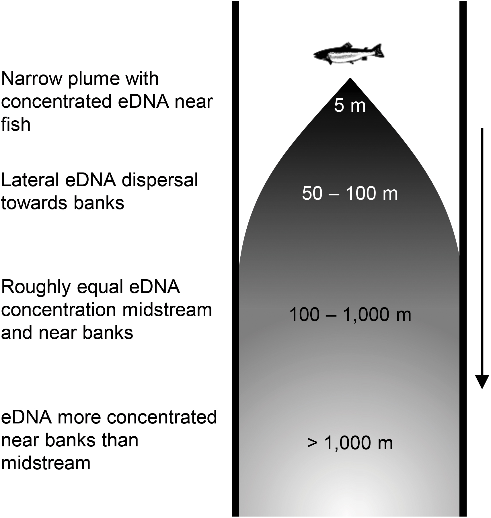
Figure 1. Hypothesized eDNA plume in rivers and streams. See section “Results” for explanation of distance estimates and plume phases.
Stream eDNA and Atlantic Salmon
Here we use Atlantic salmon in Bay of Fundy tributaries (New Brunswick, Canada) as a case study for examining spatial eDNA dynamics in streams. The abundance of Atlantic salmon has declined well below their conservation limits in the Bay of Fundy since the 1980s, with several stream-specific populations being extirpated from their native habitats (Jones et al., 2014; Fisheries and Oceans Canada, 2019). As they migrate back and forth between freshwater and marine environments to complete their life cycle, Atlantic salmon can be particularly vulnerable to a gauntlet of anthropogenic stressors along their migration corridor (Parrish et al., 1998; Cairns, 2001; Limburg and Waldman, 2009; Brown et al., 2013). As a result, fishery restrictions and recovery measures have been put in place to protect and recover these populations (Fisheries and Oceans Canada, 2019). Assessing their distribution and the habitat suitable for spawning, growth, and survival of juveniles in streams and rivers is thus essential to developing efficient protection and habitat restoration management strategies. Quantitative population size is also essential to evaluating the effectiveness of various recovery measures. However, current methods for assessing the distribution and abundance of Atlantic salmon in streams and rivers are time consuming, require considerable effort in the field, and risk inadvertent injury or mortality to salmon (Dolan and Miranda, 2004; Rummer and Bennett, 2005; Miranda and Kidwell, 2010). Spatial eDNA distribution models will lead to stronger salmon quantitative population estimates if we better understand how eDNA disperses and dilutes within the environment.
This project aims to develop a framework to assess quantitative population distribution in lotic ecosystems based on the spatial distribution of eDNA. First we evaluated spatial eDNA distributions and tested if the plume model is valid based on known quantities of salmon placed into sentinel cages in three salmon-free streams in Southwest New Brunswick. Second, we used the results from these sentinel cage experiments to build a model that uses eDNA dynamics to pinpoint and quantify upstream fish.
Materials and Methods
Salmon Experiment and eDNA Capture
We placed 3, 10, 30, or 63 Atlantic salmons in sentinel cages in three streams in Southwest New Brunswick, Canada that contain little to no salmon (Jones et al., 2014): Dennis (45°15′13.32″ N, 67°16′2.639″ W), Waweigh (45°14′57.206″ N, 67°7′57.9″ W) and Digdeguash (45°23′6.151″ N, 67°8′52.065″ W). Atlantic salmon has not been detected during intensive electrofishing surveys conducted in the Dennis Stream and Waweig River in recent years, while typically a few have been caught each year in the Digdeguash River since 2009 (Graham Chafe, Atlantic Salmon Federation, personal communication). All three streams are shallow with rock bottoms and detailed physical conditions of each stream are presented in Table 1. The experiments were conducted in June (Dennis and Waweig: 3, 10, and 30 fish; Digdeguash: 10 and 63 fish) and in October (Dennis: 10 and 30 fish; Digdeguash: 10 fish). Each deployment consisted of adding a low abundance of fish (e.g., three fish) to the cage and collecting water samples 24 h after. Following water collection, fish were added to the cage to a higher desired abundance and water was again collected after 24 h. The cage (size: 4′ × 4′ × 2′) was made of 1/2″ hardware mesh with edge PVC pipe for reinforcement and a 2′ × 2′ opening panel on top. The cage was fixed to the stream bottom by adding rocks. Leaves and debris were retained by a 1/2″ hardware mesh installed about 20 m upstream of the cage. For each deployment and fish abundance, water samples (1 L) were collected from downstream to upstream from the cage at 1,600, 800, 400, 200, 100, 50, 5 m and approximately 50 m upstream. Additionally, Dennis Stream and Digdeguash River were also surveyed at 6,000 and 7,000 m, respectively. At each sampling distance, water samples were collected at each bankside and mid-stream for each lateral transects; a single 1 L sample was taken at each location (i.e., for a total of three samples per distance). To mitigate potential contaminations, 1 L Nalgene® bottles were shaken with 10% bleach solution (Clorox Javex® 12, 10.3% sodium hypochlorite) three times followed by five times with distilled water. We rinsed the bottles with river water three times prior to collecting the 1 L water samples to wash away any remaining bleach residue. For all surveys, sampling commenced at the most downstream location and moved upstream to reduce disturbance of eDNA that might be present in the riverbed. We collected surface water by fully submerging the bottles right below the surface while facing upstream. Nitrile gloves were worn and replaced between sampling sites and field controls to reduce contamination risks.
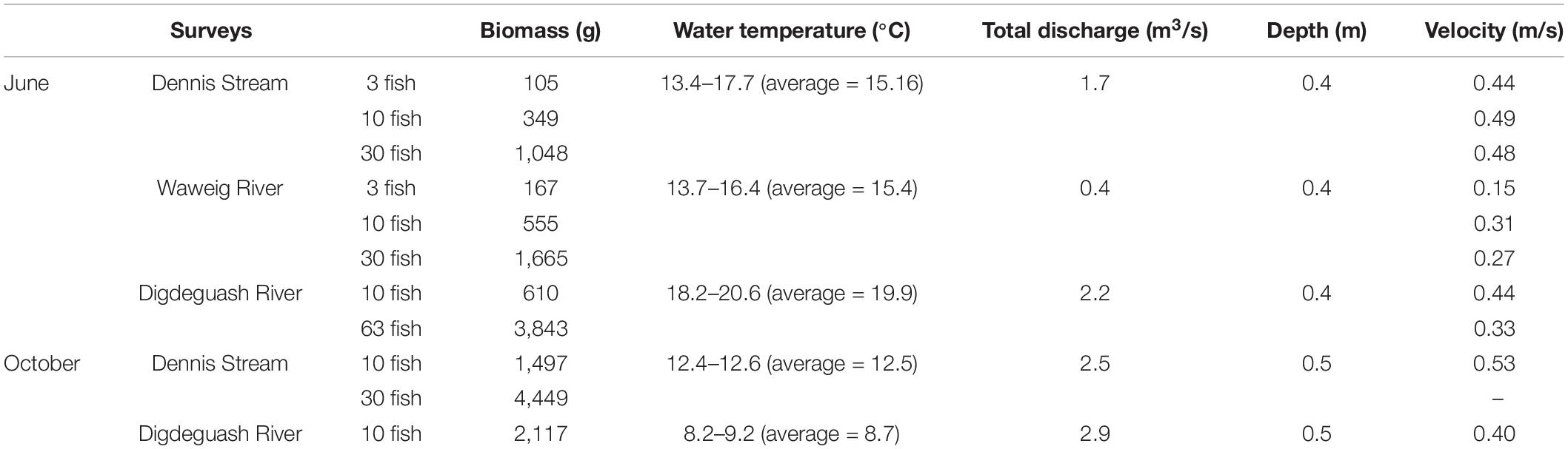
Table 1. Environmental conditions within each stream during the experiment periods.
Water samples were kept on ice, and then at 4°C until filtration, which was performed in a dedicated filtration laboratory within 24 h of collection. All filtrations were done with 47 mm diameter 0.8 μm Whatman nylon membrane filters (GE Healthcare, IL, United States). Field blanks (tap water) were brought in the field during water sample collection and processed alongside stream samples for each sampling event. Lab filtration blanks, DNA extraction blanks and qPCR negative controls were also included during the processing and testing of samples. Furthermore, all reusable equipment (e.g., mason jars, forceps, and vacuum flasks) was soaked in a 1% bleach solution (i.e., 1 in 10 dilution prepared from 10% commercial bleach) for a minimum of 1 h.
Molecular Analyses
Atlantic Salmon qPCR Assay Design and Optimization
Atlantic salmon DNA barcode sequences from local specimens as well as sequences found in NCBI1 and BOLD2 were aligned in Geneious (version 9.1.4) along with DNA sequences from close relatives and other species with high nucleotide similarity (≥85%) and/or a similar geographic range. Specific primers [COI_82F_Ss (5′-TGGCGCCCTTCTGGGA-3′) and COI_276R_Ss (5′-AAGGAGGGAGGGAGAAGTCAAAAA-3′)] and probe [COI_194P_Ss (FAM -- ATTAATTCCTCTTATAATCGGG -- MGB)] were designed in silico to amplify a 195 base pairs (bp) region of the mitochondrial cytochrome c oxidase subunit 1 (CO1). To ensure species-specificity, the assay was designed with a high number of nucleotide polymorphisms between the targeted species and closely related and sympatric species. Primer-BLAST3 was also used to ensure that primers were target-specific. The specificity of the qPCR assays was also tested in vitro using DNA from species that are closely related and/or potentially present in the studied environments : Salmo trutta, Salvelinus fontinalis, and Morone saxatilis. Serial genomic DNA dilutions were done to determine the efficiency [E = −1 + 10(–1/slope)] and calculate the theoretical limit of detection (LOD) and limit of quantification (LOQ). Three serial dilutions from 100 to 10–8 were prepared and each serial dilution was tested in duplicate for a total of six qPCR threshold cycle (Ct) values. The theoretical LOD and LOQ was determined according to Klymus et al. (2020) using the discrete detection threshold approach. Non-target DNA normalized to 5 ng/μL was used as a background when preparing the serial dilutions to assess the efficiency of the assays under conditions similar to its prescribed usage.
DNA Extraction and Species-Specific qPCR Testing
DNA extraction from filters was conducted using half of each filter with the MN NucleoSpin Tissue Kit (Macherey-Nagel, PA, United States) following a modified protocol (LeBlanc et al., 2020). The resulting DNA extracts were stored at −20°C and the second half of the filter was kept as a back-up.
qPCR testing was done with the species-specific Atlantic salmon qPCR assay using the 2× TaqMan Gene Expression Kit (Thermo Fisher Scientific, MA, United States). Briefly, 3 μL of template DNA, 480 nM of each primer, 200 nM of the probe, 1 μL of 1% BSA, as well as 12.5 μL of master mix were used in 25 μL reactions. All qPCR tests were done in triplicate on a StepOnePlus qPCR platform (Thermo Fisher Scientific, MA, United States) using the following cycling parameters: initial hold at 50°C for 2 min, 95°C for 10 min, followed by 40 cycles at 95°C for 30 s, 60°C for 30 s and 72°C for 30 s, with fluorescence reading at the end of each elongation cycle. An exception to this was the samples from October, for which 50 qPCR cycles were used.
Sample Quality Control and Confirmation
To evaluate if PCR inhibitors were present in environmental samples, which could lead to potential false negative results, all samples (including blank controls) were spiked with an exogenous internal positive control (IPC) (linearized DNA plasmid containing a DNA sequence not found in the targeted environments) and tested using a qPCR assay specific to that IPC. Inhibition was considered present if a difference of more than 2 between the qPCR Ct of environmental samples and field blanks was observed. The IPC qPCR assay was done using the same parameters and reagents used for the species-specific Atlantic salmon qPCR assay.
To confirm the specificity of field results, sanger sequencing was performed on a subset of samples (6%). Briefly, PCR was performed using the optimized species-specific qPCR assay and the AmpliTaq Gold 360 PCR Master Mix (Thermo Fisher Scientific, MA, United States). PCR products were visualized on a 1.5% agarose gel followed by PCR product cleanup using ExoSAP-IT (Affymetrix, CA, United States) prior to being sent for Sanger sequencing at the Centre d’expertise et de services Génome Québec (Montréal, QC, Canada).
The Atlantic salmon qPCR assay gave an efficiency of 95.9% and a theoretical LOD and LOQ of 0.36 pg (24 pg/L) and 2 pg (133 pg/L) of gDNA, respectively. The R2 value of the assay was 0.992 and eDNA concentrations (pg/L) were calculated from the equation: −3.4243[log(x)] + 24.475. Sanger sequencing on a subset of samples (6%), including some in October with Ct values >40 confirmed the assay as being specific to Atlantic salmon, with a few exceptions (mostly Ct > 44) which gave non-specific amplification; Ct values >40 have been kept to ensure capturing the full qualitative eDNA spatial distribution assessment.
Analyses
We conducted all analyses using R version 4.0.2 (R Core Team, 2020).
Data Availability
All data used in this study are available as Supplementary Material.
Exploring eDNA Spatial Distribution and Variation
First, we explored and described the spatial pattern of eDNA downstream of fish by examining the lateral and longitudinal distribution of eDNA. Second, we examined the effect of the water velocity and number of fish on spatial eDNA distribution and concentration. Finally, we examined the variability of eDNA detection and quantities across and within the three different streams.
Modeling eDNA Spatial Distribution and Variation
We built a model that reflected a combination of patterns in our data (Figure 2), trends from published studies, and first principle ecological assumptions, namely:
1. eDNA is more abundant when more fish are present (Pilliod et al., 2013; Doi et al., 2017; Wood et al., 2020)
2. eDNA decays or is lost as it moves downstream (Jerde et al., 2016; Wilcox et al., 2016; Laporte et al., 2020; Wood et al., 2020)
3. eDNA is less abundant when velocity is high (i.e., it is dissolved in a greater volume of water; Pilliod et al., 2014; Jane et al., 2015; Pont et al., 2018)
4. eDNA is initially entrained in the main flow of the stream, but disperses outward over time and distance toward the banks (hypothesized in Wood et al., 2020).
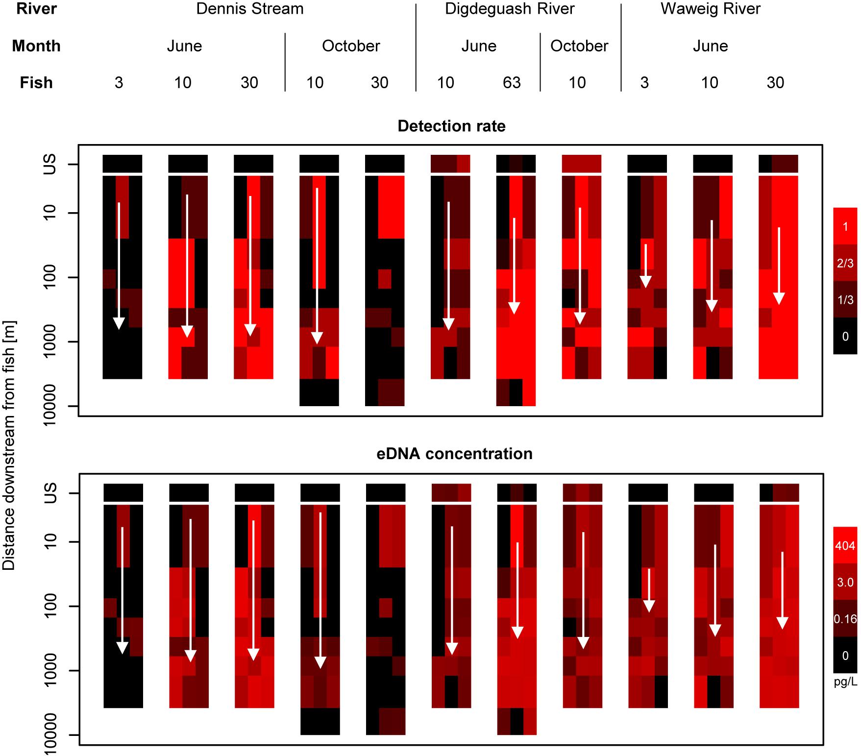
Figure 2. Salmon eDNA detection rates and quantities for bankside and midstream samples in three New Brunswick streams. White arrows indicate average stream velocity, which ranged from 0.15 to 0.53 m/s. Velocity data was not available for the 30 fish treatment in Dennis Stream in October. Detection rate is defined as the number of qPCR replicates where salmon DNA was detected. US, upstream control samples (see section “Materials and Methods”).
We tested these patterns and assumptions using likelihood ratio tests and relative likelihood (see below).
We modeled eDNA concentrations as an initial pulse in the center of the stream at the fish cage, with the pulse amount dependent on the number of fish. To account for lateral movement of eDNA within the stream (i.e., expansion of the “plume” perpendicular to the direction of water flow, Figure 1), we allowed the proportion of eDNA that was found at the banks to increase from 0 at the fish cage to a fixed (equilibrium) proportion moving downstream from fish. eDNA also was allowed to decay at midstream- and bankside-specific rates. eDNA detection was treated as a logistic function of predicted eDNA concentration. The following six equations represent sequential steps in one model that maximized the probability of obtaining our eDNA detection and quantity data (i.e., a maximum-likelihood model).
For the first step of the model, we modeled the proportion of eDNA found in the two bankside samples [PB(x)]. We assumed lateral dispersal (square-root) dynamics (Wetzel, 2001), with an asymptote at a given proportion (Pmax):
Pmax is the maximum proportion of eDNA found at the banks; γ is a lateral dispersal rate coefficient. For example, if Pmax = 0.4, then 40% of eDNA will be found in the bankside samples (rather than the midstream samples) far downstream from fish.
For the second step of the model, we modeled the total amount of eDNA [Q(x)] across two bankside samples and one midstream sample at downstream distance x, incorporating midstream and bankside eDNA loss rates (rm and rb, respectively), number of fish (F), and velocity (V). Midstream- and bankside-specific decay rates were weighted by the proportion of eDNA found at each [PB(x); Eq. 1] and followed exponential decay over distance (x). eDNA quantities were modeled as proportional to the number of upstream fish (F), and inversely proportional to velocity (V):
β0 is a stream-specific coefficient; F = the number of fish; PB(x) = proportion of eDNA in bankside samples (Eq. 1); rb and rm = eDNA decay rates at the banks and midstream, respectively; x = distance downstream; V = velocity; and q is a velocity scaling coefficient. We modeled β0 specifically for each stream to examine the variation in β0 for later analyses (see below).
For the third step of the model, we separated the quantity of eDNA found at a given distance [Q(x)] into its midstream [M(x)] and bankside components [B(x)] according to the proportion of eDNA expected at the midstream and banks [PB(x); Eq. 1]:
For the fourth step of the model, we calculated eDNA detection rates [RM(x) and RB(x) for midstream and bankside samples, respectively] from eDNA quantities. We assumed that eDNA detection was logistically related to eDNA quantity (Klymus et al., 2020), i.e., low quantities of eDNA led to low detection rates and large quantities of eDNA led to high detection rates:
α0 and α1 are rate and shape parameters, respectively, for the detection rate ∼ eDNA quantity relationship.
Finally, we calculated the likelihood of obtaining our eDNA detection and quantity data given the above model. We then optimized the model, picking the set of parameters that maximized the likelihood (i.e., minimized the negative log likelihood) using the mle function in the stats4 package, included in base R (R Core Team, 2020).
Model Testing – Parameters
We statistically tested the earlier described patterns and assumptions underlying the model. We tested the significance of several terms of interest (velocity, eDNA decay, inter-stream variation, and month-to-month variation) within the models using Type II likelihood ratio tests. We also tested the significance and precision of the eDNA quantity-detection rate relationship (i.e., Eqs 5 and 6) using a likelihood ratio test and a receiver operating curve (ROC).
Model Testing – Plume
To test for the presence of an eDNA plume (i.e., lateral diffusion of eDNA moving downstream from fish), we compared our model to several alternative models without lateral diffusion. These models are summarized in Supplementary Table 1. All alternative models have a fixed proportion of midstream versus bankside eDNA over all downstream distances from fish. The first alternative model assumes that eDNA is lost at a constant rate as it moves downstream from fish. The second assumes a lag period during which eDNA becomes easier to detect farther from fish, then is lost at a constant rate as it moves further downstream. The third assumes no changes in eDNA concentration moving downstream from fish.
As the four above models were not nested versions of each-other, we could not conduct likelihood ratio tests (Burnham and Anderson, 2003). Instead, we compared models using relative likelihood (Burnham and Anderson, 2004). We also calculated R2 for all models for both our eDNA detection and quantity data. As we only sampled downstream >1,600 m for a small set of stream/fish/date combinations, we repeated the above analyses with only data for distances ≤1,600 m to remove the potential for bias.
Model Testing – Bankside eDNA Accumulation
We also examined the asymptotic proportion of eDNA found in the bankside samples far downstream from fish (Pmax), as this parameter has important implications for accumulation or loss of eDNA near stream banks. We refit our model with Pmax fixed at the range of values from 0 to 1 and examined the model AIC. Again, as we only sampled downstream >1,600 m for a small set of stream/fish/date combinations, we repeated the above analyses with only data for distances ≤1,600 m to remove the potential for bias.
Optimal eDNA Sampling
We calculated detection power for two management scenarios: sampling downstream from a target reach (i.e., known or hypothesized fish location), and uniform sampling to detect fish in an unknown location. Significant variation exists across streams in eDNA detectability, even for the same number of fish and same volume of water (see section “Results”), likely due to the stochastic dispersion from stream-specific hydrodynamics and differences in stream morphology, as well as water chemistry (Dejean et al., 2011; Barnes et al., 2014; Deiner and Altermatt, 2014; Jerde et al., 2016; Shogren et al., 2016, 2018; Klymus et al., 2020). This variation is reflected in the stream- and date-specific β0 parameter in Eq. 1. Thus, power analyses for eDNA detection must be sensitive to this variation, and generate predictions that work for most streams, rather than just the average stream. We used the distribution of the stream- and date-specific β0 parameter to generate a “low detection” β0 value corresponding to 5% quantile for the β0 parameter distribution using the quantile function in R. As 95% of streams are expected to have higher detection than reflected in this “low detection” β0 value, we expect the below sampling analyses to be a conservative estimate for nearly all streams similar in character to our study systems.
Sampling downstream from a target reach
We examined the power to detect fish in a single reach, i.e., where fish presence was known, hypothesized, or of potential management concern. We calculated the number of samples required for positive detection (S) for different numbers of fish (3, 10, and 30), downstream distance (1–10 km), velocity (0.15, 0.35, and 0.55 m/s), and bankside/midstream sampling:
R is detection rate (Eqs 5 and 6) and A is desired power (i.e., A = 0.05 for 95% chance of detection). We used model parameter values from the maximum likelihood model fitting described above, with the exception of β0, for which we used the “low detection” value calculated above.
Constant-interval sampling to detect fish in an unknown location
We also tested the power of constant-interval sampling to detect fish presence anywhere in a stream, when potential fish location is unknown. This is the case for sampling studies looking to broadly describe species’ distributions, in which simple presence/absence is sought in numerous streams. In this case, constant-interval sampling over the course of a stream is one method to determine whether fish are present (Wood et al., 2020). Following Wood et al. (2020), we simulated varying numbers of fish (1, 3, and 10) at a single, random location in a 100 km stream with different water velocities (0.15, 0.35, and 0.55 m/s). We then assumed a constant-interval (10–2,000 m), midstream sampling effort with three technical replicates. We examined fish detection rate with 10 replicate simulations per each fish, velocity, and sampling interval combination.
Results
Environmental DNA concentrations downstream from fish were highly variable across and within streams, dates, and numbers of fish, ranging from no detections to 731 pg/L. The mean eDNA concentration for all samples with a positive detection was 25.6 pg/L and the lowest concentration detected was 0.01 pg/L. eDNA was detected in 56% of our samples, including 22% of samples taken 6 or 7 km downstream from caged salmon.
Similar to our expectation, a low concentration of eDNA was detected upstream of the cage deployment site in the Digdeguash (30.6% positive detection in the upstream samples, mean: 3.29 pg/L) and Waweig Rivers (7.4% positive detection in the upstream samples, mean: 3.78 pg/L). The various field and laboratory filtration blanks, as well as DNA extraction and qPCR negative controls included throughout this work showed minimal potential cross-contaminations, with only 1 out of 15 field blank (eDNA concentration = 4.19 pg/L) and 1 out of 28 DNA extraction blank (eDNA concentration = 2.1 pg/L) positive for salmon DNA.
eDNA Spatial Distribution and Variation
Environmental DNA concentrations and detections were highest midstream and lowest bankside shortly downstream from fish (Figures 2, 3). Up to roughly 100 m downstream from fish, eDNA quantities and detection rates remained higher midstream, but became increasingly abundant bankside (Figures 2–4). Between 100 and 1,000 m, we observed roughly equal eDNA detection rates and quantities in midstream and bankside samples, followed by higher eDNA detection rates and quantities at banksides located >>1,000 m from fish (Figures 2, 3). There was, however, significant variation within streams that added noise to—and sometimes masked—these general patterns. eDNA concentration variation was highest midstream closest to fish (5 m downstream), and lowest bankside closest to fish (Figure 5)—both for untransformed variation and variation of ln-transformed data, which removes right skew and assumes variance is proportional to the mean. Thus, the eDNA spatial distribution exhibited unique midstream and bankside patterns with increasing downstream distance from fish. Midstream, eDNA had initially high abundances, with relatively constant loss moving downstream (Figure 6). On the other hand, bankside eDNA was nearly undetectable close to the fish, but gradually rose in abundance, then fell again with increasing downstream distance from fish (Figure 6 and Supplementary Figure 1). Thus, eDNA data showed a steady dispersal of eDNA from the midstream toward the banks over distance (Figures 1, 3 and Table 2), which resulted in the eventual “buildup” of eDNA on the banks >1,000 m downstream from the fish (Figures 2, 3).
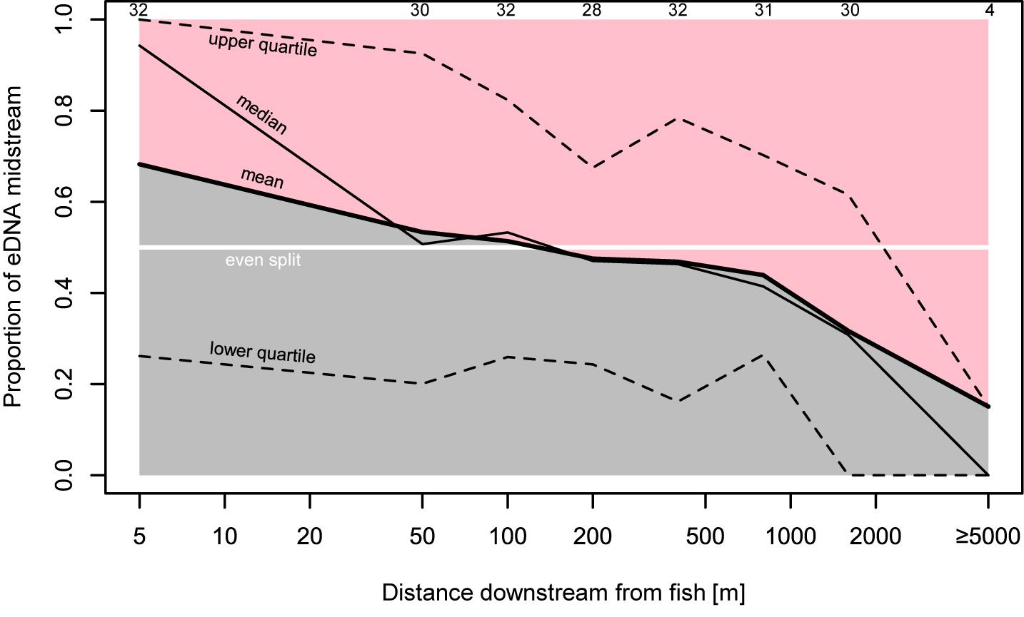
Figure 3. Proportion of bankside versus midstream eDNA. Proportions here are calculated as the midstream eDNA quantity over the midstream eDNA quantity plus the average of both bankside quantities. All sampling transects in which at least one sample had positive detection are included here. Top numbers indicate number of transects included in proportion estimate.
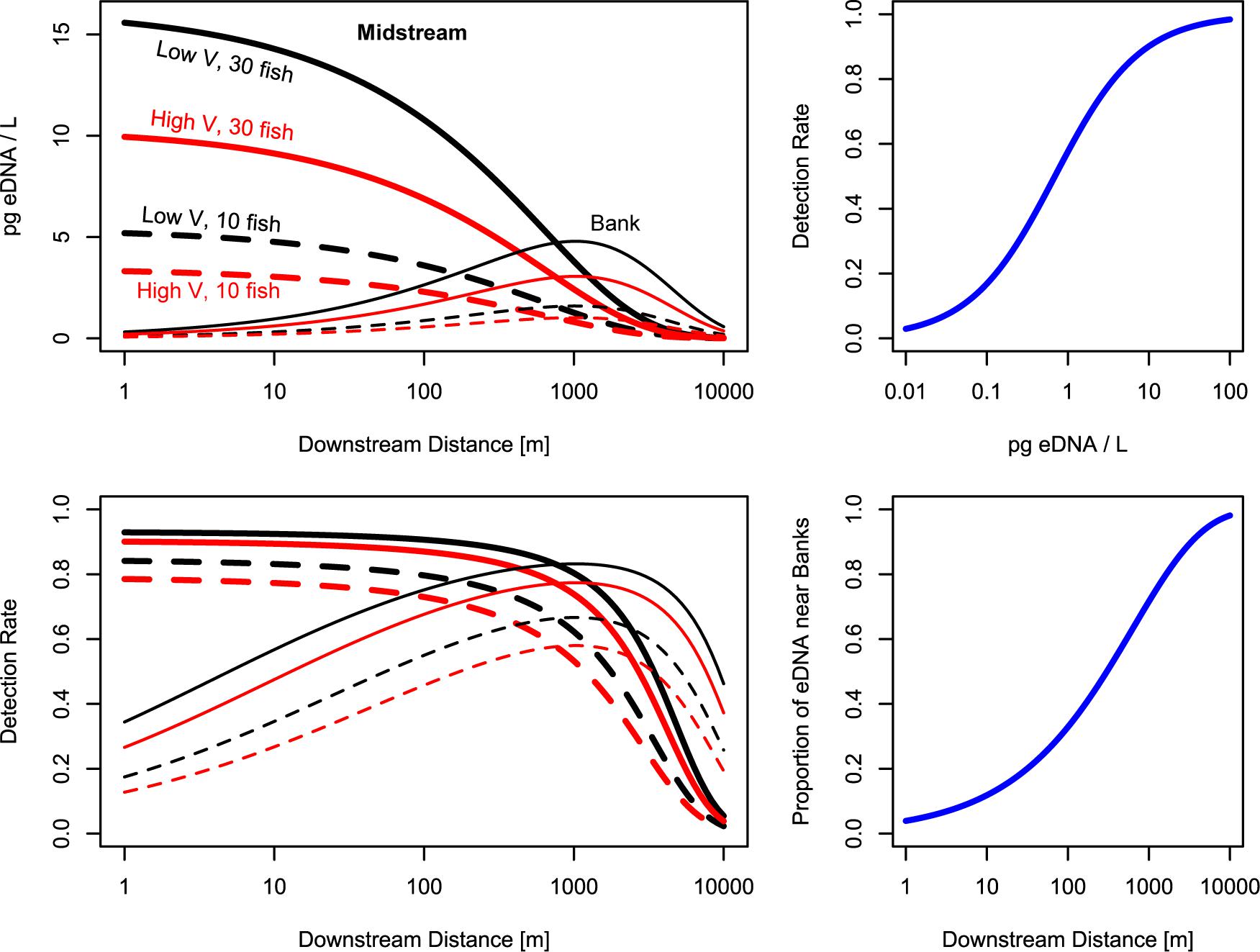
Figure 4. Modeled salmon eDNA quantities and detection rates downstream from fish. Top left: eDNA is most abundant near the fish, then disperses to the banks, where eDNA is most abundant roughly 1,000 m downstream from the fish. Values shown are predicted values for an average stream. Top right: after roughly 1,000 m, more eDNA can be found in bankside samples than midstream samples. Bottom left: Midstream samples have higher detection rates near the fish, while bankside samples have higher detection rates roughly 1,000 m downstream from the fish. Bottom right: eDNA detection rates are greater than 50% when predicted eDNA concentrations are >1 pg/L; eDNA detection rates are roughly 90% when predicted eDNA concentrations are >10 pg/L.
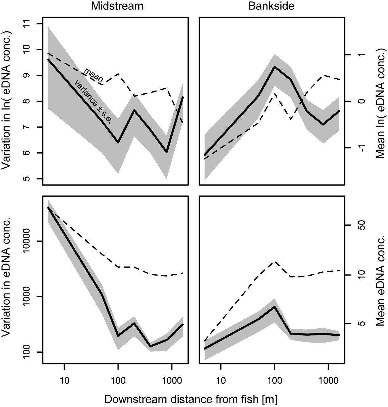
Figure 5. Variation and mean eDNA abundance. Distance-specific variances for midstream and banks samples shown, pooled across all streams, dates, and fish abundances for each distance. Distances >1,600 m, which were not sampled for all streams, were excluded from this figure. The variance of ln-transformed data reduces the potential effect of variance scaling with the mean [i.e., ln(με) becomes ln(μ) + ln(ε)] and is less sensitive to outliers.
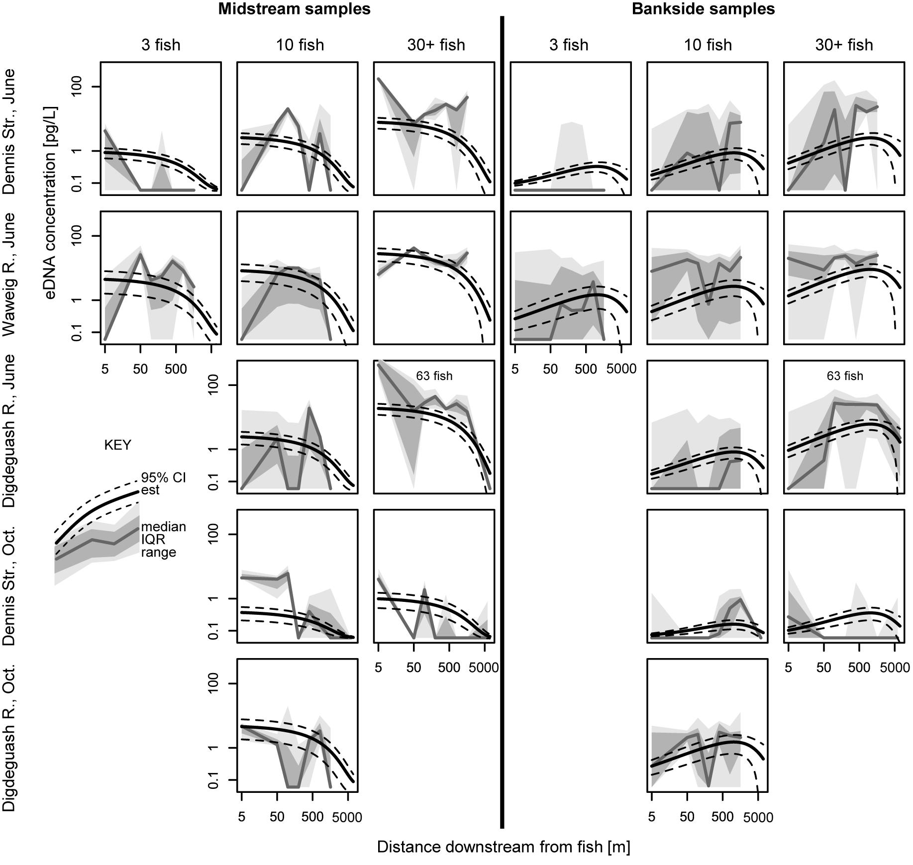
Figure 6. eDNA concentration versus downstream distance from fish, separated for midstream and bankside samples. Data distributions, model estimates, and model estimates confidence intervals (CI) are shown. IQR, inter quartile range. For analogous eDNA detection rate data, see Supplementary Figure 1.
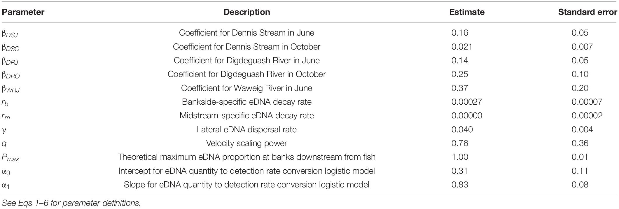
Table 2. Parameter estimates and standard errors for eDNA detection rate and concentration models.
Model Testing – Parameters
There was significant stream-level variation and temporal variation in eDNA detection and quantity (i.e., variation in β0) that was not related to velocity or number of fish (Table 3). eDNA detection rates and quantities were significantly lower at higher velocity (Table 3). Our model showed significant eDNA decay or loss as it moved downstream; this loss occurred more rapidly at the banks according to our model, though this difference was not statistically significant (Table 3). Finally, our model showed a significant relationship between eDNA concentration and detection rate, with a relatively strong ability to discriminate between positive and failed detections (Supplementary Figure 2).
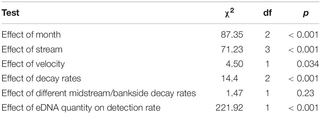
Table 3. Likelihood ratio tests for model parameters.
Model Testing – Plume
Our model strongly outperformed the three alternative models—all of which assumed no lateral dispersal of eDNA (i.e., no plume)—in both relative likelihood and R2 (Table 4). The same pattern was apparent even when sampling distances >1,600 m were excluded from our analyses (Supplementary Table 2). Thus, lateral dispersal, rather than differential midstream/bankside eDNA decay rates, appeared to drive the differences in midstream and bankside eDNA dynamics in our model.
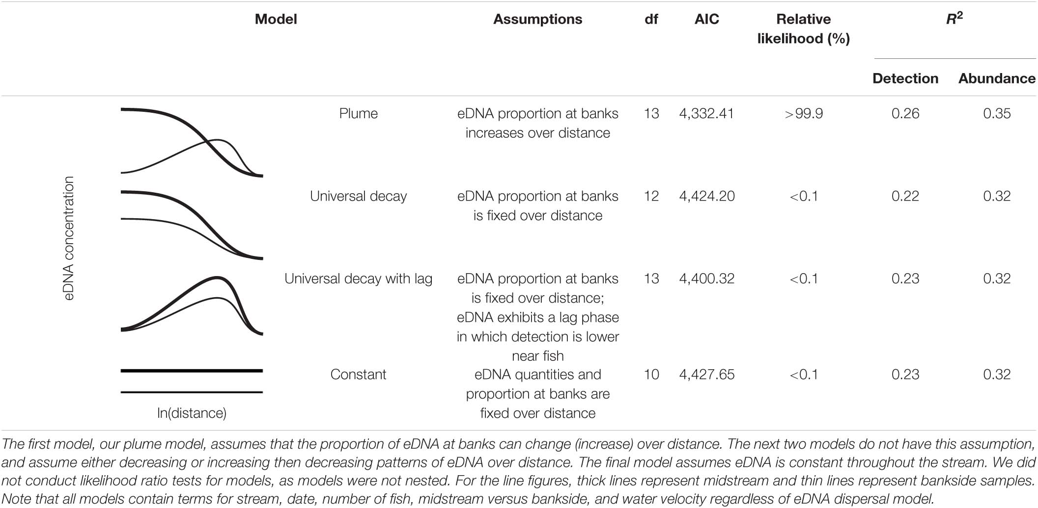
Table 4. Comparison of four eDNA dispersal models.
Model Testing – Bankside eDNA Accumulation
The optimal (in terms of AIC) value for Pmax—the asymptotic proportion of eDNA found in bankside samples downstream from fish—was approximately 1.00 when all data were included and 0.95 when only distances ≤1,600 were included in our analyses (Supplementary Figure 3). Decreasing Pmax to 0.67—the value expected if eDNA was evenly dispersed across one midstream and two bankside samples far downstream from fish—increased the model AIC >> 5 in both cases.
Optimal eDNA Sampling
We found that optimal sampling for eDNA is near the source for midstream samples, and roughly between 100 and 1,000 m downstream for bankside samples (Supplementary Figure 4). However, our midstream results are slightly misleading without context, as our midstream sampling was conducted with the knowledge that our salmon were in the very middle of the stream. In reality, midstream sampling may have less optimal results shortly downstream from fish when the lateral positioning of the fish is not known. The optimal sampling distance that gave relatively high detection rates for both midstream and bankside sampling was roughly between 100 and 1,000 m downstream from fish.
Based on our constant-interval eDNA sampling power analysis, sampling midstream every 100 m (with three replicates) was sufficient to detect a single fish (>95% power) under high-velocity conditions in a low-detection (5% quantile β0) scenario (Supplementary Figure 5). At low velocity, this sampling distance increases to about 400 m. With 10 fish present, sufficient sample spacing increases to 500 to > 1,000 m, depending on velocity (Supplementary Figure 5).
Discussion
Consistent with other studies, our results indicate that eDNA is a reliable indirect approach for determining organism presence in streams. As expected, concentrations of eDNA increased predictably with the number of upstream fish (Figures 2, 6). However, estimating fish distribution and abundance precisely require accounting for distance and flow. Our results demonstrate that a better understanding of spatial patterns of eDNA concentration, variation, and distribution is important for optimizing eDNA detection and essential to assessing quantitative population distribution in lotic environments. We examined the spatial dynamics of eDNA as it moves downstream from fish and found evidence of an eDNA plume—eDNA exhibiting a pattern initially concentrated in the midstream but widening as it travels downstream from fish (Figure 1). These dynamics were clear even despite a low level of upstream eDNA contamination in a few instances (see section “Results”). The detection rate and quantity of eDNA varied widely across rivers and sampling periods, but varied predictably with the number of upstream fish and velocity. Below, we discuss how physical factors can be gathered to predict quantitative population distribution in a single and multiple inhabited reaches based on the eDNA plume.
Characterizing the eDNA Plume
Results support that eDNA spreads from fish in the form of a plume beginning as concentrated large particles (e.g., tissue fragments and cells) close to the fish (Wilcox et al., 2015). Due to its state, eDNA concentrations near the source are highly variable with high upper concentration limits in the midstream (Figures 2, 5). eDNA is then more evenly dispersed over distance due to the “breakout phase” processes wherein particle fragmentation and mixing result in smaller, more evenly distributed particles (Figure 3). In the breakout phase, eDNA becomes more equally abundant in midstream and bankside samples. Beyond this breakout zone, our results support that there is a more steady decrease in detection due to DNA degradation, dilution, and settlement (Barnes et al., 2014; Jerde et al., 2016; Shogren et al., 2017), but again this differs between midstream and bankside regions. Past the point of roughly equal eDNA in the midstream and bankside regions, eDNA persists at higher concentrations near the banks while eDNA drops off more in the midstream (Figures 2, 3).
Similar to fine particles, eDNA tends to accumulate in stream margins where the velocity is low. The shape of the plume process is likely to be driven by the hydrological water-bank interface. Based on fluid dynamic theory, stream velocity is greatest in the midstream near the surface and is slowest along the stream bed and banks due to friction. Faster flow tends to be turbulent, while slower flow tends to be laminar. Turbulent flow is more effective than laminar flow at keeping particles in suspension. Studies report a high degree of fine-particle retention within the streambed and banks (Skalak and Pizzuto, 2010 and Harvey et al., 2012). Banks can thus act as “sponges,” catching and accumulating eDNA on sediments, complex debris, and in eddies while midstream eDNA is continually flushed out of the system or stochastically dispersed laterally. Other work has demonstrated net movement of organic matter out of the water column and into superficial sediments (Minshall et al., 2000), leading to higher eDNA concentrations in and near sediments (Turner et al., 2015). Thus, we hypothesize that bankside samples sufficiently downstream from fish have higher concentration than their respective midstream samples due to proximity to eDNA-rich sediments and eddies. Particularly, these observations suggest that eDNA does not behave strictly as “wash load” and instead depict the combination of downstream transport and transient retention influenced by stream geomorphology (Drummond et al., 2017; Phillips et al., 2019).
Overall, we observed the predictable pattern of decreasing eDNA concentration and detection rate with increasing velocity—a proxy for flow rate (Figure 4 and Table 3). Similar to results from particle models (Andruszkiewicz et al., 2019), increasing the volume into which eDNA is diluted is at least partially responsible for this pattern. However, it remains to be seen whether increasing velocity—and thereby flow rate—leads to a greater transport distance for eDNA, shifting or stretching our eDNA detection curve longitudinally by modifying rb, rm, γ, or pmax (Pilliod et al., 2014; Pont et al., 2018). In midstream nearby the source (50–240 m), Jane et al. (2015) observed that, despite high variation between ecosystems, eDNA abundance was highest close to the source and quickly trailed off over distance at the lowest flows, whereas eDNA was relatively low both near and far from the source at the highest flows. Here, the relatively small number of distance sampling points, combined with our relatively high detection rates at 6 and 7 km downstream from fish, make this question better addressed by future studies.
Optimal Sampling
Determining the optimal eDNA sampling strategy depends on correctly and accurately quantifying the eDNA plume. When water samples are collected only a few meters downstream from the target organism, more replicates, water volume, or pooling water samples might be needed to overcome the high variation seen in samples near the target organisms (see section “eDNA Spatial Distribution and Variation”; also see Wood et al., 2020). However, as the lateral positioning of the target organism is generally unknown, many samples taken a few meters downstream from a target organism or reach are likely to miss the plume and have low eDNA concentrations or detection rates (as in the bankside samples, Figures 2, 5). Therefore, while sampling in the plume immediately downstream from the fish would technically yield the highest quantity of eDNA, chances of successfully sampling in the plume close to the fish are lower. In the systems surveyed in this study, the highest eDNA detection probabilities and mean concentrations across all lateral sampling positions occurred between 100 and 1,000 m downstream of the source. Importantly, we do not recommend single-bankside eDNA sampling, due to the tendency of one bankside to be consistently biased compared to the other (see Figure 2). Instead, we recommend midstream sampling or combined sampling of both banks. The importance of field replicates is crucial in all locations (see Figure 6).
For studies that simply seek system-wide detection of rare taxa, even-interval eDNA sampling is a potential cost- and labor-saving method. Our simulations indicated that sampling every 100 m gives a 95% chance of detecting even a single fish in high velocity (0.55 m/s) conditions in nearly all streams of similar character to the study streams. Increasing the number of fish or decreasing velocity allows for significantly less sampling—to about 400 m for our low velocity (0.15) scenario or about 600 m for 10 fish (see Supplementary Figure 4). These estimates are likely conservative estimates, as our experiments—despite sampling to 7,000 m in some streams—were unable to find a downstream LOD. Thus, these estimates are slightly influenced by extrapolation from our model, which assumed that midstream eDNA detection was virtually impossible after 10,000 m.
Quantitative Population Distribution Assessment Using eDNA
Excitingly, the predictable patterns of midstream versus bankside eDNA transport should in principle allow one to estimate upstream fish distance and number using midstream and bankside water sampling, e.g., presented in Figure 7. In other words, eDNA heterogeneity across a stream channel can facilitate distributional assessment, the third operational goal for eDNA that has lagged detection and abundance quantification. Models can be solved for the proportion of eDNA in midstream samples and the total amount of eDNA in midstream and bankside samples to predict location and number of upstream fish. Box 1 presents two different scenarios: a single inhabited upstream reach, and numerous inhabited upstream reaches. The first scenario is relatively straightforward, as it simply requires solving of our models here for different variables. The second scenario is more realistic, but requires a layer of simulation and model fitting. Both scenarios assume fish are in midstream and in a similar type of stream as those selected in our study. We encourage stimulating datasets to calibrate and improve the performance of this predictive population model. Estimates of fish location can be confirmed with the expected spikes in midstream eDNA variation (Figure 5).
BOX 1. A framework to infer a population estimate model based on the spatial eDNA concentration in lotic environments.
Single inhabited reach case
Assuming two bankside samples (B1 and B2) and one midstream sample (M), the proportion of eDNA at the bankside is obtained as:
Then we can solve Eq. 2 (see section “Materials and Methods”) for distance, x, assuming we have already estimated the parameters Pmax and γ, the maximum eDNA proportion at banks and the lateral eDNA transport diffusion rate, respectively:
Now that we have distance, x, we can solve Eq. 1 for F, assuming we have already estimated the parameters q, β0, rb, and rm, the velocity scaling power, stream-specific coefficient, and bankside- and midstream-specific decay rates, respectively:
Now we have successfully calculated estimates of F and x for the studied fish size—the number of fish and the distance upstream from sampling. A single stream location for such sampling is apt to result in considerable positional and abundance estimation error. However, this can be improved upon by averaging or model fitting the respective estimates of F and x for multiple cross-stream sampling locations would permit more precise, consensus estimates of where and how many fish are present.
Multiple inhabited reaches case
When there are multiple potential inhabited reaches, each eDNA sample becomes an unequally-weighted picture of all fish upstream of the sampling site. The simulation of a given number of reaches i, each with its own number of fish Fi can then be calculated from the expected amount of eDNA for each sample, j, using Eq. 1 for Q:
We can then estimate the values for xi, Fi, and a standard deviation parameter s that maximize the likelihood, L (minimize the negative log likelihood) of generating our sample data, i.e., by maximum-likelihood model fitting:
Where pN is the probability density estimate of a normal distribution.
The AIC is then obtained from:
If we plot AIC versus i (the number of simulated reaches), an upside-down hump-shaped curve is obtained, as adding additional values for xi and Fi (reach distance upstream and number of fish in that reach, respectively) gives us diminishing marginal returns that are penalized when calculating AIC (via the 4i term). Thus, the maximum-likelihood estimates for xi and Fi associated with the minimum AIC are the most reliable estimates for fish locations and abundances. This is a quantitative population distribution assessment (Figure 7). Note that numerous eDNA samples will need to be taken at various longitudinal locations within a stream to generate the necessary power to fit multiple xi and Fi terms with any accuracy.
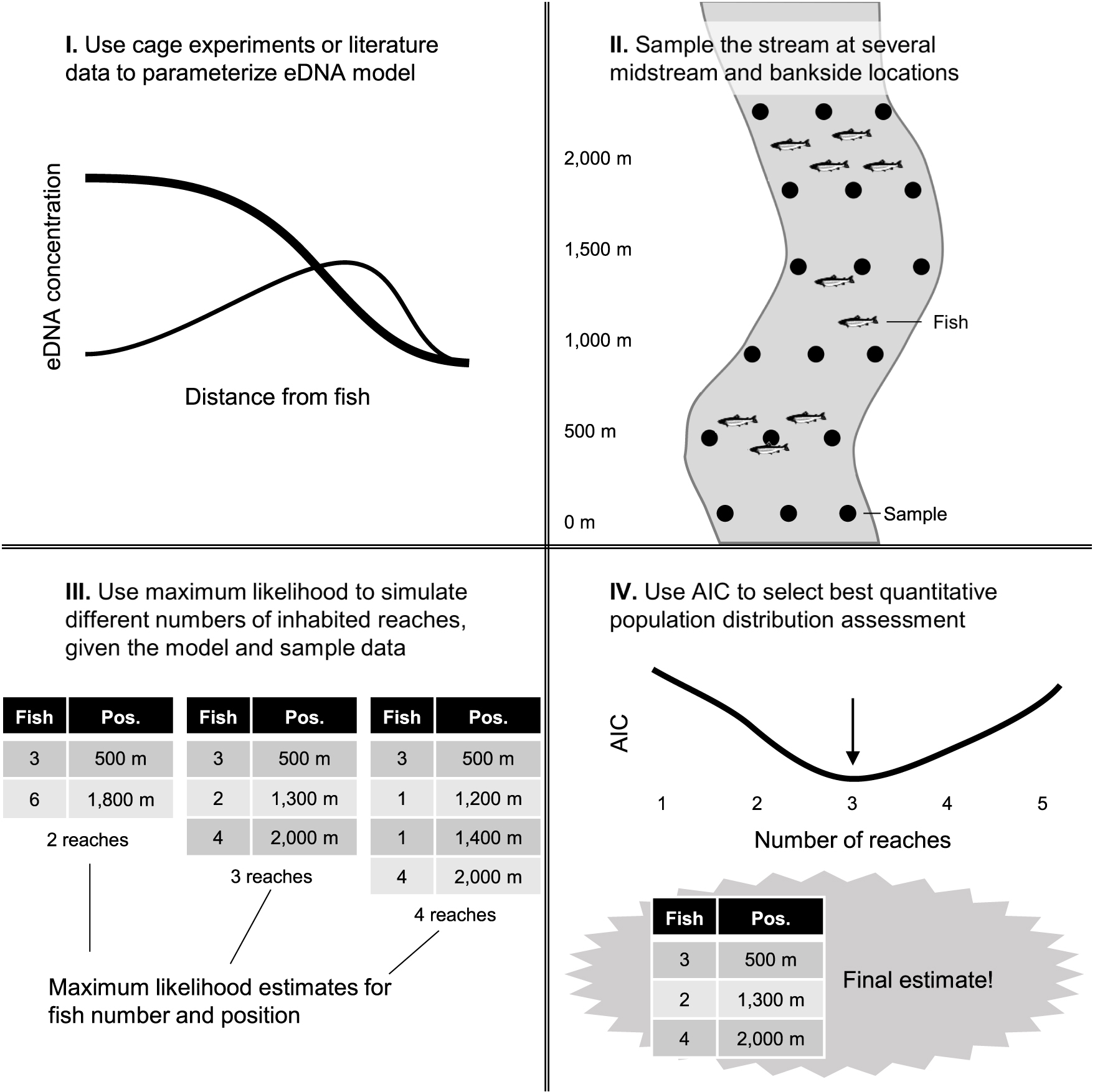
Figure 7. Workflow for eDNA-based quantitative population distribution assessment in streams. Once a sufficient model of eDNA dynamics is constructed for a particular stream or stream type, sampling and maximum likelihood simulations can give estimates of fish numbers and locations.
Next Steps—Environmental Covariates
The predictive models developed here are based on a large range of fish abundances and environmental conditions, at least within this study system of small shallow streams with rocky bottoms. However, here models assume that fish size is relatively constant and much variation in eDNA concentrations within and across streams and seasons remains—despite the general lack of PCR inhibition in our samples (Figure 6). This variation reflects complex interactions between the environment, organisms, and eDNA. More studies are needed to determine the probability that eDNA particles will go back to the mid-channel when the lateral positioning of the fish is not known, in order to decide where best to sample, i.e., mid-stream versus bank sides. There is an extensively growing literature about the effect of environmental conditions on eDNA dynamics, but a significant amount of effort is still needed to understand and account for these complex interactions. Quantifying the environmental parameters altering the eDNA breakout phase and the spatio-temporal variation of the eDNA plume should further improve the population predictive models included in this article—in particular by removing the need for a stream-specific parameter (β0, Eq. 1) in our models, instead replacing it with a universal parameter and environmental covariates. To efficiently extrapolate our predictive model to all types of Atlantic salmon habitats, it will also be important to test and calibrate a tridimensional model in larger rivers where sinking, settlement, and resuspension processes can have a significant effect on eDNA. Ideally, a next step in integrating eDNA into salmon management will be a salmon population distribution model based on the combined effect of eDNA dilution rate, persistence, life stage parameters, and environmental covariates. Such a model will be crucial to expand eDNA monitoring efforts to new streams.
Conclusion
Despite significant room for model development, eDNA is a powerful and growing tool for the conservation of riverine fish species. An essential component to using river eDNA to enumerate upstream stocks is an understanding of eDNA plume dynamics and its variation. As we have shown, plume dynamics may be leveraged to develop quantitative population distribution assessments in lotic environments that feed into management decision making. This spatial capacity would be a significant refinement to eDNA sampling which is currently largely used for detection and coarse abundance estimation. Further inclusion of source-specific eDNA release rates (e.g., fish life stages and metabolism) and environmental covariates will hopefully reduce much of the unexplained variability in eDNA data and generate eDNA models that are robust across study systems and management needs.
Data Availability Statement
The original contributions presented in the study are included in the article/Supplementary Material, further inquiries can be directed to the corresponding author/s.
Ethics Statement
The “animal study was reviewed and approved by the Animal Use Protocol, Fisheries and Oceans Canada, following values and standards promoted by the Canadian Council on Animal Care”.
Author Contributions
ALR, MT, NG, FL, and MK conceived the study and contributed the resources. The sampling design has been developed in close consultation between all co-authors. CB, ALR, NG, and FL contributed to field coordination/data collection. FL and NG developed and led the laboratory analyses. ZW analyzed the data. ZW and ALR wrote the manuscript, while FL, NG, MT, and MK helped to draft and improve the manuscript. All authors edited the manuscript and approved the final version.
Funding
This work was supported by the Strategic Program for Ecosystem-Based Research and Advice (SPERA) and Genomics Research and Development Initiative Phase VII (GRDI) from Fisheries and Oceans Canada (DFO), the Maine Agricultural and Experiment Station, the University of Maine Janet Waldron Doctoral Research Fellowship, and the Maine-eDNA EPSCoR program (NSF EPSCoR: 11A-1849227).
Conflict of Interest
The authors declare that the research was conducted in the absence of any commercial or financial relationships that could be construed as a potential conflict of interest.
Acknowledgments
We especially thank Royce Steeves and Brad Erdman for their help to design this study. We thank the staff of the research group at the St Andrews Biological Stations (DFO). We also thank Ann Kinney, Steve Leadbeater, Matthew Black, Craig Smith, and David Needler for supporting the fish care and suggestions for animal health and wellbeing. Steve Neil, Vicky Merritt, John Reid, and Dheeraj Busawon helped us put in place the adequate animal care procedure. For the sample collection and technical support we thank Simon Clarke, Ann Kinney, Royce Steeves, Steve Neil, Kristine Gagnon, Michaela Harris, Chantal Gautreau, and Travis Melanson. Environmental factors could be monitored due to Andrew Cooper’s help and support. Brent Wilson and Steve Leadbeater secured juvenile salmon from Cape d’Or Salmon (Nova Scotia, Canada).
Supplementary Material
The Supplementary Material for this article can be found online at: https://www.frontiersin.org/articles/10.3389/fevo.2021.650717/full#supplementary-material
Supplementary Figure 1 | eDNA detection rate versus downstream distance from fish, separated for midstream and bankside samples.
Supplementary Figure 2 | Receiver Operating Characteristic (ROC) diagnostic curve for predicted eDNA detection. Gray line indicates null (random classifier) expectation.
Supplementary Figure 3 | AIC versus theoretical maximum eDNA proportion at banks downstream from fish (Pmax) for the full and reduced dataset. The reduced dataset excludes distances >1,600 m, which were not sampled for all streams. Even lateral eDNA dispersion across a stream (i.e., across one midstream and both bankside samples) would result in an optimum Pmax value of 0.67.
Supplementary Figure 4 | Number of samples necessary for 95% chance of salmon detection downstream from a target reach. Optimal sampling is roughly 1,000 m downstream of fish at banks and immediately downstream of fish in the midstream. Optimal sample numbers for fish detection decreases with increasing numbers of fish and decreasing velocity (V). Low, med, and high V indicate 0.15, 0.35, and 0.55 m/s, respectively. Predictions here are shown for 5% quantile detectability stream (i.e., low detectability).
Supplementary Figure 5 | Salmon detection rate based on uniform sample spacing. Optimal sample spacing for fish detection increases with increasing numbers of fish and decreasing velocity (V). Low, med, and high V indicate 0.15, 0.35, and 0.55 m/s, respectively. Detection rate assumes three independent technical replicates. Predictions here are shown for 5% quantile detectability stream (i.e., low detectability). Fish were simulated in a 100 km-long stream and detection rates estimated from uniform sample spacing.
Supplementary Table 1 | Formulas for four eDNA dispersal models.
Supplementary Table 2 | Comparison of four eDNA dispersal models with and without samples >1,600 m downstream included.
Footnotes
- ^ https://www.ncbi.nlm.nih.gov/
- ^ http://www.boldsystems.org/
- ^ https://www.ncbi.nlm.nih.gov/tools/primer-blast/
References
Abbott, B. W., Baranov, V., Mendoza-Lera, C., Nikolakopoulou, M., Harjung, A., Kolbe, T., et al. (2016). Using multi-tracer inference to move beyond single-catchment ecohydrology. Earth Sci. Rev. 160, 19–42. doi: 10.1016/j.earscirev.2016.06.014
Akatsuka, M., Takayama, Y., and Ito, K. (2018). Applicability of Environmental DNA Analysis and Numerical Simulation to Evaluate Seagrass Inhabitants in a Bay. Cupertino, CA: International Society of Offshore and Polar Engineers.
Andruszkiewicz, E. A., Koseff, J. R., Fringer, O., Ouellette, N., Lowe, A. B., Edwards, C., et al. (2019). Modeling environmental DNA transport in the coastal ocean using lagrangian particle tracking. Front. Mar. Sci. 6:477. doi: 10.3389/fmars.2019.00477
Barnes, M. A., and Turner, C. R. (2016). The ecology of environmental DNA and implications for conservation genetics. Conserv. Genet. 17, 1–17. doi: 10.1007/s10592-015-0775-4
Barnes, M. A., Turner, C. R., Jerde, C. L., Renshaw, M. A., Chadderton, W. L., and Lodge, D. M. (2014). Environmental conditions influence eDNA persistence in aquatic systems. Environ. Sci. Technol. 48, 1819–1827. doi: 10.1021/es404734p
Brown, J. J., Limburg, K. E., Waldman, J. R., Stephenson, K., Glenn, E. P., Juanes, F., et al. (2013). Fish and hydropower on the U.S. Atlantic coast: failed fisheries policies from half-way technologies. Conserv. Lett. 6, 280–286. doi: 10.1111/conl.12000
Burnham, K. P., and Anderson, D. R. (2003). Model Selection and Multimodel inference: A Practical Information-Theoretic Approach. Berlin: Springer Science & Business Media.
Burnham, K. P., and Anderson, D. R. (2004). Multimodel inference: understanding AIC and BIC in model selection. Sociol. Methods Res. 33, 261–304. doi: 10.1177/0049124104268644
Cairns, D. K. (2001). An Evaluation of Possible Causes of the Decline in Pre-fishery Abundance of North American Atlantic salmon. Canadian Technical Report of Fisheries and Aquatic Sciences, No. 2358. Dartmouth, NS: Bedford Institute of Oceanography, 67.
Deiner, K., and Altermatt, F. (2014). Transport distance of invertebrate environmental DNA in a natural river. PLoS One 9:e88786. doi: 10.1371/journal.pone.0088786
Deiner, K., Fronhofer, E. A., Mächler, E., Walser, J.-C., and Altermatt, F. (2016). Environmental DNA reveals that rivers are conveyer belts of biodiversity information. Nat. Commun. 7:12544.
Dejean, T., Valentini, A., Duparc, A., Pellier-Cuit, S., Pompanon, F., Taberlet, P., et al. (2011). Persistence of environmental DNA in freshwater ecosystems. PLoS One 6:e23398. doi: 10.1371/journal.pone.0023398
Doi, H., Inui, R., Akamatsu, Y., Kanno, K., Yamanaka, H., Takahara, T., et al. (2017). Environmental DNA analysis for estimating the abundance and biomass of stream fish. Freshw. Biol. 62, 30–39. doi: 10.1111/fwb.12846
Dolan, C. R., and Miranda, L. E. (2004). Injury and mortality of warmwater fishes immobilized by electrofishing. North Am. J. Fish. Manag. 24, 118–127. doi: 10.1577/m02-115
Drummond, J. D., Larsen, L. G., González−Pinzón, R., Packman, A. I., and Harvey, J. W. (2017). Fine particle retention within stream storage areas at base flow and in response to a storm event. Water Resour. Res. 53, 5690–5705. doi: 10.1002/2016wr020202
Fisheries and Oceans Canada (2019). “Action plan for the Atlantic Salmon (Salmo salar), inner Bay of Fundy population in Canada,” in Species at Risk Act Action Plan Series (Ottawa: Fisheries and Oceans Canada), 61.
Gibson, A. J., Amiro, P. G., and Robichaud-LeBlanc, K. A. (2003). Densities of Juvenile Atlantic Salmon, Salmo Salar, in Inner Bay of Fundy Rivers During 2000 and 2002 with Reference to Past Abundance Inferred from Catch Statistics and Electrofishing Surveys. Ottawa ON: Fisheries & Oceans Canada.
Harvey, J. W., Drummond, J. D., Martin, R. L., McPhilipps, L. E., Packman, A. I., Jerolmack, D. J., et al. (2012). Hydrogeomorphology of the hyperheic zone: stream solute and fine particle interactions with a dynamic streambed. J. Geophys. Res. 117:G00N11.
Jane, S. F., Wilcox, T. M., McKelvey, K. S., Young, M. K., Schwartz, M. K., Lowe, W. H., et al. (2015). Distance, flow and PCR inhibition: eDNA dynamics in two headwater streams. Mol. Ecol. Resour. 15, 216–227. doi: 10.1111/1755-0998.12285
Jerde, C. L., Olds, B. P., Shogren, A. J., Andruszkiewicz, E. A., Mahon, A. R., Bolster, D., et al. (2016). Influence of stream bottom substrate on retention and transport of vertebrate environmental DNA. Environ. Sci. Technol. 50, 8770–8779. doi: 10.1021/acs.est.6b01761
Jones, R. A., Anderson, L., and Clarke, C. N. (2014). Assessment of the Recovery Potential for the Outer Bay of Fundy Population of Atlantic Salmon (Salmo salar): Status, Trends, Distribution, Life History Characteristics and Recovery Targets. DFO Canadian Science Advisory Secretariat (CSAS), Research Document 2014/008. Ottawa, ON: Fisheries and Oceans Canada, 94.
Klymus, K. E., Merkes, C. M., Allison, M. J., Goldberg, C. S., Helbing, C. C., Hunter, M. E., et al. (2020). Reporting the limits of detection and quantification for environmental DNA assays. Environ. DNA 2, 271–282. doi: 10.1002/edn3.29
Lacoursière-Roussel, A., Côté, G., Leclerc, V., and Bernatchez, L. (2015). Quantifying relative fish abundance with eDNA: a promising tool for fisheries management. J. Appl. Ecol. 53, 1148–1157. doi: 10.1111/1365-2664.12598
Lacoursière-Roussel, A., Dubois, Y., Normandeau, E., and Bernatchez, L. (2016a). Improving herpetological surveys in eastern North America using the environmental DNA method. Genome 59, 991–1007.
Lacoursière-Roussel, A., Rosabal, M., and Bernatchez, L. (2016b). Estimating fish abundance and biomass from eDNA concentrations: variability among capture methods and environmental conditions. Mol. Ecol. Resour. 16, 1401–1414. doi: 10.1111/1755-0998.12522
Laporte, M., Bougas, B., Côté, G., Champoux, O., Paradis, Y., Morin, J., et al. (2020). Caged fish experiment and hydrodynamic bidimensional modeling highlight the importance to consider 2D dispersion in fluvial environmental DNA studies. Environ. DNA 2, 362–372. doi: 10.1002/edn3.88
LeBlanc, F., Belliveau, V., Watson, E., Coomber, C., Simard, N., DiBacco, C., et al. (2020). Environmental DNA (eDNA) detection of marine aquatic invasive species (AIS) in Eastern Canada using a targeted species-specific qPCR approach. Manag. Biol. Invas. 11, 201–217. doi: 10.3391/mbi.2020.11.2.03
Levi, T., Allen, J. M., Bell, D., Joyce, J., Russell, J. R., Tallmon, D. A., et al. (2019). Environmental DNA for the enumeration and management of Pacific salmon. Mol. Ecol. Resour. 19, 597–608. doi: 10.1111/1755-0998.12987
Limburg, K. E., and Waldman, J. R. (2009). Dramatic declines in North Atlantic diadromous fishes. BioScience 59, 955–965. doi: 10.1525/bio.2009.59.11.7
Minshall, G. W., Thomas, S. A., Newbold, J. D., Monaghan, M. T., and Cushing, C. E. (2000). Physical factors influencing fine organic particle transport and deposition in streams. J. N. A. Benthol. Soc. 19, 1–16. doi: 10.2307/1468278
Miranda, L. E., and Kidwell, R. H. (2010). Unintended effects of electrofishing on nongame fishes. Trans. Am. Fish. Soc. 139, 1315–1321. doi: 10.1577/t09-225.1
Parrish, D. L., Behnke, R. J., Gephard, S. R., McCormick, S. D., and Reeves, G. H. (1998). Why aren’t there more Atlantic salmon (Salmo salar)? Can. J. Fish. Aquat. Sci. 55, 281–287.
Phillips, C. B., Dallmann, J. D., Jerolmack, D. J., and Packman, A. I. (2019). Fine−particle deposition, retention, and resuspension within a sand−bedded stream are determined by streambed morphodynamics. Water Resour. Res. 12, 10303–10318. doi: 10.1029/2019wr025272
Pilliod, D. S., Goldberg, C. S., Arkle, R. S., and Waits, L. P. (2013). Estimating occupancy and abundance of stream amphibians using environmental DNA from filtered water samples. Can. J. Fish. Aquat. Sci. 70, 1123–1130. doi: 10.1139/cjfas-2013-0047
Pilliod, D. S., Goldberg, C. S., Arkle, R. S., and Waits, L. P. (2014). Factors influencing detection of eDNA from a stream-dwelling amphibian. Mol. Ecol. Resour. 14, 109–116. doi: 10.1111/1755-0998.12159
Pont, D., Rocle, M., Valentini, A., Civade, R., Jean, P., Maire, A., et al. (2018). Environmental DNA reveals quantitative patterns of fish biodiversity in large rivers despite its downstream transportation. Sci. Rep. 8:10361.
R Core Team (2020). R: A Language and Environment for Statistical Computing. Vienna: R Foundation for Statistical Computing.
Rummer, J. L., and Bennett, W. A. (2005). Physiological effects of swim bladder overexpansion and catastrophic decompression on red snapper. Trans. Am. Fish. Soc. 134, 1457–1470. doi: 10.1577/t04-235.1
Sansom, B. J., and Sassoubre, L. M. (2017). Environmental DNA (eDNA) shedding and decay rates to model freshwater mussel eDNA transport in a river. Environ. Sci. Technol. 51, 14244–14253. doi: 10.1021/acs.est.7b05199
Sepulveda, A. J., Al-Chokhachy, R., Laramie, M. B., Crapster, K., Knotek, L., Miller, B., et al. (2021). It’s complicated. Environmental DNA as a predictor of trout and char abundance in streams. Can. J. Fish. Squat. Sci. doi: 10.1139/cjfas-2020-0182 [Epub ahead of print],
Shogren, A. J., Tank, J. L., Andruszkiewicz, E., Olds, B., Mahon, A. R., Jerde, C. L., et al. (2017). Controls on eDNA movement in streams: transport, retention, and resuspension. Sci. Rep. 7, 5065–5065.
Shogren, A. J., Tank, J. L., Andruszkiewicz, E. A., Olds, B., Jerde, C., and Bolster, D. (2016). Modelling the transport of environmental DNA through a porous substrate using continuous flow-through column experiments. J. R. Soc. Interface 13:20160290. doi: 10.1098/rsif.2016.0290
Shogren, A. J., Tank, J. L., Egan, S. P., August, O., Rosi, E. J., Hanrahan, B. R., et al. (2018). Water flow and biofilm cover influence environmental DNA detection in recirculating streams. Environ. Sci. Technol. 52, 8530–8537. doi: 10.1021/acs.est.8b01822
Skalak, K. J., and Pizzuto, J. E. (2010). The distribution and residence time of suspended sediment stored within the channel margins of a gravel-bad bedrock river. Earth Surf. Process. Landforms 35, 435–446.
Turner, C. R., Uy, K. L., and Everhart, R. C. (2015). Fish environmental DNA is more concentrated in aquatic sediments than surface water. Biol. Cons. 183, 93–102. doi: 10.1016/j.biocon.2014.11.017
Wilcox, T. M., McKelvey, K. S., Young, M. K., Lowe, W. H., and Schwartz, M. K. (2015). Environmental DNA particle size distribution from brook trout. Conserv. Genet. Resour. 7, 639–641. doi: 10.1007/s12686-015-0465-z
Wilcox, T. M., McKelvey, K. S., Young, M. K., Sepulveda, A. J., Shepard, B. B., Jane, S. F., et al. (2016). Understanding environmental DNA detection probabilities: a case study using a stream-dwelling char Salvelinus fontinalis. Biol. Conserv. 194, 209–216. doi: 10.1016/j.biocon.2015.12.023
Wood, Z. T., Erdman, B. F., York, G., Trial, J. G., and Kinnison, M. T. (2020). Experimental assessment of optimal lotic eDNA sampling and assay multiplexing for a critically endangered fish. Environ. DNA 2, 407–417. doi: 10.1002/edn3.64
Keywords: water eDNA, predictive model, quantitative distribution assessment, conservation, Atlantic salmon, lotic ecosystems, fish detection
Citation: Wood ZT, Lacoursière-Roussel A, LeBlanc F, Trudel M, Kinnison MT, Garry McBrine C, Pavey SA and Gagné N (2021) Spatial Heterogeneity of eDNA Transport Improves Stream Assessment of Threatened Salmon Presence, Abundance, and Location. Front. Ecol. Evol. 9:650717. doi: 10.3389/fevo.2021.650717
Received: 07 January 2021; Accepted: 01 March 2021;
Published: 08 April 2021.
Edited by:
Matthew A. Barnes, Texas Tech University, United StatesReviewed by:
Bryan Neff, University of Western Ontario, CanadaDidier Pont, University of Natural Resources and Life Sciences, Vienna, Austria
Copyright © 2021 Wood, Lacoursière-Roussel, LeBlanc, Trudel, Kinnison, Garry McBrine, Pavey and Gagné. This is an open-access article distributed under the terms of the Creative Commons Attribution License (CC BY). The use, distribution or reproduction in other forums is permitted, provided the original author(s) and the copyright owner(s) are credited and that the original publication in this journal is cited, in accordance with accepted academic practice. No use, distribution or reproduction is permitted which does not comply with these terms.
*Correspondence: Zachary T. Wood, zachary.t.wood@maine.edu; Anaïs Lacoursière-Roussel, anais.lacoursiere@dfo-mpo.gc.ca
†These authors share first authorship