A versatile workflow for linear modelling in R
 Matteo Santon
 Fränzi Korner-Nievergelt3,4
  Nico K. Michiels
 Nils Anthes
- 1Ecology of Vision Group, School of Biological Sciences, University of Bristol, Bristol, United Kingdom
- 2Institute of Evolution and Ecology, Faculty of Science, University of Tübingen, Tübingen, Germany
- 3Ecological Statistics Unit, Swiss Ornithological Institute, Sempach, Switzerland
- 4Oikostat GmbH, Ettiswil, Switzerland
Linear models are applied widely to analyse empirical data. Modern software allows implementation of linear models with a few clicks or lines of code. While convenient, this increases the risk of ignoring essential assessment steps. Indeed, inappropriate application of linear models is an important source of inaccurate statistical inference. Despite extensive guidance and detailed demonstration of exemplary analyses, many users struggle to implement and assess their own models. To fill this gap, we present a versatile R-workflow template that facilitates (Generalized) Linear (Mixed) Model analyses. The script guides users from data exploration through model formulation, assessment and refinement to the graphical and numerical presentation of results. The workflow accommodates a variety of data types, distribution families, and dependency structures that arise from hierarchical sampling. To apply the routine, minimal coding skills are required for data preparation, naming of variables of interest, linear model formulation, and settings for summary graphs. Beyond that, default functions are provided for visual data exploration and model assessment. Focused on graphs, model assessment offers qualitative feedback and guidance on model refinement, pointing to more detailed or advanced literature where appropriate. With this workflow, we hope to contribute to research transparency, comparability, and reproducibility.
1. Introduction
Complex statistical tools for the analysis of empirical datasets are widely available today. Open-source software such as R provides unrestricted access to such advanced techniques (R Core Team, 2017), where a single line of code often suffices to implement or summarise complex models (Harrison et al., 2018). While this is convenient, it also increases the risk that essential steps of data exploration or model assessment are ignored (Zuur et al., 2010; Zuur and Ieno, 2016). This risk aggravates with lack of time or experience to perform the analysis, and can result in statistical models that insufficiently reflect data dependency structures, commit pseudoreplication, or violate other key model assumptions (Hurlbert, 1984; Quinn and Keough, 2002; Bolker et al., 2009; Zuur and Ieno, 2016; Colegrave and Ruxton, 2018; Harrison et al., 2018; Gelman et al., 2020). Indeed, Bolker et al. (2009) reported that 311 out of 537 (58%) published GLMM analyses in evolution and ecology had used statistical tools inappropriately, a problem that extends beyond the biological sciences (Taper, 2004; Campbell, 2021).
A widely used statistical technique is the linear model. It describes the relationship between one response variable as a function of one or multiple predictors (Montgomery et al., 2021). Basic linear models assume a Gaussian distribution family (LMs: Linear Models). Yet, they can also be implemented with other distributions to analyse skewed, count, or proportional responses (GLMs: Generalized Linear Models), with random effects to deal with repeated or hierarchical sampling designs (LMMs: Linear Mixed Models), or with both (GLMMs: Generalized Linear Mixed Models).
The concepts and applications of linear models have been extensively treated elsewhere (Bolker et al., 2009; Zuur et al., 2009, 2013a; Bolker, 2015; Korner-Nievergelt et al., 2015; Harrison et al., 2018; Gelman et al., 2020; Silk et al., 2020). Previous studies also offer worked examples, best-practice guidelines and troubleshooting advice for data exploration and transformation (Zuur et al., 2010), the specification of fixed and random terms, the implementation of interactions or correlation structures (Bolker et al., 2009; Harrison et al., 2018), model assessment (Harrison et al., 2018), and reporting of results (Zuur and Ieno, 2016). Several R packages such as performance (Lüdecke et al., 2020a), visreg (Breheny and Burchett, 2017) or DHARMa (Hartig and Lohse, 2020) offer convenient support for data exploration and model assessment. However, less experienced data analysts still struggle to gather, read, and correctly apply all these recommendations to produce code tailored to their own analyses, and to draw well-informed conclusions.
We here present a richly commented and user-friendly step-by-step workflow for linear models in R, based on the package glmmTMB (Brooks et al., 2017). The template R script provided as an online supplement accommodates a wide variety of data structures and covers data exploration, initial model formulation, thorough model assessment, model refinement, as well as numerical and graphical result summaries. It also points users to advanced literature sources where advisable. In this workflow, coding by users is only required to import the data and check its structure, assign names to relevant variables, formulate the linear model, and specify predictors and grouping variables for model assessment, the extraction of parameter estimates, and the final visualisation of results.
Our routine facilitates the implementation of a comprehensive analysis workflow for model formulation, assessment and reporting, but assumes conceptual understanding of the principles of statistics, and at least basic R coding skills. Note that this workflow cannot mitigate inappropriate experimental designs or non-representative sampling strategies (Gelman et al., 2020), and it should not be mistaken as a comprehensive guidance to all aspects of linear modelling.
2. The guided workflow
The workflow requires a data structure where rows represent single observations and columns represent a single response, one or more predictors, and optionally one or more grouping variables that describe the dependency structure of the observations. Prior to analysis, users need to carefully inspect their dataset for typing errors and correct assignment of all variables to numeric, integer, or factor vector classes.
First, users specify the variables (= columns or vectors) of interest (Figure 1). The script then produces default displays that guide users through graphical data exploration (modified from Zuur et al., 2010). Based on these, users formulate an initial linear model. Next, the script produces graphical output to support model assessment, and eventual refinement (return back to model formulation). Model assessment and refinement continue until users have identified an adequate final model. The script then provides access to model results and parameter estimates. Finally, it produces publication-ready graphs that combine raw data with model predictions for up to two-way predictor interactions. The template script (Linear modelling workflow_template.R) automatically imports all functions needed for the workflow from a second R script (Linear modelling workflow_support functions.R).
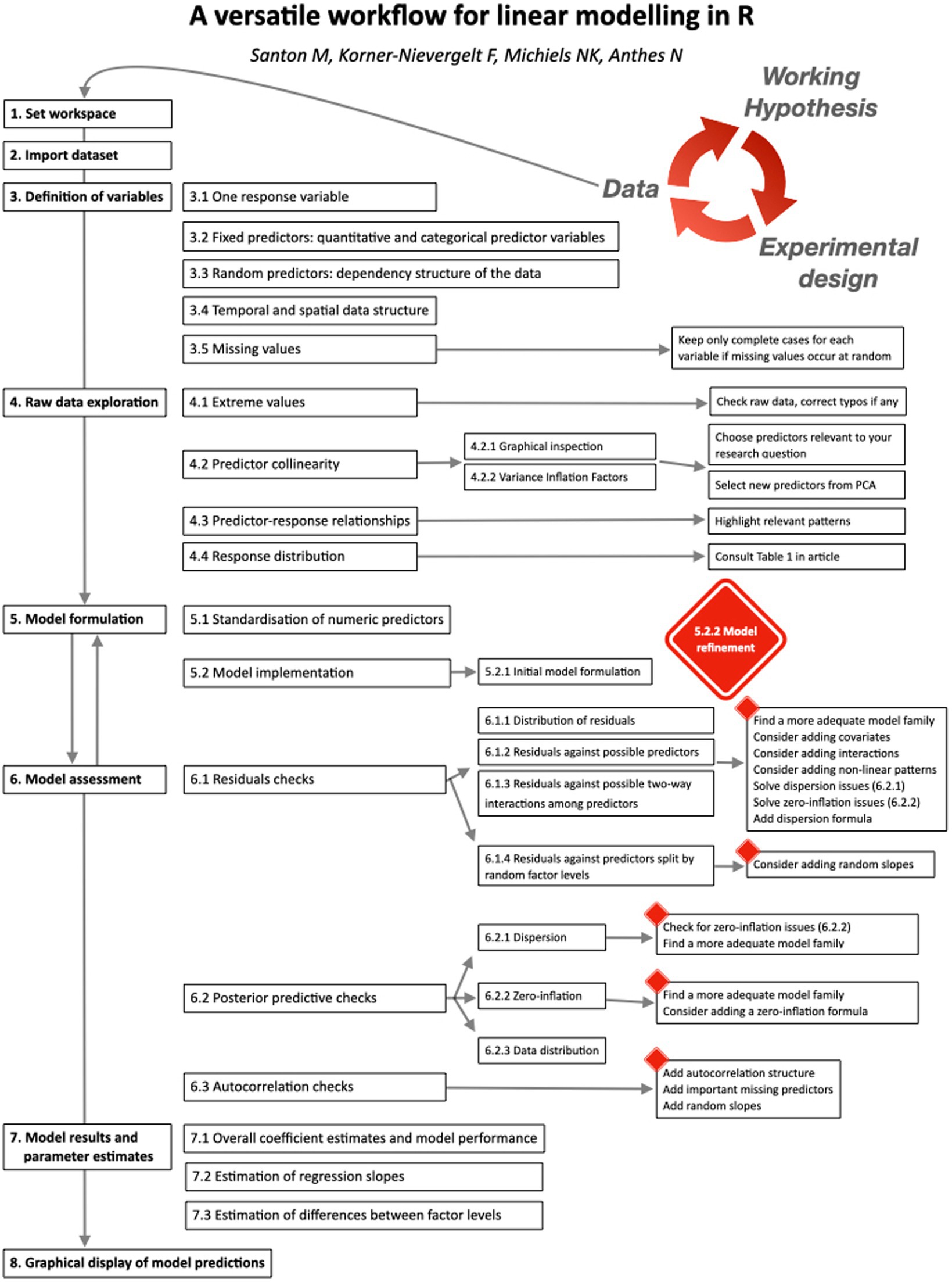
Figure 1. Flowchart for the presented linear modelling workflow.
3. Definition of variables
All variables considered for the model must be part of a single R dataframe. Users assign all dataframe columns that might be relevant for their model to any of the labels listed below. Specifying a response variable is compulsory. Labels with no variable assigned should be defined as not available (NA).
3.1. One response variable
The first object, var_resp, requires the name of a single response variable of vector class numeric or integer. This can be any quantitative measure, but also a binary response such as presence/absence, dead/alive, or failure/success coded as zeros and ones (examples in Table 1).
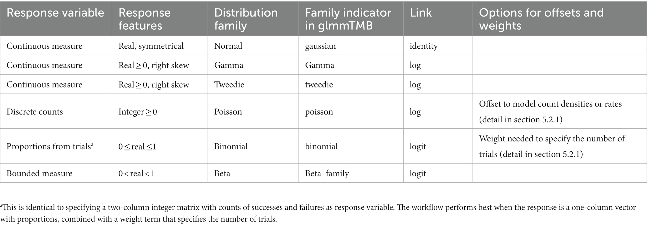
Table 1. Recommended response distribution families and link functions for initial model formulation. See Table 2 in section 6 for possible refinements after model assessment.
3.2. Fixed predictor variables
Fixed predictors may include any quantitative (i.e., numerical covariates) or categorical variables (i.e., factors) that are used to predict variation in the response variable (cf. Bolker et al., 2009). They can describe properties of study subjects (e.g., body size) or the experimental design (e.g., treatment groups).
• var_num: Name(s) of quantitative predictor variable(s), assigned to vector classes numeric or integer.
• var_fac: Name(s) of categorical predictor variable(s) with defined grouping levels, assigned to vector class factor.
3.3. Random predictor variables
Linear models assume that observations are independent (Hurlbert, 1984), i.e., that the response measure of a given replicate is independent of any other such measurement for the given (combination of) predictor(s). This assumption is usually violated when study subjects are measured repeatedly or datasets contain a spatial or temporal structure, e.g., among replicated experimental blocks or sequential sampling bouts. Ignoring such dependencies among observations in a statistical analysis generates pseudoreplication (Hurlbert, 1984; Zuur and Ieno, 2016; Colegrave and Ruxton, 2018; Harrison et al., 2018), and thus an underestimation of the uncertainty associated with the estimated model parameters (Korner-Nievergelt et al., 2015). Linear models can account for such dependencies when the dependency structure of the data is known, and adequately specified in the statistical model (Zuur et al., 2010; Harrison et al., 2018).
• var_rand: Name(s) of categorical variable(s), assigned to vector class factor, which characterise dependencies among observations.
Detailed guidance on fixed and random predictors is available elsewhere (Gelman and Hill, 2007; Harrison, 2015; Harrison et al., 2018, see also section 5.2.1). Here, we emphasize three caveats: (1) Random predictors should contain at least five levels to allow reliable estimation of between-level variance (Gelman and Hill, 2007; Harrison, 2015; Harrison et al., 2018). Otherwise, they should be added as fixed predictors in var_fac, bearing in mind that this leads to model results that cannot be generalised beyond those specific few levels. Note that even with more than five (but still rather few) levels, random factors may generate overly narrow standard errors for coefficient estimates of fixed predictors (detail in Silk et al., 2020). (2) Adding random predictors does not automatically remove every source of pseudoreplication – it is essential that the (combination of) random predictors correctly reflects the dependency structure in the data. (3) When the model contains at least two random predictors, we recommend defining each level with a unique label to avoid misspecification of nested random predictors. For example, five replicate study sites for each experimental block (from A to G) should be labeled from 1 to 5 in block A, from 6 to 10 in block B, etc., and not as repetitive labels 1 to 5 in each block.
3.4. Temporal and spatial data structure
In this step, users optionally can specify variables that describe temporal or spatial structure in their data. These variables will be used to assess temporal or spatial autocorrelation in model residuals (see section 6.3), a potential source of non-independence that usually generates overly narrow precision estimates. Note that autocorrelation can arise even if the spatial or temporal variables are also specified as fixed predictors in the model.
• var_time: Name of one numeric vector that specifies temporal information (e.g., sampling year, date, or time).
• var_time_groups (optional): Name of one factor vector that structures var_time for multiple independent time series.
• var_space: Names of two numeric vectors that specify spatial information on sampling locations as x- and y-coordinates. Both coordinates should be expressed in the same units, and preferably derive from a (roughly) equidistant projection (such as UTM or Gauss-Krueger).
3.5. Missing values
Missing values are dataframe entries with no available value (i.e., NA). Because NAs are problematic for model computation, the script excludes by default rows with a missing value for any of the variables specified in the previous steps. Missing values should not occur disproportionally often in particular data subgroups (e.g., a higher fraction of NAs for a particular sex, life-stage, species or study site). The script generates a separate dataframe that contains all excluded data rows, which allows users to check this assumption.
4. Raw data exploration
The script guides users to screen raw data for any pattern that may affect model formulation. We focus on graphical over numerical exploration in accordance with common practice in the field (Gelman et al., 2002; Quinn and Keough, 2002; Läärä, 2009; Zuur et al., 2010; Ieno and Zuur, 2015; Montgomery et al., 2021).
4.1. Extreme values
Extremes are values that are clearly smaller or larger than most other observations. Such values deserve specific attention because they may strongly influence model parameter estimates (Zuur et al., 2013a).
4.1.1. Extremes in numerical variables
We use dotplots (Cleveland, 1993) to reveal extremes in quantitative variables, i.e., the response variable and all numeric or integer predictor variables. Dotplots display the row number of each observation (yi) against its value (xi). Points that clearly isolate left or right of the core distribution deserve attention. Implausible extremes that can be objectively explained by an erroneous measurement or a typing error should be corrected or deleted. All other extremes must be kept (Zuur et al., 2010). To model such remaining extremes in the response variable without transforming the data, we recommend consulting Table 1 to select an (initial) distribution family (Zuur et al., 2010). For predictor variables, the unwanted influence of extremes on model estimation can be mitigated with data transformation, e.g., log(x + 1). Note, however, that data transformation inevitably changes the meaning – and thus interpretation – of model coefficients (Zuur et al., 2010).
4.1.2. Extremes in factor variables
For all factor predictors and random effects, we produce bar charts to reveal striking imbalances in sample sizes among factor levels. Users can reduce such imbalances by pooling factor levels with few replicates, where meaningful, or accept that effect estimates for factors with small sample sizes will associate with increased uncertainty, i.e., wide standard errors.
4.2. Predictor collinearity
Predictor values are often correlated, particularly in observational studies. This complicates the interpretation of the (partial) effects of these predictors and can substantially increase the uncertainty associated with effect estimates (Korner-Nievergelt et al., 2015). We provide graphical (4.2.1) and numerical (4.2.2) support to assess the degree of predictor collinearity.
4.2.1. Graphical inspection
The script generates default plots that allow graphical inspection of predictor collinearity with scatterplots, swarm-plots and mosaic plots for all pairwise combinations of the numeric and factor predictor variables defined in section 3. Predictor independence can be identified when datapoints spread homogeneously across the value ranges (or factor levels) of both predictors. Clear deviations indicate collinearity.
4.2.2. Variance inflation factors
Variance Inflation Factors (VIF, implementation based on Zuur et al. (2010)) quantify the inflating effect of collinearity on the standard errors of parameter estimates. Entirely independent predictors yield VIF = 1, while larger VIF values indicate increasing predictor collinearity. The treatment of collinear predictors should not solely depend on arbitrary VIF thresholds, but also on the intended interpretation of model parameters.
First, correlated predictors might represent proxies of a ‘core predictor’ that we cannot measure directly. For example, we may be interested in effects of ‘body size’, and measure weight and length to capture two of its main components. Here, users may prefer to select one of their original predictors, or to combine both using a Principal Component Analysis PCA (James and McCulloch, 1990). The first Principal Component (PC1) can then serve as a single model predictor that captures variation in ‘body size’ (Harrison et al., 2018).
Second, users may be explicitly interested in partial effects, e.g., the added effect of weight on the response variable after taking the effect of length into account. In that case, correlated predictors should be kept in the model. Note that the inclusion of correlated predictors affects model interpretation and may generate situations where models predict for (combinations of) predictor values that are beyond those present in the studied population (Morrissey and Ruxton, 2018; Gelman et al., 2020).
4.3. Predictor-response relationships
In this step, the script produces graphs of pairwise raw data relationships between the response and each potential predictor defined in section 3. These plots may reveal patterns in the raw data such as non-linear relationships and are helpful for initial model formulation and refinement in sections 5.2.1 and 5.2.2.
4.4. Response distribution
Users can “force” their response variables to approach normality with transformations (O’Hara and Kotze, 2010). However, transformations can change the relationship between response and predictor variables (Zuur et al., 2009; Duncan and Kefford, 2021) and may fail to improve model fit (O’Hara and Kotze, 2010; Warton and Hui, 2011). We therefore encourage users to rather choose the most appropriate residual distribution family for their model (Bolker, 2008; O’Hara and Kotze, 2010; Fox, 2015; Warton et al., 2016; Dunn and Smyth, 2018; Harrison et al., 2018). Users can identify a suitable initial distribution family based on (1) general considerations on the expected distribution for their type of response measure (guidance in Table 1) and (2) the distribution of the sample, provided it is sufficiently large and representative. The script displays such distribution as a raw data histogram to visually reveal skew or excess of zeroes.
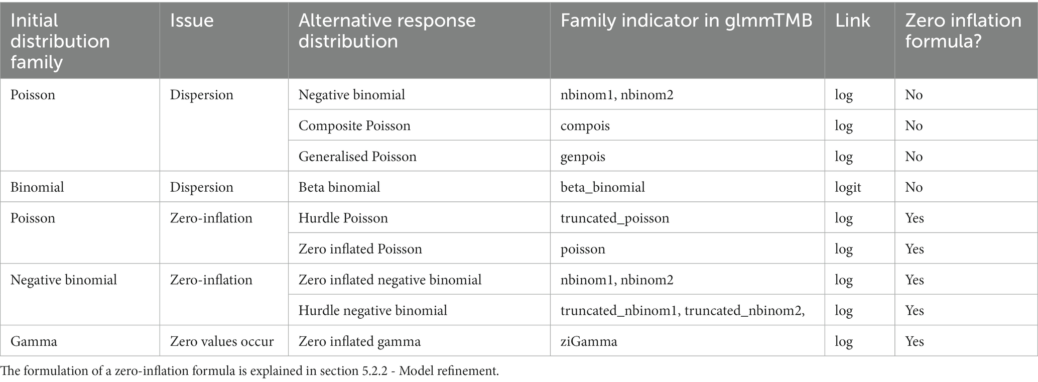
Table 2. Alternative distribution families to account for issues with dispersion or zero-inflation.
For example, users may initially select a Gaussian distribution for continuous measures with a roughly symmetrical distribution (e.g., acceleration, weight, or temperature). A Poisson distribution is a reasonable start for counts, and a binomial distribution for presence-absence data or proportions derived from counts (Harrison et al., 2018; Douma and Weedon, 2019; Table 1). Users assess (section 6) and—if needed—refine this initial choice with a new distribution in an iteration of section 5.
For each distribution family, users must specify a link function (e.g., log, logit, or identity links; Buckley, 2015). Link functions assure that model predictions for asymptotic predictor-response relationships on the raw data scale (e.g., bounded by zero for counts, and by zero and one for proportions) become linear on the link scale where the linear model coefficients are estimated (Harrison et al., 2018; Corlatti, 2021). Each response distribution has a default link function (Table 1), but other links are possible (Bolker, 2008).
5. Model formulation
In this workflow, we recommend informing initial model formulation from the biological question of interest. First, all predictors involved in a researcher’s hypothesis or study goal must be integrated as fixed predictors, including relevant interaction or polynomial terms. Second, where prior knowledge indicates that relevant variation in the response variable may associate with covariates (e.g., body size), interactions (e.g., the association of a main study predictor with the response likely varies with sex, age, or habitat) or polynomials (e.g., the association with size may possibly be quadratic instead of linear), these additional predictors should be included in the model. Third, any variable that describes dependency structures of the data must be integrated as random predictor in the model.
An alternative approach selects from a broad range of models or combines models for multi-model inference (Hooten and Hobbs, 2015). However, there is evidence that such ‘test-qualified pooling’ can generate overly confident effect estimates (Burnham and Anderson, 2007; Colegrave and Ruxton, 2017), and we therefore refrained from integrating model selection and multi-model inference in our workflow. Yet, indicators for model performance based on information theory (e.g., AIC) and multi-model inference can be instrumental when models primarily serve for prediction rather than inference (e.g., Tredennick et al., 2021).
5.1. Standardization of numeric predictors
We recommend standardizing numeric predictors before initial model formulation. Standardization often mitigates problems with model convergence, facilitates comparisons of coefficient estimates between predictors measured in different units, and assures that covariate intercepts are estimated at their population mean value (Gelman and Hill, 2007; Schielzeth, 2010; Korner-Nievergelt et al., 2015; Harrison et al., 2018). The script offers the option to z-transform all quantitative predictor variables (var_num, 3.2), where predictor means are subtracted from observed values and divided by the predictor’s standard deviation. Such z-transformed numeric predictors are expressed in units of standard deviations. Users must yet be aware that model coefficients will then be expressed as regression slopes per unit change in predictor standard deviation (rather than per original measurement unit), and that predictions for new covariate values need to be standardised with the original population mean and SD.
5.2. Model implementation
5.2.1. Initial linear model formulation
Users can now formulate their initial model. We briefly explain how to code some essential terms in glmmTMB but recommend consultation of Brooks et al. (2017) for in-depth guidance.
Our basic linear model example has two additive fixed predictors, pred.1, and pred.2:
Interaction terms for fixed predictors are specified with colons, here exemplified for a two-way interaction. We recommend restricting initial models to interaction terms that are relevant for the biological question investigated or required by study design (see above). Model assessment (Section 6) will reveal whether adding more interaction terms should be considered:
Note that when interactions are added, all lower-level interaction terms (present when interactions of higher level than two-way interactions are specified) and main predictors must be part of the model.
Random predictors can be included as random intercepts only, or as random intercepts with random slopes (Gelman and Hill, 2007; Harrison, 2015; Harrison et al., 2018). Random intercepts estimate differences between the overall response mean and the mean values of each random level (e.g., study site ID, individual ID). A random intercept effect (e.g., rand.1) is added to the model as follows:
Random intercepts assume that the fixed predictors’ effects (i.e., regression slopes or differences in group means) are consistent among random predictor levels. However, if such effects vary between random levels, models must specify random slope terms to integrate the variation in model coefficients among random levels (Korner-Nievergelt et al., 2015; Harrison et al., 2018; Silk et al., 2020). Ignoring random slopes otherwise produces overly confident effect size estimates (Schielzeth and Forstmeier, 2009; Barr et al., 2013; Aarts et al., 2015). We thus recommend initial models to specify random slopes in such situations. Note that models may fail to converge when the sample size per random level is very low (below 3) or unbalanced, which reflects the need for experimental designs with a higher number of replications per random level (Silk et al., 2020). Random slopes for a fixed predictor (e.g., pred.1) for each level of a random predictor (e.g., rand.1) are coded as follows:
Response distribution and link function are specified using the family argument, as exemplified for a Gamma response distribution with a log-link scale:
Offsets are predictors whose coefficients (= slopes) are set to 1. Hence, they are constrained to a 1 to 1 relationship with the response variable. Offsets are used to model densities or rates when the response variable represents counts. The offset variable transforms counts into densities (e.g., when the offset specifies areas or volumes) or rates (e.g., when the offset specifies transect lengths, exposure durations, or numbers of replicate surveys; Korner-Nievergelt et al., 2015). Offset terms do not need to be z-transformed as the numeric predictors, but need to be transformed with a function that is identical to the model link function. This is the logarithm in the above example scenarios, where models would use a Poisson or negative-binomial distribution family. The offset term should be specified as a separate term in the model formula as exemplified for a negative binomial model:
Weights modulate how much each observation contributes to the model. Weighting is appropriate when response values (1) are derived measures such as proportions coming from different sample sizes, or (2) vary in measurement precision. A common example for (1) is proportions of successes per individual from a variable number of replicated trials. In glmmTMB, the number of trials can be added as a weight to the binomial model (Table 1). An example for (2) is species mean sizes that have been calculated from a variable number of individuals per species and thus vary in measurement precision. This is typically accounted for by adding the inverse of the observed, squared standard error per observation as a weight (Brooks et al., 2017). As with offsets, for our routine weights should be added as separate term in the model formula as follows:
If users encounter warnings or errors while running the model, they can look for detailed guidance from the throubleshooting article that comes with glmmTMB1.
5.2.2. Model refinement
After assessing model fit (see section 6), the initial model formulation may need refinement. This may require additional model components as described in the following section.
Zero inflation describes an excess of zero values in the response variable beyond those expected by the distribution family [Zuur et al. (2013b) for more information]. When posterior predictive checks in model assessment (6.2.2) reveal zero inflation, users should consider adding a ziformula argument to the model. If the excess of zeroes distributes homogenously across predictor values, it suffices to implement ziformula = ~ 1. Otherwise, the ziformula argument can contain (combinations of) fixed or random effects to model heterogeneity in the zero distribution across predictors. The following example models an access of zeroes that varies across values of pred.1:
Dispersion formulas can be added when model assessment indicates heterogeneous residual dispersion across predictor values (6.1) that cannot be resolved by selecting a different model distribution family. Dispformula can be added to the model in a similar way as described for the ziformula above, except that it can only contain fixed effects. The example allows dispersion to vary across the values of pred.1:
Correlation (or covariance) structures offer solutions when assessment step 6.3 reveals temporal or spatial autocorrelation in model residuals. Temporal autocorrelation is often captured well by an Ornstein-Uhlenbeck (ou) covariance structure, which accommodates time series with irregularly or regularly spaced time points. The glmmTMB formulation ou(time + 0|group) requires two novel elements: “time” is a matrix of Euclidean distances that users can calculate from var_time using the function numFactor. “group” is either the vector already specified in var_time_groups, or, in case of single time series, a new factor vector with a single grouping level.
Treatment of spatial autocorrelation is a very complex topic (Banerjee et al., 2014) that faces limitations concerning computational abilities (Simpson et al., 2012) and the stability of fixed effect estimates (Hodges and Reich, 2010) that are beyond the scope of this overview. Note that, in some cases, the addition of covariates (e.g., habitat types) can already efficiently deal with spatial autocorrelation. Beyond that, users should consult the article on covariance structures that comes with the glmmTMB vignette (Brooks et al., 2017) and more advanced literature on spatial autocorrelation (e.g., Dupont et al., 2022).
6. Model assessment
Before inspecting model coefficients and effect sizes, users should assess how well the model captures patterns in the raw data and fulfils model assumptions (Freckleton, 2009; Gelman et al., 2013, 2020; Zuur and Ieno, 2016). The script guides users through graphical inspection with residual checks (6.1), posterior predictive checks (6.2), and variograms to assess residual independence across temporal or spatial scales (6.3).
Model assessment may often call for a refined model that contains other interaction or polynomial terms, or additional predictors (back to section 5). These newly added terms can increase the reliability of model estimates for the predictors specified in the initial model, but their (unexpected) effects should not be used to test new hypotheses. This would cause selection bias and increase the risk of drawing false conclusions (Forstmeier et al., 2017). Users should therefore explicitly name all terms that have been added to the model after model assessment.
6.1. Residual checks
Linear models assume that residuals are independent of predicted mean values and distribute homogeneously across all (combinations of) predictor variables. Conformity to these assumptions is visible as an absence of patterns in residual plots, and is a fundamental step of linear modelling to avoid systematic bias in parameter and uncertainty estimates (Gelman and Hill, 2007; Zuur et al., 2009; Zuur and Ieno, 2016; Gelman et al., 2020). The script displays randomised quantile residuals (Dunn and Smyth, 1996; Gelman and Hill, 2007; Dunn and Smyth, 2018) computed using the R package DHARMa (Hartig and Lohse, 2020). These residuals distribute uniformly between 0 and 1, and thus allow to evaluate residuals plots irrespective of the chosen distribution family (Hartig and Lohse, 2020).
6.1.1. Distribution of residuals
The script first produces two residual plots. The first is a quantile-quantile (Q-Q) plot (Figures 2A,B), where residuals match the expected distribution when they follow the diagonal line closely (Figure 2B). The second displays residuals against model-predicted values (Figures 2C,D), where points should scatter homogeneously without pattern (Figure 2D) (Korner-Nievergelt et al., 2015; Corlatti, 2021). Heterogeneity in residuals typically shows as a curvature or s-shape in Q-Q plots (Figure 2A), or as a change in residual spread along model predictions on the x-axis in residuals vs. fitted values plots (Figure 2C). Such models can produce biased parameter estimates and usually have overly narrow standard errors (Quinn and Keough, 2002; Fox, 2015; Zuur and Ieno, 2016). Issues are often resolved by using a more appropriate distribution family or link function (Tables 1, 2), but other possible solutions are listed in the R script (Korner-Nievergelt et al., 2015; Harrison et al., 2018).
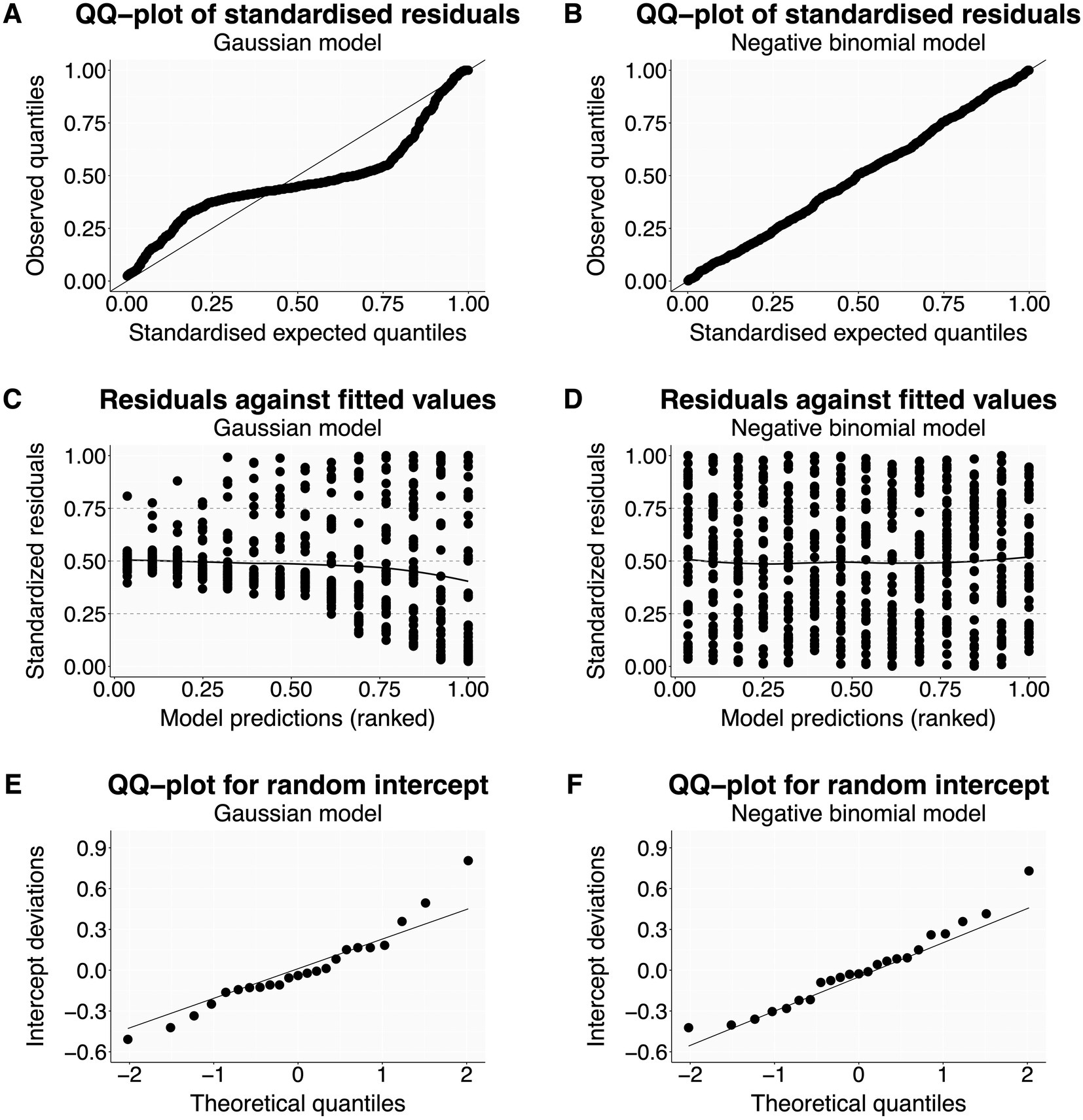
Figure 2. Distribution of residuals—examples. The left column shows residual plots for a Gaussian model with clear violations of model assumptions (A,C,E). The right column shows the same residuals plots—now without issues after changing the distribution family to negative binomial (B,D,F). The dataset from Price et al. (2016) is available with the R package glmmTMB (Brooks et al., 2017).
If the model contains random predictors, this function also generates a Q-Q plot for each predictor to check if the estimated intercepts are normally distributed (Figures 2E,F; Korner-Nievergelt et al., 2015; Harrison et al., 2018). Note that linear models are rather robust against moderate violations of normality for random intercepts (Schielzeth et al., 2020), at least as long as they are used to estimate between-group variation and are not used to make predictions for unobserved random levels.
6.1.2. Residuals against possible predictors
In this section, the script produces plots of model residuals against all fixed predictors specified in Section 3. We recommend checking residuals against all variables in the dataset, including those that are not part of the current model. Any predictor that shows residual patterns (as detailed in 6.1.1) requires further attention.
Predictors already in the model may require the addition of a curvilinear (polynomial) term, which should be added up to the desired degree using the poly function in R (Korner-Nievergelt et al., 2015). Note that high-order polynomial terms can perform poorly in regions of a dataset where data is sparse (Wood, 2017) and should thus be used with care (Gelman et al., 2020). If the dataset features more complex non-linear patterns, we recommend resorting to dedicated R packages such as mgcv (Wood, 2017) to implement more appropriate models.
Predictors not yet included in the model that show residual patterns should be added to help explaining variation in the response variable (see above).
6.1.3. Residuals against possible two-way interactions among predictors
The script produces residual plots for all two-way combinations of fixed predictors. Heterogeneous residual patterns beyond those already seen above identify predictor combinations that may need addition as an interaction term to the refined model formulation, provided the original question being asked is not altered.
6.1.4. Residuals against predictors split by random factor levels
Finally, the script helps users to evaluate if a random intercept needs the addition of random slopes over a specific fixed predictor (Korner-Nievergelt et al., 2015). This residual check is relevant only for fixed predictors with 3 or more observations per random level. The plots generated by the script show the distribution of model residuals across the selected predictors, split by the levels of the specified random intercept predictor(s). If panels show diverging slopes for numeric predictors or inconsistent effect directions for categorical predictors, the model requires the addition of random slopes for that predictor (Schielzeth and Forstmeier, 2009; Silk et al., 2020) to avoid overly confident coefficient estimates (Schielzeth and Forstmeier, 2009). Note that residual mean values per random level do not need to be zero: Due to the shrinkage estimation of mean values per random effect level, average residuals can be positive for levels with low means, and negative for levels with high means.
6.2. Posterior predictive checks
Even careful residual assessment may leave several important aspects of model fit unexplored (Faraway, 2016; Pekár and Brabec, 2016). Therefore, we assess model performance also with posterior predictive checks, which compare the observed data with the distribution of many (e.g., 2000) replicated datasets simulated from the model (Gelman and Hill, 2007; Gelman et al., 2013; Zuur and Ieno, 2016). The script guides users to graphically evaluate dispersion (6.2.1), zero-inflation (6.2.2) and overall model fit (6.2.3; Figure 3). These plots display observed parameters as blue lines when they are within the central 90% of the simulated distribution (labeled as ‘optimal fit’), orange lines when between the central 90% and 99% boundaries (‘sub-optimal fit’), and red lines when outside the central 99% boundaries (‘poor fit’). These boundaries are set arbitrarily to provide qualitative guidance. We recommend seeking an optimal fit while bearing in mind that model performance is seldom perfect for all parameters at once.
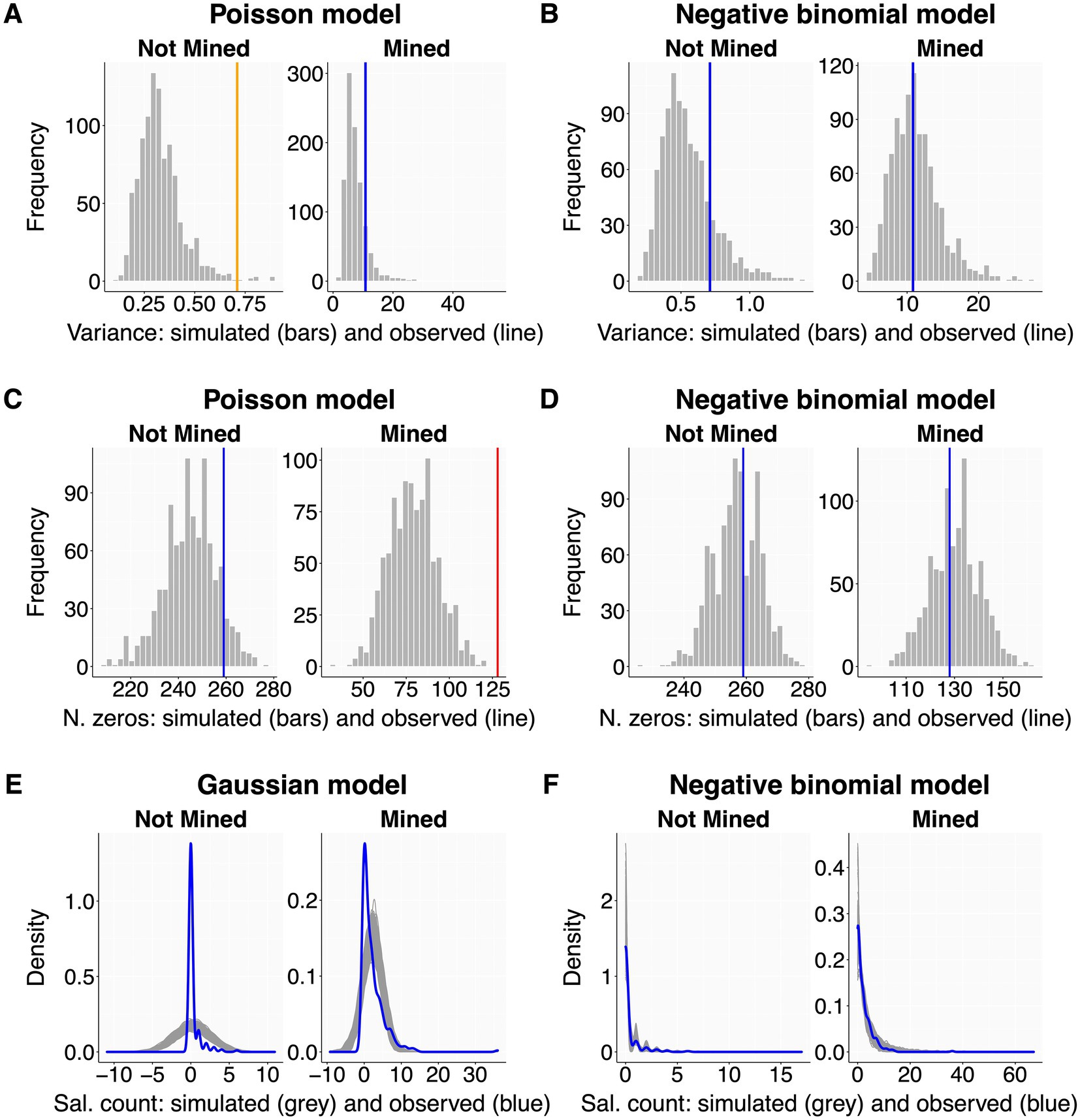
Figure 3. Posterior predictive checks - examples. All plots show observed values or data distributions (thick colored lines) in relation to those obtained from 10,000 simulations of raw datasets from the model. Each panel is split by a categorical predictor with two levels (sites without and with mining activity). The left column shows clear deviations between observed and simulated data for dispersion (A), number of zeros (C), and overall data distribution (E). The right column has all issues solved by changing distribution family from Poisson to negative binomial for (B) and (D), and from Gaussian to negative binomial for (F). A Gaussian distribution was here chosen only to create a clear deviation for display purposes. Dataset as in Figure 2.
6.2.1. Dispersion
Some response distributions (e.g., Poisson and binomial) assume tight coupling between mean and variance, an assumption that is often violated (Cox, 1983; Yang et al., 2010). Over- or underdispersion arises when the data (and residual) variation is higher or lower than predicted from the population mean. Both can lead to biased parameter estimates and inappropriately small (or large) standard errors (Hilbe, 2011; Zuur and Ieno, 2016; Campbell, 2021). The script graphically compares the variance of the observed data with the variance distribution of model-simulated datasets (Figures 3A,B). We recommend users to split this plot by the levels of each categorical predictor used in the model, because dispersion should also be checked within each factor level.
Dispersion issues can originate from an inappropriate distribution family, a wider spread of the data than expected by the observed mean, or an excess of zero values (Harrison, 2014). Dispersion checks should therefore always go along with zero-inflation checks (6.2.2). Potential solutions include a distribution family that better captures the observed data dispersion (Table 2; Hilbe, 2011; Harrison, 2015; Harrison et al., 2018) or that adequately integrates the excess of zeroes (Yang et al., 2010).
6.2.2. Zero-inflation
Here, the script visualises the observed number of zero values against the zero-distribution derived from model-simulated datasets (Figures 2C,D). Users should split displays by factor levels as described for dispersion (6.2.1). If deviations are detected, users may choose a distribution family that better captures the observed zero frequencies (Table 2) or add a zero-inflation formula to the model (5.2.2).
6.2.3. Data distribution
This final posterior predictive check evaluates overall model fit (Gelman et al., 2013; Zuur and Ieno, 2016). The script plots the density of the observed data distribution (blue line) against that of model-simulated datasets (gray lines; Figures 3E,F), ideally split by the levels of each factor predictor as before. The observed (blue) line should be central within the gray background pattern of simulated data. If this is clearly not the case, users should carefully re-evaluate all preceding steps of model assessment and reformulate their model accordingly (back to section 5).
6.3. Autocorrelation checks
Ecological sampling often has a temporal or spatial component. This may introduce dependency structures in the response variable where observations closer in time or space are more similar (Zuur et al., 2010; Korner-Nievergelt et al., 2015), leading to pseudoreplication. To assess whether such temporal or spatial autocorrelation is present in the data, the script produces graphical autocorrelation checks for temporal (based on var_time and var_time_groups from 3.4) or spatial data structures (based on var_space from 3.4) using semivariograms (Schabenberger and Pierce, 2002). Semivariograms display how the ‘standardised semivariance’ (i.e., standardised, half squared differences in model residuals between all observation pairs) changes with the spatial or temporal distance between sample pairs (Hengl, 2007; Korner-Nievergelt et al., 2015). Standardised semivariances of fully independent observations fluctuate around 1. Smaller semivariance values identify observations that are more similar than expected at random, and thus autocorrelated. Observed semivariances are calculated using the variog function of the geoR package (Ribeiro and Diggle, 2001). To aid interpretation, we plot these (blue line) against the distribution of semivariances expected in the absence of autocorrelation, as derived from many (e.g., 2000) permutated model residuals (Figure 4). Observed standardised semivariances that clearly fall below the gray permuted pattern indicate autocorrelation. In such cases, users should consider adding a covariance structure to the model (5.2.2).
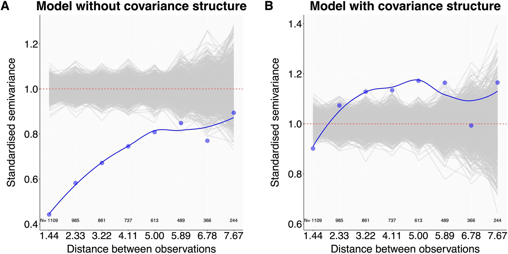
Figure 4. Autocorrelation checks - examples. Plot (A) shows that observations with a pairwise distance up to 6 have more similar residuals (blue dots and blue line) than expected at random (gray lines), indicating spatial autocorrelation. Plot (B), now almost free of autocorrelation, was produced by informing the model with the autocorrelation structure of the observations. N values are the number of observation pairs in the dataset within each distance step indicated on the x-axis. Dataset reworked from Santon et al. (2021).
7. Model results and parameter estimates
Once the iteration of model assessment and refinement resulted in an adequate model, users can finally inspect model estimates. This workflow refrains from null hypothesis tests because they offer limited information about the magnitude and biological meaning of the observed effects and bear a substantial risk of misinterpretation (Johnson, 1999; Nakagawa and Cuthill, 2007; Cumming, 2008; Halsey et al., 2015; Cumming and Calin-Jageman, 2017; Halsey, 2019). We instead focus on reporting effect sizes with their ‘compatibility intervals’ (Gelman and Greenland, 2019; Halsey, 2019; Berner and Amrhein, 2022), i.e., the central 95% density interval of effect values that are most compatible with the observed data. Berner and Amrhein (2022) offer further guidance on reporting without falling back to ‘null hypothesis testing’ terminology.
7.1. Overall coefficient estimates
The script displays coefficient estimates for each model parameter, including their 95% compatibility intervals using a custom function based on the parameters package (Lüdecke et al., 2020b). Note that parameter estimates are on the model link scale. As an alternative way of measuring effect sizes, the r2 function from the performance package (Lüdecke et al., 2020a) estimates the variance explained by the model for fixed predictors only (marginal R2), and for fixed plus random predictors (conditional R2; Nakagawa and Schielzeth, 2013; Nakagawa et al., 2017; Harrison et al., 2018).
Users may want to also report estimates of regression slopes within factor levels, or differences in predicted mean values between factor levels. We introduce functions that extract such estimates and their 95% compatibility intervals in the following two sections. We refer users to the extensive guidance provided with the emmeans package (Lenth, 2023) to compute estimates beyond the capabilities of the functions presented in the script.
7.2. Estimation of regression slopes
This section computes predicted slopes and their 95% CIs for models containing interaction terms between one numeric predictor and up to two factor predictors using a custom function based on the emmeans package (Lenth, 2023). Slope estimates per unit increase of the numeric predictor are always given on the model link scale where regression slopes are linear. For log and logit link models, we additionally provide estimates for the resulting response ratios and odds ratios, respectively. For standardised numeric predictors, slope estimates show changes per unit standard deviation of the predictor. The predicted slopes and their 95% CIs can be reported as exemplified in Table 3. Effect size strength increases with the deviation of estimates from zero (for Gaussian models, and for changes on the link scale for other model families) or one (for changes expressed as response ratios and odds ratios for log- and logit-link functions, respectively), and the robustness of the result increases the less the 95% Compatibility Intervals (CIs) overlap with zero or one, respectively. The script additionally produces a graphical output of the effect estimates with their compatibility intervals on the model link scale (examples in the Supplementary file).
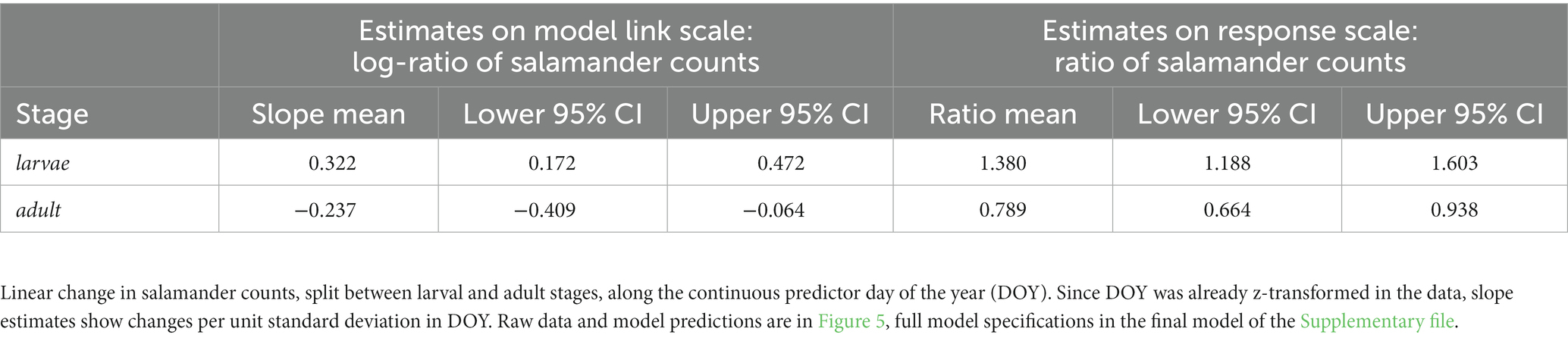
Table 3. Example of a numerical presentation of regression slopes.
7.3. Estimation of differences between factor levels
The script estimates differences in mean values either between all possible combinations of the levels of a user specified selection of factor predictors, or for the levels of one factor predictor within the levels of a second one, using a custom function based on the emmeans package (Lenth, 2023). The function displays absolute differences in mean values for identity link models, and ratios or odds ratios for log or logit link models, respectively. As above, effect estimates, and their 95% compatibility intervals are reported as a table (exemplified in Table 4) and as a graphical output (examples in the Supplementary file). Effect size and CIs interpretation is the same as described for regression slopes above.
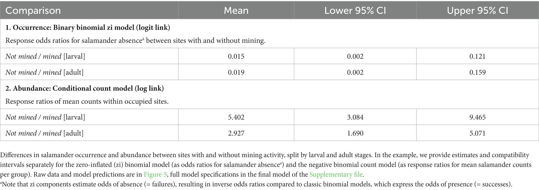
Table 4. Example for the numerical presentation of differences between factor levels.
8. Graphical display of model predictions
An intuitive and comprehensive way to visualise the relationship between response and predictor variables is a combined display of raw data with model-derived predictions and their 95% compatibility intervals (Best and Wolf, 2013; Halsey, 2019; Ho et al., 2019). The script produces such displays after users specified one or two fixed predictors (Figures 5A,B). First, the script calculates the posterior distribution of fitted values from 10,000 sets of model parameters drawn from a Multivariate Normal Distribution based on the predicted mean and variance of each model coefficient (Brooks et al., 2017). From these, the script extracts model-predicted means and their 95% compatibility intervals per factor level, or along the numeric range of the specified predictor(s) of interest, with all other predictor(s) set to their median values. Finally, the script summarises the raw data at the specified replicate level, and plot them together with predicted means and compatibility intervals (Korner-Nievergelt et al., 2015; Brooks et al., 2017).
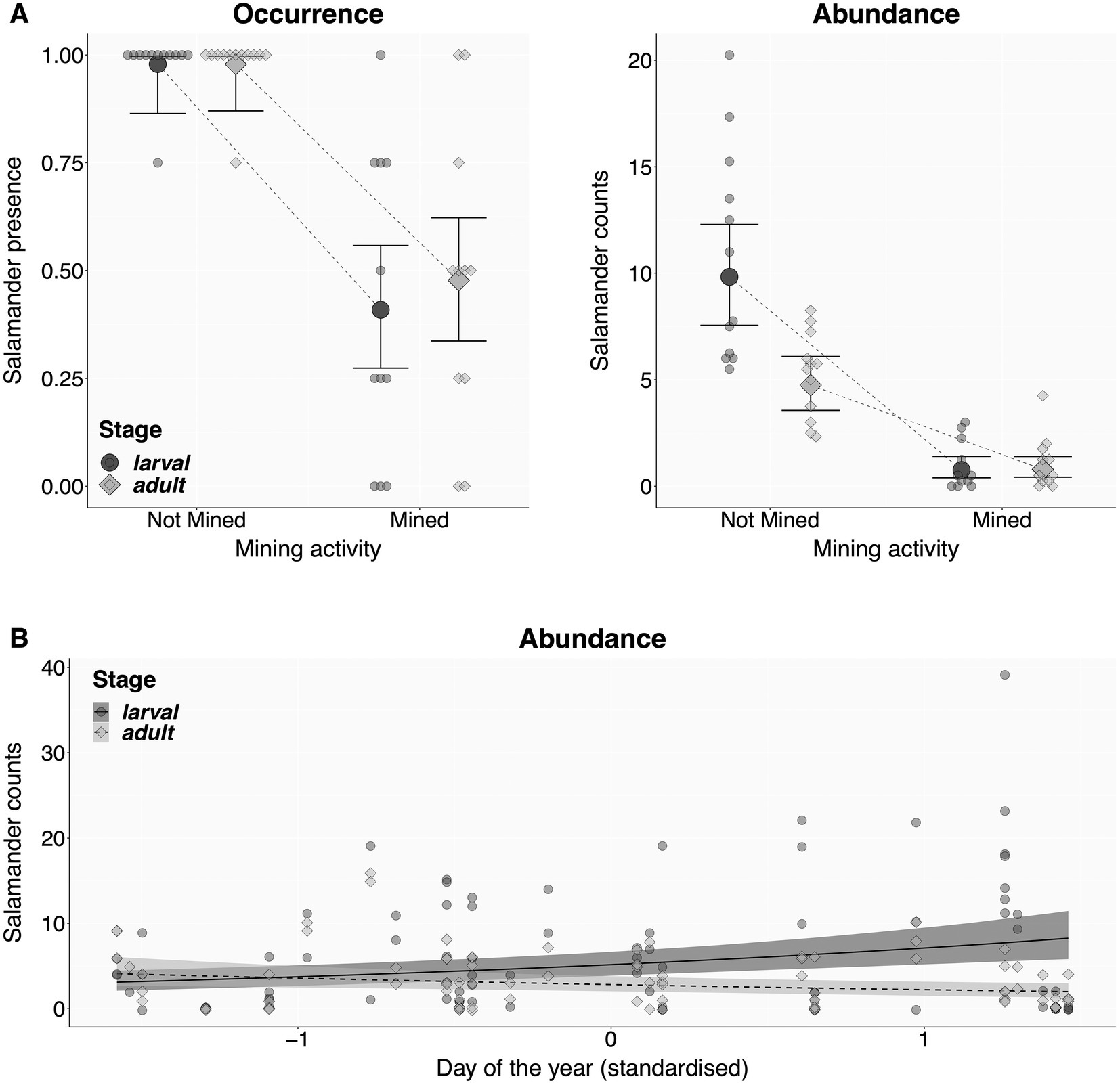
Figure 5. Salamander individual counts as a function of salamander stage and mining activity (A), and salamander stage and day of the year (B). Each point is an average value per combination of stage, site, and mining activity (N = 23 sites, representing the true replicates), showing either the proportion of four repeated surveys with at least one individual present (A: Occurrence), or the mean salamander count (A,B: Abundances). Mean model predictions (filled markers or shades) and their 95% compatibility intervals (bold lines) were derived from 10,000 simulations of the posterior distribution of model parameters.
Author’s note
The most recent version of the template and support functions R-scripts will be available for download on GitHub: https://github.com/MSSanton/glmms_workflow.
Data availability statement
The original contributions presented in the study are included in the article/supplementary material, further inquiries can be directed to the corresponding author.
Author contributions
MS and NA conceived the study, coded the R-workflow, and wrote the manuscript. MS analyzed the data. MS, NA, and FK-N tested the R-workflow. FK-N and NM edited the manuscript it. All authors contributed to the article and approved the submitted version.
Funding
This work was supported by the Engineering and Physical Sciences Research Council [grant number EP/X020819/1 awarded to MS].
Acknowledgments
The development of this workflow has greatly profited from students and researchers who shared their unpublished datasets and provided feedback on the routine: Fabian Anger, Jonathan Bauder, Felix Deiss, Leonie John, Thomas Kimmich, Stefanie Krais, Franziska Lehle, Laura-Sophia Limmer, Franziska Mück, Katharina Peschke, Federica Poli, Anaelle Regen, and Bram van der Schoot. We further thank Xavier Harrison, Jakob Katzenberger, Roger Mundry, and Eric Jason Pedersen for insightful comments that improved the quality of this work.
Conflict of interest
FK-N was employed by the company Oikostat GmbH.
The remaining authors declare that the research was conducted in the absence of any commercial or financial relationships that could be construed as a potential conflict of interest.
Publisher’s note
All claims expressed in this article are solely those of the authors and do not necessarily represent those of their affiliated organizations, or those of the publisher, the editors and the reviewers. Any product that may be evaluated in this article, or claim that may be made by its manufacturer, is not guaranteed or endorsed by the publisher.
Supplementary material
The Supplementary material for this article can be found online at: https://www.frontiersin.org/articles/10.3389/fevo.2023.1065273/full#supplementary-material
Footnotes
References
Aarts, E., Dolan, C. V., Verhage, M., and van der Sluis, S. (2015). Multilevel analysis quantifies variation in the experimental effect while optimizing power and preventing false positives. BMC Neurosci. 16, 1–15. doi: 10.1186/s12868-015-0228-5
Banerjee, S., Carlin, B. P., and Gelfand, A. E. (2014). Hierarchical Modelling and analysis for spatial data, 2nd edn. Taylor & Francis, London.
Barr, D. J., Levy, R., Scheepers, C., and Tily, H. J. (2013). Random effects structure for confirmatory hypothesis testing: keep it maximal. J. Mem. Lang. 68, 255–278. doi: 10.1016/j.jml.2012.11.001
Berner, D., and Amrhein, V. (2022). Why and how we should join the shift from significance testing to estimation. J. Evol. Biol. 35, 777–787. doi: 10.1111/jeb.14009
Best, H., and Wolf, C. (2013). The SAGE handbook of regression analysis and causal inference. SAGE Publications, Los Angeles, CA.
Bolker, B. (2015). “Linear and generalized linear mixed models,” in Ecological statistics: Contemporary theory and application. eds. G. A. Fox, S. Negrette-Yankelevich, and V. J. Sosa (Oxford, UK: Oxford University Press), 309–333.
Bolker, B. M., Brooks, M. E., Clark, C. J., Geange, S. W., Poulsen, J. R., Stevens, M. H. H., et al. (2009). Generalized linear mixed models: a practical guide for ecology and evolution. Trends Ecol. Evol. 24, 127–135. doi: 10.1016/j.tree.2008.10.008
Breheny, P., and Burchett, W. (2017). Visualization of regression models using visreg. RJ 9:56. doi: 10.32614/RJ-2017-046
Brooks, M. E., Kristensen, K., van Benthem, K. J., Magnusson, A., Berg, C. W., Nielsen, A., et al. (2017). glmmTMB balances speed and flexibility among packages for zero-inflated generalized linear mixed modelling. R J 9, 378–400. doi: 10.32614/RJ-2017-066
Buckley, Y. M. (2015). “Generalized linear models” in Ecological statistics: Contemporary theory and application. eds. G. A. Fox, S. Negrete-Yankelevich, and V. J. Sosa (Oxford, UK: Oxford University Press), 131–148.
Burnham, K. P., and Anderson, D. R. (2007). Model selection and multimodel inference: a practical information-theoretic approach, Springer New York.
Campbell, H. (2021). The consequences of checking for zero-inflation and overdispersion in the analysis of count data. Methods Ecol. Evol. 12, 665–680. doi: 10.1111/2041-210X.13559
Colegrave, N., and Ruxton, G. D. (2017). Statistical model specification and power: recommendations on the use of test-qualified pooling in analysis of experimental data. Proc. R. Soc. B Biol. Sci. 284:20161850. doi: 10.1098/rspb.2016.1850
Colegrave, N., and Ruxton, G. D. (2018). Using biological insight and pragmatism when thinking about pseudoreplication. Trends Ecol. Evol. 33, 28–35. doi: 10.1016/j.tree.2017.10.007
Corlatti, L. (2021). Regression models, fantastic beasts, and where to find them: a simple tutorial for ecologists using R. Bioinformatics Biol. Insights 15:11779322211051522. doi: 10.1177/11779322211051522
Cumming, G. (2008). Replication and p intervals: p values predict the future only vaguely, but confidence intervals do much better. Perspect. Psychol. Sci. 3, 286–300. doi: 10.1111/j.1745-6924.2008.00079.x
Cumming, G., and Calin-Jageman, R. (2017). Introduction to the new statistics: Estimation, open science, and beyond. Routledge, Abingdon, UK.
Douma, J. C., and Weedon, J. T. (2019). Analysing continuous proportions in ecology and evolution: a practical introduction to beta and Dirichlet regression. Methods Ecol. Evol. 10, 1412–1430. doi: 10.1111/2041-210X.13234
Duncan, R. P., and Kefford, B. J. (2021). Interactions in statistical models: three things to know. Methods Ecol. Evol. 12, 2287–2297. doi: 10.1111/2041-210X.13714
Dunn, P. K., and Smyth, G. K. (1996). Randomized quantile residuals. J. Comput. Graph. Stat. 5, 236–244.
Dunn, P. K., and Smyth, G. K. (2018). Generalized linear models with examples in R. New York: Springer New York.
Dupont, E., Wood, S. N., and Augustin, N. (2022). Spatial+: a novel approach to spatial confounding. Biometrics 78, 1279–1290. doi: 10.1111/biom.13656
Faraway, J. J. (2016). Extending the linear model with R: Generalized linear, mixed effects and nonparametric regression models. CRC press, Boca Raton, FL.
Forstmeier, W., Wagenmakers, E. -J., and Parker, T. H. (2017). Detecting and avoiding likely false-positive findings – a practical guide. Biol. Rev. 92, 1941–1968. doi: 10.1111/brv.12315
Fox, J. (2015). Applied regression analysis and generalized linear models. Sage Publications, Los Angeles, CA.
Freckleton, R. (2009). The seven deadly sins of comparative analysis. J. Evol. Biol. 22, 1367–1375. doi: 10.1111/j.1420-9101.2009.01757.x
Gelman, A., Carlin, J. B., Stern, H. S., Dunson, D. B., Vehtari, A., and Rubin, D. B. (2013). Bayesian data analysis. Taylor & Francis, London.
Gelman, A., and Greenland, S. (2019). Are confidence intervals better termed “uncertainty intervals”? BMJ 366:l5381. doi: 10.1136/bmj.l5381
Gelman, A., and Hill, J. (2007). Data analysis using regression and multilevel/hierarchical models. Cambridge University Press, Cambridge UK.
Gelman, A., Hill, J., and Vehtari, A. (2020). Regression and other stories. Cambridge University Press, Cambridge UK.
Gelman, A., Pasarica, C., and Dodhia, R. (2002). Let's practice what we preach: turning tables into graphs. Am. Stat. 56, 121–130. doi: 10.1198/000313002317572790
Halsey, L. G. (2019). The reign of the p-value is over: what alternative analyses could we employ to fill the power vacuum? Biol. Lett. 15:20190174. doi: 10.1098/rsbl.2019.0174
Halsey, L. G., Curran-Everett, D., Vowler, S. L., and Drummond, G. B. (2015). The fickle P value generates irreproducible results. Nat. Methods 12, 179–185. doi: 10.1038/nmeth.3288
Harrison, X. A. (2014). Using observation-level random effects to model overdispersion in count data in ecology and evolution. PeerJ 2:e616. doi: 10.7717/peerj.616
Harrison, X. A. (2015). A comparison of observation-level random effect and Beta-binomial models for modelling overdispersion in binomial data in ecology & evolution. PeerJ 3:e1114. doi: 10.7717/peerj.1114
Harrison, X. A., Donaldson, L., Correa-Cano, M. E., Evans, J., Fisher, D. N., Goodwin, C. E., et al. (2018). A brief introduction to mixed effects modelling and multi-model inference in ecology. PeerJ 6:e4794. doi: 10.7717/peerj.4794
Hartig, F., and Lohse, L. (2020). DHARMa: residual diagnostics for hierarchical (multi-level/mixed) regression models (0.3.3.0). Available at: https://cran.r-project.org/web/packages/DHARMa/index.html
Hengl, T. (2007). A practical guide to geostatistical mapping of environmental variables. EUR 22904 EN. Luxembourg (Luxembourg): Office for Official Publications of the European Communities.
Ho, J., Tumkaya, T., Aryal, S., Choi, H., and Claridge-Chang, A. (2019). Moving beyond P values: data analysis with estimation graphics. Nat. Methods 16, 565–566. doi: 10.1038/s41592-019-0470-3
Hodges, J. S., and Reich, B. J. (2010). Adding spatially-correlated errors can mess up the fixed effect you love. Am. Stat. 64, 325–334. doi: 10.1198/tast.2010.10052
Hooten, M. B., and Hobbs, N. T. (2015). A guide to Bayesian model selection for ecologists. Ecol. Monogr. 85, 3–28. doi: 10.1890/14-0661.1
Hurlbert, S. H. (1984). Pseudoreplication and the design of ecological field experiments. Ecol. Monogr. 54, 187–211. doi: 10.2307/1942661
Ieno, E. N., and Zuur, A. F. (2015). A Beginner's guide to data exploration and visualisation with R. Highland Statistics Limited, Newburgh, NY.
James, F. C., and McCulloch, C. E. (1990). Multivariate analysis in ecology and systematics: panacea or Pandora's box? Annu. Rev. Ecol. Syst. 21, 129–166. doi: 10.1146/annurev.es.21.110190.001021
Johnson, D. H. (1999). The insignificance of statistical significance testing. J. Wildl. Manag. 63, 763–772. doi: 10.2307/3802789
Korner-Nievergelt, F., Roth, T., von Felten, S., Guélat, J., Almasi, B., and Korner-Nievergelt, P. (2015). Bayesian data analysis in ecology using linear models with R, BUGS, and Stan. Academic Press, London.
Läärä, E. (2009). Statistics: reasoning on uncertainty, and the insignificance of testing null. Ann. Zool. Fenn. 46, 138–157. doi: 10.5735/086.046.0206
Lenth, R. (2023). Emmeans: Estimated marginal means, aka least-squares means. R package version 1.8.4–1. Available at: https://CRAN.R-project.org/package=emmeans.
Lüdecke, D., Ben-Shachar, M. S., Patil, I., and Makowski, D. (2020b). Extracting, computing and exploring the parameters of statistical models using R. J. Open Source Softw. 5:2445. doi: 10.21105/joss.02445
Lüdecke, D., Ben-Shachar, M., Patil, I., Waggoner, P., and Makowski, D. (2020a). Performance: an R package for assessment, comparison and testing fof statistical models. J. Open Source Soft. 6:1139. doi: 10.21105/joss.03139
Montgomery, D. C., Peck, E. A., and Vining, G. G. (2021). Introduction to linear regression analysis. John Wiley & Sons, Hoboken, NJ.
Morrissey, M. B., and Ruxton, G. D. (2018). Multiple regression is not multiple regressions: the meaning of multiple regression and the non-problem of collinearity. Philos. Theory Pract. Biol. 10 (3). doi: 10.3998/ptpbio.16039257.0010.003
Nakagawa, S., and Cuthill, I. C. (2007). Effect size, confidence interval and statistical significance: a practical guide for biologists. Biol. Rev. 82, 591–605. doi: 10.1111/j.1469-185X.2007.00027.x
Nakagawa, S., Johnson, P. C. D., and Schielzeth, H. (2017). The coefficient of determination R2 and intra-class correlation coefficient from generalized linear mixed-effects models revisited and expanded. J. R. Soc. Interface 14:20170213. doi: 10.1098/rsif.2017.0213
Nakagawa, S., and Schielzeth, H. (2013). A general and simple method for obtaining R2 from generalized linear mixed-effects models. Methods Ecol. Evol. 4, 133–142. doi: 10.1111/j.2041-210x.2012.00261.x
O’Hara, R., and Kotze, J. (2010). Do not log-transform count data. Nat. Precedings. 1, 118–122. doi: 10.1038/npre.2010.4136.1
Pekár, S., and Brabec, M. (2016). Modern analysis of biological data: Generalized linear models in R. Masarykova univerzita, Brno, Czeh Republic.
Price, S. J., Muncy, B. L., Bonner, S. J., Drayer, A. N., and Barton, C. D. (2016). Effects of mountaintop removal mining and valley filling on the occupancy and abundance of stream salamanders. J. Appl. Ecol. 53, 459–468. doi: 10.1111/1365-2664.12585
Quinn, G. P., and Keough, M. J. (2002). Experimental design and data analysis for biologists. Cambridge university press, Cambridge UK.
R Core Team (2017). R: A language and environment for statistical computing R Foundation for Statistical Computing, Vienna, Austria.
Ribeiro, P. Jr., and Diggle, P. (2001). GeoR: a package for geostatistical anaysis. R-News 1, 1609–3631.
Santon, M., Deiss, F., Bitton, P.-P., and Michiels, N. K. (2021). A context analysis of bobbing and fin-flicking in a small marine benthic fish. Ecol. Evol. 11, 1254–1263. doi: 10.1002/ece3.7116
Schabenberger, O., and Pierce, F. (2002). Linear mixed models. Contemporary statistical models for plant and soil sciences. New York, NY: Taylor and Francis, 495–496.
Schielzeth, H. (2010). Simple means to improve the interpretability of regression coefficients. Methods Ecol. Evol. 1, 103–113. doi: 10.1111/j.2041-210X.2010.00012.x
Schielzeth, H., Dingemanse, N. J., Nakagawa, S., Westneat, D. F., Allegue, H., Teplitsky, C., et al. (2020). Robustness of linear mixed-effects models to violations of distributional assumptions. Methods Ecol. Evol. 11, 1141–1152. doi: 10.1111/2041-210X.13434
Schielzeth, H., and Forstmeier, W. (2009). Conclusions beyond support: overconfident estimates in mixed models. Behav. Ecol. 20, 416–420. doi: 10.1093/beheco/arn145
Silk, M. J., Harrison, X. A., and Hodgson, D. J. (2020). Perils and pitfalls of mixed-effects regression models in biology. PeerJ 8:e9522. doi: 10.7717/peerj.9522
Simpson, D., Lindgren, F., and Rue, H. (2012). In order to make spatial statistics computationally feasible, we need to forget about the covariance function. Environmetrics 23, 65–74. doi: 10.1002/env.1137
Taper, M. L. (2004). “Model identification from many candidates” in The nature of scientific evidence: Statistical, philosophical, and empirical considerations (Chicago: University of Chicago Press), 488–524.
Tredennick, A. T., Hooker, G., Ellner, S. P., and Adler, P. B. (2021). A practical guide to selecting models for exploration, inference, and prediction in ecology. Ecology 102:e03336. doi: 10.1002/ecy.3336
Warton, D. I., and Hui, F. K. (2011). The arcsine is asinine: the analysis of proportions in ecology. Ecology 92, 3–10. doi: 10.1890/10-0340.1
Warton, D. I., Lyons, M., Stoklosa, J., and Ives, A. R. (2016). Three points to consider when choosing a LM or GLM test for count data. Methods Ecol. Evol. 7, 882–890. doi: 10.1111/2041-210X.12552
Wood, S. N. (2017). Generalized additive models: An introduction with R. CRC Press/Taylor & Francis Group, Boca Raton, FL.
Yang, Z., Hardin, J. W., and Addy, C. L. (2010). Some remarks on testing overdispersion in zero-inflated Poisson and binomial regression models. Commun. Stat. Theory Methods 39, 2743–2752. doi: 10.1080/03610920903177397
Zuur, A. F., Hilbe, J. M., and Ieno, E. N. (2013a). A Beginner's guide to GLM and GLMM with R: A frequentist and Bayesian perspective for ecologists. Highland Statistics Limited, Newburgh, NY.
Zuur, A. F., and Ieno, E. N. (2016). A protocol for conducting and presenting results of regression-type analyses. Methods Ecol. Evol. 7, 636–645. doi: 10.1111/2041-210X.12577
Zuur, A. F., Ieno, E. N., and Elphick, C. S. (2010). A protocol for data exploration to avoid common statistical problems. Methods Ecol. Evol. 1, 3–14. doi: 10.1111/j.2041-210X.2009.00001.x
Zuur, A. F., Ieno, E. N., Walker, N., Saveliev, A. A., and Smith, G. M. (2009). Mixed effects models and extensions in ecology with R. New York: Springer.
Keywords: GLMMs, glmmTMB, linear models, model assessment, residual analysis, R-workflow, posterior predictive checks
Citation: Santon M, Korner-Nievergelt F, Michiels NK and Anthes N (2023) A versatile workflow for linear modelling in R. Front. Ecol. Evol. 11:1065273. doi: 10.3389/fevo.2023.1065273
Edited by:
Claudia Fichtel, Deutsches Primatenzentrum, GermanyReviewed by:
Roger Mundry, Leibniz ScienceCampus Primate Cognition, GermanyEric Jason Pedersen, Concordia University, Canada
Jakob Katzenberger, Dachverband Deutscher Avifaunisten, Germany
Copyright © 2023 Santon, Korner-Nievergelt, Michiels and Anthes. This is an open-access article distributed under the terms of the Creative Commons Attribution License (CC BY). The use, distribution or reproduction in other forums is permitted, provided the original author(s) and the copyright owner(s) are credited and that the original publication in this journal is cited, in accordance with accepted academic practice. No use, distribution or reproduction is permitted which does not comply with these terms.
*Correspondence: Matteo Santon, matteo.santon@bristol.ac.uk