Unsynchronized Driving Mechanisms of Spring and Autumn Phenology Over Northern Hemisphere Grasslands

Introduction

Global vegetation phenology has shifted with climate change during the recent decades (Myneni et al., 1997; Menzel et al., 2006; Schwartz et al., 2006; Zeng et al., 2011; Piao et al., 2019). Warming has been ascribed as the main driving factor (Lucht et al., 2002; Zhang et al., 2004; Piao et al., 2006; Jeong et al., 2011), and advanced vegetation green-up has been observed globally, albeit with magnitudes varying with vegetation type, study region, period, and method (White et al., 2009; Cong et al., 2012, 2013; Piao et al., 2017). Across temperate regions, increasing temperature has broken dormancy earlier and vegetation growth recovery has consistently advanced, resulting in enhanced vegetation gross primary productivity (GPP) (Keeling et al., 1996; Hu et al., 2011). In addition to spring phenology, research has been devoted also to autumn phenology (Yang et al., 2015; Liu et al., 2016), which is closely linked with vegetation productivity (Jeong et al., 2011; Garonna et al., 2014). An extended growing season directly leads to increased vegetation GPP. However, vegetation chlorophyll content decreases at the end of the growing season, and vegetation photosynthesis declines compared to the flush period. Therefore, the contribution of an extended growing season to ecosystem annual net productivity is still very uncertain (Marchin et al., 2015). The distinct interactions among the variety of biological activities during the two bounding periods (start of season, SOS; end of season, EOS) of vegetation growing season lead to their divergent feedback to ecosystem carbon cycles (Estiarte and Peñuelas, 2015; Zhu et al., 2017). To refine our knowledge on how vegetation phenology affects ecosystem productivity we need to further explore how vegetation growing season length (GSL) has changed and which are the underlying dominant contributors.

GSL is determined by both spring and autumn phenology dates. If temperature is the sole driver of phenology, vegetation GSL could plausibly lengthen continuously with persistent warming over the temperate and boreal regions. However, vegetation phenology is regulated by an ensemble of factors. For example, spring phenology is primarily controlled by early spring temperature (Menzel and Fabian, 1999; Parmesan, 2007; Shen et al., 2014), but precipitation is also a quite important regulator, especially in arid and semi-arid regions (Shen et al., 2015). Furthermore, temperature can interact with precipitation to influence vegetation SOS. For instance, precipitation could adjust spring phenology response to temperature across northern temperate China (Cong et al., 2013). However, how these two primary climatic factors interact to regulate phenology is still uncertain.

Relative to spring phenology, driving effects on vegetation dormancy in autumn can be ascribed to a more complex set of sources (Keskitalo et al., 2005; Barichivich et al., 2013; Way and Montgomery, 2015) and a higher spatial heterogeneity, which further inhibits our understanding of its driving factors. The pre-season temperature, precipitation, solar insolation, and SOS have all been reported to affect EOS and their relative contribution also varies with regions (Jeong et al., 2011; Yang et al., 2015; Liu et al., 2016; Cong et al., 2017). The mechanism underlying EOS dynamics awaits to be revealed based on our full understanding on the set of driving factors.

Grasslands occupy nearly 33% of the global land area (Ellis and Ramankutty, 2008), and are widely distributed across the northern temperate zones. Relative to forest ecosystems, grassland ecosystems have manifested higher sensitivity to recent climate change (Knapp and Smith, 2001; Weltzin et al., 2003). Besides their rapid responses to shifted heat and moisture conditions, the obviously distinct grassland structures around the world reflect their adaptation to local environments (Fu et al., 2014, 2019). In addition to the individual effects of each climatic factor on grassland green-up and dormancy (Cong et al., 2012; Choler, 2015; Shen et al., 2015), interaction effects between temperature and precipitation have also been confirmed (Cong et al., 2017). However, definitive conclusions on grassland phenological driving forces are still lacking. For instance, what is the magnitude of each individual environmental factor acting on phenology? Does each individual environmental factor exert similar effects on different phenological events (SOS, EOS, etc.)?

In this study, we focus on the temperate grasslands of the Northern Hemisphere (NH), and use four different methods to extract SOS and EOS from satellite vegetation products from 1982 to 2011. With the phenological data we aim to explore (1) the change in grassland GSL and its primary contributor; (2) the long-term climatic and physiological impacts on each phenophase (SOS, EOS, etc.) of GSL; (3) the possibility of further extension in the northern temperate and boreal grasslands' GSL under persistent global warming.

Materials and Methods

Materials

We used long-term satellite Normalized Difference Vegetation Index (NDVI) for the period 1982–2011 to extract vegetation phenology. We use the third generation NDVI product produced by GIMMS (Global Inventory Modeling and Mapping studies) group (GIMMS3g) derived from AVHRR (Advanced Very High Resolution Radiometer). This long record biweekly dataset has a spatial resolution of 10 km. GIMMS3g has been widely used in large scale vegetation studies as it represents a high-quality vegetation index product (Tucker et al., 2005).

The climatic dataset used in this study was primarily from the CRU 4.0 product (New et al., 2000, 2002). The dataset was produced by the Climate Research Unit of the University of East Anglia, Great Britain. This global gridded dataset was produced by interpolation of global meteorological station observations. It provides continuous monthly climatic data since 1901 with a spatial resolution of 0.5°.

In this study, we match the climate data to the resolution of NDVI. We get the center coordinate of latitude and longitude for each NDVI pixel, and then search the corresponding climate pixel based on the center coordinate.

Detection for the Start and End of Season

There are several methods to determine the phenological dates from seasonal NDVI curves. A global threshold and a dynamic threshold are commonly applied to extract the day of year (DOY) from the reconstructed NDVI trajectory with high temporal resolution (White et al., 2009). The global threshold method takes a fixed NDVI value as the dividing line of the active start or terminal. This method takes the absolute NDVI value as the threshold indicating vegetation greenness. The dynamic threshold method adjusts the threshold values by pixel. We usually consider the absolute maximum change rate of NDVI to be the dividing point for the seasonal transition of chlorophyll. In this study, we employed four different algorithms to fit the vegetation growth trajectory, and used the maximum absolute changing ratio to extract the phenological date from the reconstructed NDVI curve. It has been proved that the dynamic maximum change ratio algorithm is more suitable for continental scale phenology extraction (White et al., 2009), which was adopted for phenological date determination in this study. The data filter models we selected here include cubic spline, HANTS, Timesat, and polyfit (Cong et al., 2012, 2013). In this study, we defined the growing season as the period between SOS and EOS. As mentioned in the previous study, there is not a commonly accepted method for extracting phenology from satellite data (White et al., 2009), and each method shows its only advantage in different region (Cong et al., 2013). We take use of the average phenological date of four methods for the study scale in northern hemisphere.

Contributions of SOS and EOS to GSL

We used several indices to identify the relative contribution of SOS and EOS to GSL in this study. The coefficient of Variation (CV) was used to represent the consistency in phenology fluctuations among different periods. CV is the quotient of the yearly phenological date standard deviation and the annual mean phenological date (μ). Xi is a single year phenology, and N is the number of time-series. A small CV indicates a low fluctuation in phenology during the period.

The contribution coefficient (CntC) was utilized to detect the primary contributor to the variations of growing season length (Garonna et al., 2014). In this formula, the slope (SLP) indicates the trend of SOS or EOS. A positive CntC suggests that GSL trends are dominantly controlled by spring green-up (SOS) dynamics, while a negative value implies that autumn dormancy (EOS) is exerting the dominant effects on GSL variations. The larger absolute value of CntC suggests the dominant influencing phenophase on GSL dynamic.

Effects of Climatic Factors on Grassland Phenology

Climatic factors play an important role on vegetation phenology variations (Körner and Basler, 2010; Cong et al., 2013). Besides climatic factors, other environmental factors can affect vegetation phenology to a certain extent (White et al., 2005; Piao et al., 2020). These factors have been reported in previous studies (Wang et al., 2017; Zhang et al., 2019). As temperature and precipitation are the dominantly considered elements in most studies between ecosystem and climate change, we aim to explore the fraction of primary climate factors and other factors. The other factors contain many elements, and we only preliminary eliminate the effects of temperature and precipitation in this study. To reveal their effects on grassland phenology, we conducted multiple standardized regression analysis on both temperature and precipitation:

To separate the relative contribution of temperature and precipitation, the fraction in variation partitioning of the multiple standardized regression was applied. The outputs were the variations explained exclusively by each factor, by the interaction effects of each pair of factors, and the residual not explained by the complete model. In this study, the known and available influencing data included temperature, precipitation and the interaction between temperature and precipitation. However, there are still many possible factors, including external environmental elements, and internal self-rhythms. These factors would directly or indirectly influence phenology, but are not retrievable. Therefore, we accounted for the unavailable factors with variable (ε), and defined it as the “other factors” in this study. The regulation for fitting the coefficient of formula (3) was calculated by the following formula (4):

where PhenoPar represents the phenology parameters of each year, including SOS and EOS. $\overline{\mathrm{\text{PhenoPar}}}\text{ and }\overline{E{D}_i}$ are the inter-annual average phenology and climatic factors, including Precipitation (Pre), Temperature (Tem), and Pre × Tem; σ_PhenoParand σ_i are standard deviations of each PhenoPar and drivers, respectively. Previous studies have shown that the regression coefficients can reflect the relative contribution of each climate driver to PhenPar.

A structure coefficient in multivariable regression analyses is a useful measure of a variable's direct effect, which are often used to assess variable importance in the presence of multi-collinearity (Lebreton et al., 2004; Kraha et al., 2012). The interaction of precipitation and temperature must be self-correlated with either of them. So we used the structure coefficient in the multiple standardized regression to measure the proportion of the variance of the dependent variable explained by the explanatory variable ED₁ (for example) while holding constant the other explanatory variables (ED₂, ED₃...) with respect to ED₁ only (and not with respect to the dependent variable PhenoPar) (Borcard and Legendre, 2010). The T-test was employed to test the significance of the regression coefficients. We can obtain structure coefficient ED₁ by examining the R² obtained by regressing PhenoPar on the residuals of the regression of ED₁ on ED₂, With the multi regression above, the driving factor with larger structure coefficient can be assumed to contribute more to the variation of PhenoPar, hence it was identified as the dominant driving factor of the PhenoPar variation.

Climate affects vegetation phenology in different periods (Piao et al., 2006). We linked climates in different periods to the different phenophase. We firstly obtained the month of inter-annual mean value of SOS (SOSmon) and EOS (EOSmon), respectively. For spring phenology, average temperature was calculated between EOSmon of last year and the month prior to SOSmon, and the cumulative precipitation was the total precipitation of the same period. For autumn phenology, the average temperature was calculated since SOSmon until the month prior to EOSmon, during which cumulative precipitation was calculated.

Results

Spatiotemporal Distribution of Grassland Phenology

On average, for the past three decades, the northern temperate grassland greened up between DOY 60 and 180 (Figure 1A). The pattern showed obvious longitudinal variations. For Europe and central Asia, grassland green-up onset in Europe generally occurred before April (earlier than 110 in Julian day). The earliest green-up onsets happened in the northern part of the Caspian Sea and in north-western China. The green-up onset started later in the east part of Asia, which mainly occurred after April (later than 120 in Julian day). In North America, the earliest green-up onset (about 70 in Julian day) occurred in the middle part of 20°N and the west coast around 30°N.

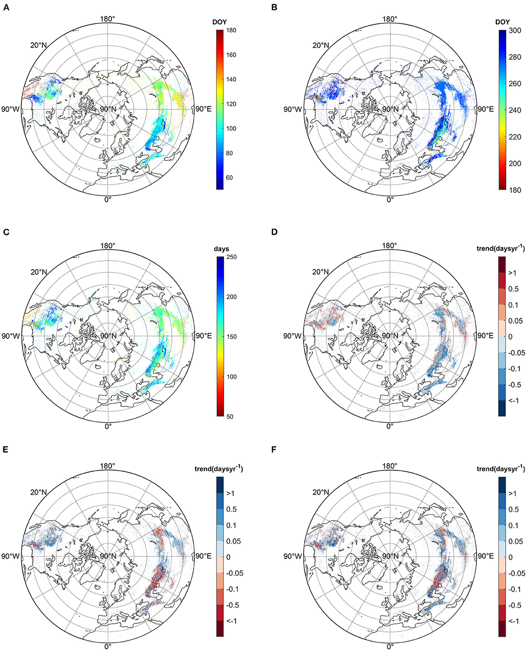
Figure 1. Annual mean SOS (A), EOS (B), GSL (C), and trends of SOS (D), EOS (E), and GSL (F) during the period of 1982–2011.

Grassland dormancy onset in the northern hemisphere primarily occurred between DOY 200 and 300 (Figure 1B), and around DOY 270 in East Asia. For Central Asia and Europe, the grassland dormancy occurred around DOY 280 and 230~250 in the regions of 50°N and between 40 and 50°N, respectively. EOS occurred later at lower latitude (lower than 40°N), around DOY 260–290. For the North American continent, most grasslands entered dormancy on DOY 280 or later, while a small proportion in the middle area of North America around 30°N experienced EOS between 200 and 250 in Julian day.

The mean GSL showed similar spatial patterns with EOS (Figure 1C). For Eurasia, grassland GSL ranged mainly between 140 and 230 days. For most parts of East Asia, grassland GSL lasted for almost 5 months, while in Central Asia it exhibited a little longer activity than in East Asia. GSL ranged between 180 and 230 days in the area of 50°N, while it was shortened to 140–170 days in the regions lower than 50°N. For Europe, grasslands remained active over 6 months (>180 days). Grassland GSL exhibited high spatial heterogeneities in North America. In the low latitudes, most grasslands exhibited a GSL between 100 and 150 days. In the northward latitudes, between 35 and 55°N, the GSL decreased to the range between 160 and 210 days. The growing season lasted for ~150 days in the middle NA and it was lengthened to ~210 days westward to the west coast.

Along the temporal dimension, grassland green-up advanced in nearly 65% of the studied grasslands, and 35% showed delayed trends (Figure 1D). In regions where GSL advanced, about 31% were significant (P < 0.05), while 19% of the delayed regions were significant. Spatially, 70 and 30% of Eurasia's grasslands exhibited advanced and delayed green-up, respectively. Advancement in green-up primarily concentrated in mid-latitude areas of central Asia and Europe. The fastest advances occurred northwest of the Caspian sea, with a value of −0.5 to −1 days/year. In the high latitude region of East Asia, grassland around 65°N displayed an advancing trend, and in the lower latitudes around 40°N of North China, grassland spring green-up onset also showed earlier variation. However, advancing shifts were slower than in central Asia, with a trend between −0.1 and −0.5 days/year. The delayed phenological trend was primarily found in the mid-latitudes of east Asia (mostly between 0.05 and 0.5 days/year), western Tibetan Plateau (primarily between 0.1 and 0.5 days/year), and high-latitude regions of central Asia and east Europe (<0.5 days/year). On the opposite, regions with a delayed trend in North America were slightly larger than those with advanced trend (51 vs. 49%). The delay occurred extensively over northern America and its magnitude abated from high latitudes (more than 1 day/year) to low latitudes (0.1 days/year). Nevertheless, advancing trends mainly concentrated on the northeast part of the grassland area (−0.5 to −0.1 days/year) over North America.

In terms of autumn dormancy (Figure 1E), more than 58% of the northern grasslands demonstrated delayed trends and nearly 22% of them reached significant levels (P < 0.05). Forty-two percent of the northern grasslands showed an advanced dormancy trend, with 13% of them being significant. Unlike spring phenology, the autumn dormancy trend displayed a clear clustered spatial pattern. In Eurasia, 46% of the grasslands indicated advancing trends and 54% showed delayed trend. In regions of East Asia between 40 and 50°N, grassland dormancy exhibited a prevailed delay during the past 30 years, with a trend between −0.5 and −0.1 days/year. In the southern part of East Asia, the delaying trend dominantly changed between 0.1 and 0.5 days/year over central China, and it decreased to <0.1 days/year south forward to the Tibetan Plateau. Westwards, grassland dormancy advanced by ~0.5 days/year on the east edge of Central Asia. However, the EOS trend advanced from east to west. In this area, the advancing trend around 50°N were mainly between −0.5 and −0.1 days/year, while the magnitude of the advancement increased southward around 45°N (>-0.5 days/year). In the western part of Eurasia, grasslands EOS trend shifted from advancing to delay westwards. In North America, delayed EOS accounted for 71% of grassland areas, and the trend slope decreased from low to high latitude. The EOS advancing was primarily concentrated in the west edge (−1 to −0.1 days/year) and the middle east part of NA grassland (~-1days/year).

The spatial pattern of the GSL trend was analogous to that of the EOS trend (Figure 1F). Sixty-four percent of the northern grassland areas showed extended growing seasons, and the remaining 36% displayed shortened ones. Spatially over Eurasia, 63% pixels indicated an extension trend and only 37% pixels showed a shortened trend. In East Asia between 40 and 50°N, grassland GSL primarily shortened with a rate between −0.5 and−0.1 days/year. However, in the south part of East Asia, grassland GSL extended by about 0.1 days/year. In the western Tibetan Plateau, alpine grassland GSL slightly shortened. From west of East Asia to Central Asia, GSL primarily extended with a rate between 0.1 and 1 days/year. The GSL trend in the middle region of Central Asia showed high heterogeneities, with a prevailing shortened GSL and the greatest magnitude in the eastern part of Kazakhstan (< -1 days/year). Westward to the northern Caspian Sea, grassland GSL showed an extended trend with a rate exceeding 0.5 days/year. In the relatively lower latitude area between 20 and 35°N of Central Asia and Europe, the GSL showed an extended trend between 0.1 and 0.5 days/year. Similar to Eurasia, in North America 65% of the area exhibited extended GSL and 35% exhibited shortened GSL. The regions with the most concentrated pattern of extended GSL trend were in the east part of North America between 40 and 50°N, with a rate >0.1 days/year. The shortened GSL trend was concentrated in the east part of North America grassland between 30 and 35°N (< -0.5 days/year).

Phenological Variations and Effects on GSL

The CV of SOS was the lowest among the three phenophases (Figure 2A). For Eurasia, CV was <0.05 in East Asia and high latitudes of Central Asia (around 50°N), while in middle and low latitudes of Central Asia and Europe, CV was larger (0.05–0.1). In North America, CV decreased latitudinally from 0.15 to 0.00 (Figure 2B). CV of EOS was slightly higher than that of SOS. In Eurasia, CV of East Asia was the smallest throughout the NH grassland (<0.05). For Central Asia, CV ranged between 0.05 and 0.10 in the regions around 50°N. Southwards, there was a belt with large EOS fluctuations (>0.15) between 45 and 50°N. In the lower latitude, CV decreased to about 0.07. In North America, CV in lower latitude mostly exceeded 0.15, and then decreased with latitude. Furthermore, in the high latitude regions between 35 and 50°N, CV in the east part (<0.05) was slightly higher than in the west part (0.05–0.10).

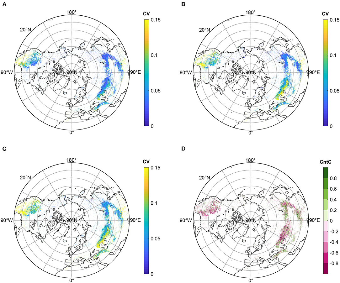
Figure 2. Coefficient of Variance (CV) of SOS (A), EOS (B), and GSL (C) during 1982–2012; Contribution coefficient (CntC) (D).

The spatial pattern of GSL CV was similar to that of EOS (Figure 2C). In Eurasia, the CV of East Asia grasslands were also the lowest, with an approximate value of 0.05. Similar to EOS CV, values in high latitude zones of Central Asia were about 0.08, and the belt in the lower latitudes of Central Asia also exhibited the highest CV (>0.15). Nevertheless, most parts of North America had high CV values, except its northeastern part exhibiting low values between 0.05 and 0.10.

To discriminate the respective effects of SOS and EOS, we further calculated CntC (Figure 2D). Areas with negative and positive values accounted for 55 and 45% of the NH grassland, respectively. Fifty-two and forty-eight percent of areas in Eurasia showed negative and positive CntC, respectively. In East Asia, the high latitude region (>45°N) primarily showed positive CntC between 0.00 and 0.80. Additionally, the low latitude area of the Tibetan Plateau also displayed positive CntC between 0 and 1. However, most regions in the middle latitude of East Asia indicated negative CntC, and the peak value (0.80–1.00) was found around 40°N. A majority of pixels in Central Asia north of 40°N possessed negative CntC, except the west part north of the Caspian Sea. The low negative CntC values were mainly distributed around 60°E. Areas south of 40°N of Central Asia and Europe primarily featured positive CntC, which were generally <0.80. In 64% of North American grasslands, CntC was negative and they did not show any zonation. Thirty-six percent of North America grasslands exhibited positive CntC and were sporadically distributed.

Factors Regulating Grassland Phenology

The driving factors analysis revealed that SOS dynamics were dominantly controlled by the interaction of temperature and precipitation or by temperature alone in 36% of the northern grasslands, while the SOS dynamics of the remaining 64% of the grasslands were controlled by other factors (Figure 3A). Advanced SOS was caused by the interactions of temperature and precipitation for 16% grassland. Temperature was the secondary dominant factor causing SOS to advance, predominating over 11% of the northern grasslands. Other climatic effects rarely emerged as dominant drivers of SOS temporal changes.

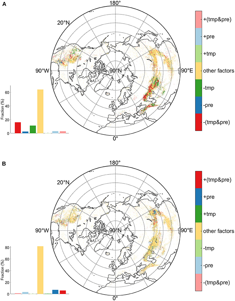
Figure 3. The primary effects on SOS (A) and EOS (B). The influencing factors includes temperature (tmp), precipitation (pre), the interaction of tmp and pre (tmp&pre), and other factors.

Spatially, SOS in East Asia was primarily controlled by other factors and their random interactions with temperature or precipitation. SOS of grassland in Central Asia and Europe was mainly driven by temperature and precipitation. Among them, temperature dominated areas were mainly concentrated in the east part of Central Asia, while the interaction of temperature and precipitation turned to be the primary driver westward. In North America, dominance by temperature, precipitation, or their interactions were found in different regions. In high latitude area, temperature advanced SOS in west part, while dominant effects from the interactions of temperature and precipitation were primarily found in the eastern portions. Advances in SOS caused by precipitation occurred in the southern NA grasslands.

EOS variations were dominantly regulated by other factors, as exhibited by its distribution in nearly 82% of the northern grasslands (Figure 3B). Unlike effects of climate factors on SOS, precipitation was the primary driver for the EOS delay (7% pixels), followed by the interaction of temperature and precipitation (6% pixels). Temperature effects regulated the least areas of EOS change. Spatially, delaying effects on EOS from precipitation were mainly concentrated in the eastern part of East Asia, and some small patches in the middle-high latitudes of Central Asia and North America. Interactions between temperature and precipitation were mainly found at high latitudes of East Asia and low latitudes of North America.

In order to get a more intuitive understanding on the influencing magnitude of factors on spring and autumn phenology, we identified the main factor of each pixel along the GSL gradient (Figure 4). Climatic effects on SOS and EOS displayed a divergent pattern along the GSL gradient. Climatic effects enhanced with extended GSL on SOS. Effects of the interactions between temperature and precipitation are obvious, while the temperature effect gradually emerges to be dominant in long GSL grasslands. Climatic factors explained a tiny fraction of EOS variations (Figure 4B). We further zoomed in Figure 4B in the part between 0.00 and 0.15% of the y-axis, in order to show the climatic control part, and explored how climatic factors influence the EOS fluxes (Figure 4C). There was no significant GSL trend, but precipitation was the most important climatic factor on grassland EOS.

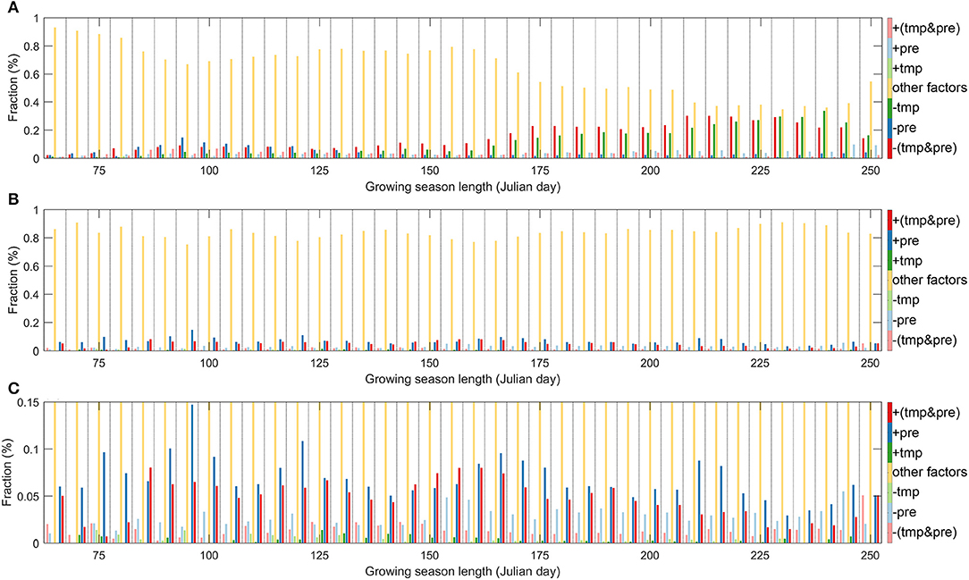
Figure 4. The effect factors of SOS (A) and EOS (B) on growing season length, and the magnified climatic effects in EOS (C).

Discussion

Spatial and Temporal Patterns of Grassland Phenology

In accordance with prior relevant studies, we identified an abnormal latitudinal SOS pattern in east Asia, where the Tibetan Plateau creates a regional elevation pattern (Piao et al., 2011; Cong et al., 2012). Exceptionally early SOS also occurs in northwest China (Cong et al., 2012), where early spring ephemeral plants have low temperature requirements (Wang et al., 2005). The alpine grasslands with relatively short GSL on the Tibetan Plateau displayed synchronous advanced SOS and EOS in response to climate change (Cong et al., 2017). Similar phenomena were also found for Central Asia grasslands (40–50°N). Precipitation is the primary limiting factor on vegetation phenology in Central Asia (Gessner et al., 2013). In these two regions, climate affect grassland phenology through similar mechanisms, by which plants deplete nutrients during the short growing season and then exhibit a low sensitivity to climate (Cong et al., 2017).

The NH grasslands exhibited a prevailing advanced green-up onset, especially in Eurasia, which was caused primarily by rising spring temperature (Supplementary Figure 1A). Eurasia has significantly warmed during the past three decades, while temperature exhibited a flat trend in North America. Increased spring temperature might favor advanced grassland green-up. However, EOS displayed an advanced pattern in response to elevated growing season temperature over the high latitude in Eurasia (Figure 1E and Supplementary Figure 1C). The opposite response pattern reveals that the EOS trend is regulated by complex factors other than sole temperature.

Compared with boreal forests, grasslands showed greater advances in SOS (Cong and Shen, 2016) and higher sensitivity to climate change. As boreal forests are composed of perennial woody plants and feature a much greater above-ground biomass than grasslands, forest ecosystems generally possess stronger resilience to external environmental fluctuations (Granier et al., 2000; Li et al., 2019). However, the EOS of boreal forests showed an even more prolonged delay than northern temperate grasslands, which further supports that more complicated driving forces act on EOS than on SOS. Additional confounding environmental factors can possibly affect plant dormancy, especially in the case of herbs. For instance, strong winds or frosts during late autumn could suddenly inhibit grassland activity. However, woody plants generally exhibit higher resistance to extreme climate events. We can conclude that driving forces on grassland EOS contain other uncertainties beyond climate regulations.

Contributions of SOS and EOS to GSL Variation

We can detect the similarity between SOS/EOS and GSL by comparing their CVs. The low CV value suggests relatively stable variation of the phenology time series. SOS CV shows slight fluctuation and indicates that SOS is probably controlled by simple drivers. Our result indirectly confirms the previous studies that spring phenology is primarily driven by early spring temperature in the recent decades (Piao et al., 2006; Jeong et al., 2011). EOS CV shows larger fluctuation in comparison with SOS, indicating more complicated mechanism. In agreement with previous studies, vegetation autumn phenology is controlled by even more elements except for temperature (Barichivich et al., 2013). And the dynamic of EOS series fluctuated with the interaction of many factors under global warming. The CV pattern of GSL indicates similarity with EOS, and it is possibly implied that EOS dominantly determine the dynamic of GSL. Therefore, we need further analysis to quantitatively explore the contribution of EOS to GSL variation.

Piao et al. (2008) indicated that GPP increase exceeded that of respiration over the NH under early spring warming, but the difference reversed under autumn warming. Therefore, although an extension in GSL could add to GPP accumulation in most cases, a change in EOS probably cannot increase the carbon sink. The GSL variations showed higher consistency with EOS than with SOS. In further detecting the regulation of CntC on GSL, we rearranged the pixels in another dimension. Figure 5 shows the CntC and phenology trends along vegetation GSL. We can see the NH grassland GSL ranged between 125 and 225 days (Figure 5C). The value of CntC turned from positive to negative along the extended GSL (Figure 5A). This indicates apparent effects of EOS variations on the GSL in regions with relatively long vegetation growing season and the effects further enhanced with extended GSL, and this pattern was further confirmed by phenology trends along GSL gradient (Figures 5A,B). Along an extended GSL, the SOS maintained a flat trend, while EOS exhibited a significantly delayed trend. Plants with short GSL must finish their life rhythm in the short active period, while those with long GSL possess adequate response time in facing changes in climate (Cong et al., 2017). Therefore, delayed EOS in response to warming mostly occurred in ecosystems with long GSL. This finding further indicates the complexity of EOS variations and their driving forces.

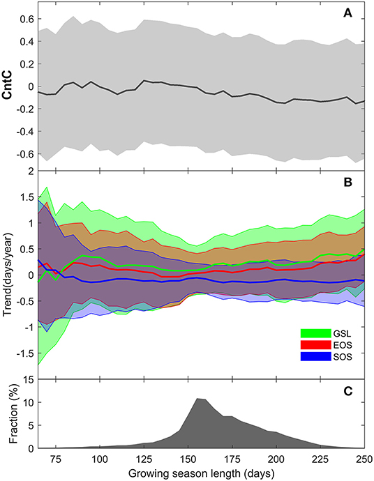
Figure 5. CntC (A) and phenology trends (B) along growing season length (C).

Analyses on Drivers for Different Phenophases

Vegetation SOS and EOS are regulated by complicated biological and environmental factors. Previous studies have been mostly focused on climate effects on vegetation spring green-up (Piao et al., 2006; Cong et al., 2013). However, driving forces on phenology are diverse. In arid and semi-arid areas, vegetation activity is closely linked with moisture thorough their growing periods (Kariyeva et al., 2012), but its interactions with temperature also plays a significant role. Seeds endure severe winter and green up in early spring highly depend on hydrothermal condition (Cong et al., 2013). Therefore, vegetation activity interactions with temperature set a key threshold rather than their sole effect. To be noted, grassland ecosystem is a complex synthesis, and the activity is driven by many “other factors” besides temperature and precipitation. Some internal and external factors have been proved to show influence on EOS in previous studies. For instance, Cong et al. (2017) found earlier SOS could advance EOS in southwest of Tibetan Plateau. Extreme events such as coldness or hotness could also affect the trend of EOS (Estrella and Menzel, 2006; Xie et al., 2015). We do not add more influencing factor data in this study because of lack of valid dataset at hemisphere scale. Additionally, we tried this new analytical method for the first time and we would improve this formula with more variables at regional scale in our future study.

Climate regulation effects on phenology varied with GSL (Figure 5). For example, alpine grasslands on the Tibetan Plateau exhibited a pattern of being less sensitive to climate change for those grasslands with shorter growing season (Cong et al., 2017). For grasslands with longer GSL, the positive effects from climates on vegetation phenology dominate. However, grassland GSL would not continuously extend under predicted global warming. On one hand, precipitation has maintained a flat trend as temperature kept increasing during the past three decades. The effects of the interactions between temperature and precipitation on phenology underscore their mutual regulation. However, precipitation probably cannot keep the pace with additional moisture requirements created by increased temperature. On the other hand, GSL is co-determined by SOS and EOS, which are rarely controlled by the same set of climatic factors. Here, we define the same climatic factor is that the grassland pixel is controlled by the same form of climate. For example, for one grassland pixel, its SOS is advanced by increase of early spring temperature, and EOS is delayed by increase of autumn temperature. The GSL extension is thus driven by temperature increase, and we consider the dynamic of phenology on this pixel is controlled by the same climatic factor. We further investigated the common climatic regulation factors on SOS and EOS (Supplementary Figure 2). For a tiny fraction of the N.H. grasslands, their SOS and EOS are controlled by common climatic factors, where their interaction play a dominant role. Temperature and precipitation need to reach a balance in creating optimal conditions for vegetation growth, while this balance is hard to achieve under climate fluctuations. Due to the antagonism interactions among each climate factor and environmental factors, grassland GSL extension would face a mounting inhibiting regulation under global warming.

Conclusion

In this study, we analyzed grassland phenology north of 30°N with multiple remote sensing methods. SOS shows clear spatial patterns in comparison with EOS. However, GSL dynamics is primarily controlled by EOS changes. Long term SOS series respond sensitively to climate change, and the interaction of temperature and precipitation is the dominant effect, followed by temperature. Only a small proportion of EOS pixels are driven by climate factors, while precipitation is the dominant driver among these pixels. For most grasslands, EOS is mainly regulated by other factors, which means that EOS dynamics is driven by complicated mechanisms even though significant global warming occurred over the NH. The unsynchronized driving mechanism on the dynamics of spring and autumn phenology probably determines that the GSL cannot extend without limits. Grassland ecosystems respond to climate change and resist environmental change via internal regulation. The complicated driving mechanisms on EOS and SOS imply that grassland phenology could self-regulate despite being sensitive to climate change. The complicated “other factors” are important for future studies to test the dominant driver of EOS and the interaction of affecting factors. Separating the other factors in regional scale or in situ experiment is primarily concerned in our future study.

Data Availability Statement

The original contributions presented in the study are included in the article/Supplementary Materials, further inquiries can be directed to the corresponding author/s.

Author Contributions

NC and YZ designed research. NC performed research. NC and KH provided measurements. NC, KH, and YZ wrote the paper. All authors contributed to the article and approved the submitted version.

Funding

This study was supported by the National Key Research & Development Program (2018YFA0606101 and 2019YFA0607302), the National Natural Science Foundation of China (Grant Nos. 42071133, 41991234, and 41725003).

Conflict of Interest

The authors declare that the research was conducted in the absence of any commercial or financial relationships that could be construed as a potential conflict of interest.

Supplementary Material

The Supplementary Material for this article can be found online at: https://www.frontiersin.org/articles/10.3389/ffgc.2020.610162/full#supplementary-material

Supplementary Figure 1. Trends of spring temperature (A), spring precipitation (B), autumn temperature (C), and autumn precipitation (D) from 1982 to 2011.

Supplementary Figure 2. The same climatic factors on SOS and EOS. The area with gray color is the continent, and only a tiny colored pixels indicate the same affecting climatic factor.

References

Barichivich, J., Briffa, K. R., Myneni, R. B., Osborn, T. J., Melvin, T. M., Ciais, P., et al. (2013). Large-scale variations in the vegetation growing season and annual cycle of atmospheric CO2 at high northern latitudes from 1950 to 2011. Glob. Chang. Biol. 19, 3167–3183. doi: 10.1111/gcb.12283
Borcard, D. F. G., and Legendre, P. (2010). Numerical Ecology in R. New York, NY: Springer, 180–182. doi: 10.1007/978-1-4419-7976-6
Choler, P. (2015). Growth response of temperate mountain grasslands to inter-annual variations in snow cover duration. Biogeosciences 12, 3885–3897. doi: 10.5194/bg-12-3885-2015
Cong, N., Piao, S., Chen, A., Wang, X., Lin, X., Chen, S., et al. (2012). Spring vegetation green-up date in China inferred from SPOT NDVI data: a multiple model analysis. Agric. For. Meteorol. 165, 104–113. doi: 10.1016/j.agrformet.2012.06.009
Cong, N., and Shen, M. (2016). Variation of satellite-based spring vegetation phenology and the relationship with climate in the northern hemisphere over 1982 to 2009. Chin. J. Appl. Ecol. 27, 2737–2746. doi: 10.13287/j.1001-9332.201609.028
Cong, N., Shen, M., Piao, S., and Piao, S. (2017). Spatial variations in responses of vegetation autumn phenology to climate change on the tibetan plateau. J. Plant Ecol. 10, 744–752. doi: 10.1093/jpe/rtw084
Cong, N., Wang, T., Nan, H., Ma, Y., Wang, X., Myneni, R. B., et al. (2013). Changes in satellite-derived spring vegetation green-up date and its linkage to climate in China from 1982 to 2010: a multi-method analysis. Glob. Chang. Biol. 19, 887–891. doi: 10.1111/gcb.12077
Ellis, E. C., and Ramankutty, N. (2008). Putting people in the map: anthropogenic biomes of the world. Front. Ecol. Environment. 6, 439–447. doi: 10.1890/070062
Estiarte, M., and Peñuelas, J. (2015). Alteration of the phenology of leaf senescence and fall in winter deciduous species by climate change: effects on nutrient proficiency. Glob. Chang. Biol. 21, 1005–1017. doi: 10.1111/gcb.12804
Estrella, N., and Menzel, A. (2006). Responses of leaf colouring in four deciduous tree species to climate and weather in Germany. Clim. Res. 32, 253–267. doi: 10.3354/cr032253
Fu, Y., Piao, S., Zhao, H., Jeong, S. J., Wang, X., Vitasse, Y., et al. (2014). Unexpected role of winter precipitation in determining heat requirement for spring vegetation green-up at northern middle and high latitudes. Glob. Chang. Biol. 20, 3743–3755. doi: 10.1111/gcb.12610
Fu, Y., Zhang, X., Piao, S., Hao, F., Geng, X., Vitasse, Y., et al. (2019). Daylength helps temperate deciduous trees to leaf-out at the optimal time. Glob. Chang. Biol. 25, 2410–2418. doi: 10.1111/gcb.14633
Garonna, I., deJong, R., deWit, A., Mücher, C. A., Schmid, B., and Schaepman, M. E. (2014). Strong contribution of autumn phenology to changes in satellite-derived growing season length estimates across Europe (1982-2011). Glob. Chang. Biol. 20, 3457–3470. doi: 10.1111/gcb.12625
Gessner, U., Naeimi, V., Klein, I., Kuenzer, C., Klein, D., and Dech, S. (2013). The relationship between precipitation anomalies and satellite-derived vegetation activity in Central Asia. Glob. Planet. Change 110, 74–87 doi: 10.1016/j.gloplacha.2012.09.007
Granier, A., Biron, P., and Lemoine, D. (2000). Water balance, transpiration and canopy conductance in two beech stands. Agric. For. Meteorol. 100, 291–308. doi: 10.1016/S0168-1923(99)00151-3
Hu, H., Boisson-Dernier, A., Israelsson-Nordstöm, M., Böhmer, M., Xue, S., Ries, A., et al. (2011). Carbonic anhydrases are upstream regulators of CO2-controlled stomatal movements in guard cells. Nat. Cell Biol. 12, 87–93. doi: 10.1038/ncb2009
Jeong, S. J., Ho, C. H., Gim, H. J., and Brown, M. E. (2011). Phenology shifts at start vs. end of growing season in temperate vegetation over the northern hemisphere for the period 1982-2008. Glob. Chang. Biol. 17, 2385–2399. doi: 10.1111/j.1365-2486.2011.02397.x
Kariyeva, J., van Leeuwen, W. J. D., and Woodhouse, C. A. (2012). Impacts of climate gradients on the vegetation phenology of major land use types in Central Asia (1981–2008). Front. Earth Sci. 6, 206–225. doi: 10.1007/s11707-012-0315-1
Keeling, R., Piper, S., and Heimann, M. (1996). Global and hemispheric CO2 sinks deduced from changes in atmospheric O2 concentration. Nature 381, 218–221. doi: 10.1038/381218a0
Keskitalo, J., Bergquist, G., Gardeström, P., and Jansson, S. (2005). A cellular timetable of autumn senescence. Plant Physiol. 139, 1635–1648. doi: 10.1104/pp.105.066845
Knapp, A., and Smith, M. (2001). Variation among biomes in temporal dynamics of aboveground primary production. Science 291:481. doi: 10.1126/science.291.5503.481
Körner, C., and Basler, D. (2010). Phenology under global warming. Science 327, 1461–1462. doi: 10.1126/science.1186473
Kraha, A., Turner, H., Nimon, K., Zientek, L., and Henson, R. K. (2012). Tools to support interpreting multiple regression in the face of multicollinearity. Front. Psychol. 3:44. doi: 10.3389/fpsyg.2012.00044
Lebreton, J. M., Ployhart, R. E., and Ladd, R. T. (2004). A monte carlo comparison of relative importance methodologies. Organ. Res. Methods 7, 258–282. doi: 10.1177/1094428104266017
Li, J., Cong, N., Zu, J., Xin, Y., Huang, K., Zhou, Q., et al. (2019). Longer conserved alpine forests ecosystem exhibits higher stability to climate change on the tibetan plateau. J. Plant Ecol. 12, 645–652. doi: 10.1093/jpe/rtz001
Liu, Q., Fu, Y., Zhu, Z., Liu, Y., Liu, Z., Huang, M., et al. (2016). Delayed autumn phenology in the northern hemisphere is related to change in both climate and spring phenology. Glob. Chang. Biol. 22, 3702–3711. doi: 10.1111/gcb.13311
Lucht, W., Prentice, I. C., Myneni, R. B., Sitch, S., Friedlingstein, P., Cramer, W., et al. (2002). Climatic control of the high-latitude vegetation greening trend and pinatubo effect. Science 296, 1687–1689. doi: 10.1126/science.1071828
Marchin, R. M., Salk, C. F., Hoffmann, W. A., and Dunn, R. R. (2015). Temperature alone does not explain phenological variation of diverse temperate plants under experimental warming. Glob. Chang. Biol. 21, 3138–3151. doi: 10.1111/gcb.12919
Menzel, A., and Fabian, P. (1999). Growing season extended in Europe. Nature 397:659. doi: 10.1038/17709
Menzel, A., Sparks, T. H., Estrella, N., Koch, E., Aasa, A., Ahas, R., et al. (2006). European phenological response to climate change matches the warming pattern. Glob. Chang. Biol. 12, 1969–1976. doi: 10.1111/j.1365-2486.2006.01193.x
Myneni, R. B., Keeling, C. D., Tucker, C. J., Asrar, G., and Nemani, R. R. (1997). Increased plant growth in the northern high latitudes from 1981 to 1991. Nature 386, 698–702. doi: 10.1038/386698a0
New, M., Hulme, M., and Jones, P. (2000). Representing twentieth-century space-time climate variability. Part II: development of 1901-96 monthly grids of terrestrial surface climate. Am. Meteorol. Soc. 13, 2217–2238. doi: 10.1175/1520-0442(2000)013<2217:RTCSTC>2.0.CO;2
New, M., Lister, D., Hulme, M., and Makin, I. (2002). A high-resolution data set of surface climate over global land areas. Clim. Res. 21, 2–25. doi: 10.3354/cr021001
Parmesan, C. (2007). Influences of species, latitudes and methodologies on estimates of phenological response to gloval warming. Glob. Chang. Biol. 13, 1860–1872. doi: 10.1111/j.1365-2486.2007.01404.x
Piao, S., Ciais, P., Friedlingstein, P., Peylin, P., Reichstein, M., Luyssaert, S., et al. (2008). Net carbon dioxide losses of northern ecosystems in response to autumn warming. Nature 451, 49–53. doi: 10.1038/nature06444
Piao, S., Cui, M., Chen, A., Wang, X., Ciais, P., Liu, J., et al. (2011). Altitude and temperature dependence of change in the spring vegetation green-up date from 1982 to 2006 in the qinghai-xizang plateau. Agric. For. Meteorol. 151, 1599–1608. doi: 10.1016/j.agrformet.2011.06.016
Piao, S., Fang, J., Zhou, L., Ciais, P., and Zhu, B. (2006). Variations in satellite-derived phenology in China's temperate vegetation. Glob. Chang. Biol. 12, 672–685. doi: 10.1111/j.1365-2486.2006.01123.x
Piao, S., Liu, Q., Chen, A., Jassens, I. A., Fu, Y., Dai, J., et al. (2019). Plant phenology and global climate change: current progresses and challenges. Glob. Chang. Biol. 25, 1922–1940. doi: 10.1111/gcb.14619
Piao, S., Liu, Z., Wang, T., Peng, S., and Tans, P. P. (2017). Weakening temperature control on the interannual variations of spring carbon uptake across northern lands. Nat. Clim. Change 7, 359–363. doi: 10.1038/nclimate3277
Piao, S., Wang, X., Park, T., Chen, C., and Myneni, R. (2020). Characteristics, drivers and feedbacks of global greening. Nat. Rev. Earth Environ. 1, 14–27. doi: 10.1038/s43017-019-0001-x
Schwartz, M., Ahas, R., and Aasa, A. (2006). Onset of spring starting earlier across the Northern hemisphere. Glob. Chang. Biol. 12, 343–351. doi: 10.1111/j.1365-2486.2005.01097.x
Shen, M., Piao, S., Cong, N., Zhang, G., and Jassens, I. A. (2015). Precipitation impacts on vegetation spring phenology on the tibetan plateau. Glob. Chang. Biol. 21, 3647–3656. doi: 10.1111/gcb.12961
Shen, M., Tang, Y., Chen, J., Yang, X., Wang, C., Cui, X., et al. (2014). Earlier-season vegetation has greater temperature sensitivity of spring phenology in northern hemisphere. PLoS ONE 9:e88178. doi: 10.1371/journal.pone.0088178
Tucker, C., Pinzon, J., Brown, M., Slayback, D., Pak, E., Mahoney, R., et al. (2005). An extended AVHRR 8-km NDVI dataset compatible with MODIS and SPOT vegetation NDVI data. Int. J. Remote Sens. 26, 4485–4498. doi: 10.1080/01431160500168686
Wang, H., Li, X., Li, X. B., Yu, F., Yu, H., and Yang, H. (2005). The correlation between meteorological factors and NDVI in Northeastern China. J. Beijing Normal Univ. 41, 425–430. doi: 10.1007/s10409-004-0010-x
Wang, X., Wang, T., Guo, H., Liu, D., Zhao, Y., Zhang, T., et al. (2017). Disentangling the mechanisms behind winter snow impact on vegetation activity in northern ecosystems. Glob. Chang. Biol. 24, 1651–1662. doi: 10.1111/gcb.13930
Way, D. A., and Montgomery, R. A. (2015). Photoperiod constraints on tree phenology, performance and migration in a warming world. Plant Cell Environ. 38, 1725–1736. doi: 10.1111/pce.12431
Weltzin, J., Lolk, M., Schwinning, S., Williams, D. G., Fay, P. A., Haddad, B. M., et al. (2003). Assessing the response of terrestrial ecosystems to potential changes in precipitation. BioScience 53, 941–952. doi: 10.1641/0006-3568(2003)053[0941:ATROTE]2.0.CO;2
White, M. A., deBeurs, K. M., Didan, K., Inouye, D. W., Richardson, A. D., Jensen, O. P., et al. (2009). Intercomparison, interpretation, and assessment of spring phenology in North America estimated from remote sensing for 1982-2006. Glob. Chang. Biol. 15, 2335–2359. doi: 10.1111/j.1365-2486.2009.01910.x
White, M. A., Hoffman, F. M., Hargove, W., and Nemani, R. (2005). A global framework for monitoring phenological responses to climate change. Geophys. Res. Lett. 32:L04705. doi: 10.1029/2004GL021961
Xie, Y., Wang, X., and Silander, J. (2015). Deciduous forest responses to temperature, precipitation, and drought imply complex climate change impacts. Proc. Natl. Acad. Sci. U.S.A. 112, 13585–13590. doi: 10.1073/pnas.1509991112
Yang, Y., Guan, H., Shen, M., Liang, W., and Jiang, L. (2015). Changes in autumn vegetation dormancy onset date and the climate controls across temperate ecosystems in china from 1982 to 2010. Glob. Chang. Biol. 21, 652–665. doi: 10.1111/gcb.12778
Zeng, H. Q., Jia, G. S., and Epstein, H. (2011). Recent changes in phenology over the northern high latitudes detected from multi-satellite data. Environ. Res. Lett. 6:045508. doi: 10.1088/1748-9326/6/4/045508
Zhang, X., Friedl, M. A., Schaaf, C. B., and Strahler, A. H. (2004). Climate controls on vegetation phenological patterns in northern mid- and high latitudes inferred from MODIS data. Glob. Chang. Biol. 10, 1133–1145. doi: 10.1111/j.1529-8817.2003.00784.x
Zhang, X., Liu, L., and Henebry, G. M. (2019). Impacts of land cover and land use change on long-term trend of land surface phenology: a case study in agricultural ecosystems. Environ. Res. Lett. 14:044020. doi: 10.1088/1748-9326/ab04d2
Keywords: land surface phenology, grassland, growing season length, interaction of temperature and precipitation, multivariate relational model
Citation: Cong N, Huang K and Zhang Y (2021) Unsynchronized Driving Mechanisms of Spring and Autumn Phenology Over Northern Hemisphere Grasslands. Front. For. Glob. Change 3:610162. doi: 10.3389/ffgc.2020.610162
Received: 25 September 2020; Accepted: 30 November 2020;
Published: 20 January 2021.
Edited by:
Yongshuo Fu, Beijing Normal University, ChinaReviewed by:
Hongfang Zhao, East China Normal University, ChinaXuancheng Zhou, Beijing Normal University, China
Copyright © 2021 Cong, Huang and Zhang. This is an open-access article distributed under the terms of the Creative Commons Attribution License (CC BY). The use, distribution or reproduction in other forums is permitted, provided the original author(s) and the copyright owner(s) are credited and that the original publication in this journal is cited, in accordance with accepted academic practice. No use, distribution or reproduction is permitted which does not comply with these terms.
*Correspondence: Yangjian Zhang, zhangyj@igsnrr.ac.cn
†These authors have contributed equally to this work