Summer Distribution of Total Suspended Matter Across the Baltic Sea

Introduction

Marine waters are usually divided into optical case 1 and optical case 2 waters (Morel and Prieur, 1977). Optical case 1 waters are waters where the optical properties, are dominated by phytoplankton and co-varying colored dissolved organic matter (CDOM), besides the optical properties of water itself. Typical examples of case 1 waters are clear ocean waters, and the clearest water known is the Sargasso Sea (Kirk, 1985). Optical case 2 waters are coastal waters that are influenced by terrestrial run-off, and thus are optically also influenced by total suspended matter (TSM, also termed suspended particulate matter, SPM) and by CDOM. Baltic Sea waters are generally classified as optical case 2 waters with a relatively strong optical influence from CDOM (Kowalczuk et al., 2006; Kratzer and Tett, 2009; Kratzer and Moore, 2018). Many marine waters, however, are also strongly influenced by TSM, especially waters that have a strong tidal influence where the resuspension of sediments may reach much further off-shore than in the Baltic Sea. In some coastal areas, there is also a strong influence of TSM due to both high river run-off and tidal influence. Examples for this are the Thames Estuary where, according to Devlin et al. (2008) estuarine waters typically have much higher concentrations of TSM (8.2–73.8 gm⁻³) compared to coastal waters (3.0–24.1 gm⁻³). Off-shore waters showed concentrations of up to 9.3 gm⁻³ which is much higher than found in the Baltic Sea. Kratzer and Tett (2009), for example found that in summer (Western Gotland Basin) the measured TSM ranged from only 0.48–1.34 gm⁻³ in the open sea (n = 18) and 0.48–2.77 gm⁻³ in coastal areas (n = 22). Kratzer and Moore (2018) found a range of 0.44 gm⁻³-4.82 gm⁻³ in the open sea (n = 43) with a median of 1.00 gm⁻³ and 0.48–3.36 gm⁻³ in coastal areas (n = 55) with a median of 1.62 gm⁻³. High TSM values in the open sea were usually related to very high chl-a concentrations during the occurrence of cyanobacteria blooms in summer. Harvey (2015) and Harvey et al. (2018) measured ranges of 0.5–21.7 gm⁻³ in the W Gotland Basin by including areas with stronger terrestrial influence such as Bråviken and Nyköping bay. Table 1 gives an overview of TSM measured in situ in different sub-basins of the Baltic Sea. There are some areas in the world with much higher terrestrial influence. For example, the Rio de Plata at the border between Argentina and Uruguay has shown to have very high turbidity ranging from 62–185 NTU, and the Gironde Estuary in southwest France showed ranges of 41–988 FNU (Dogliotti et al., 2015).

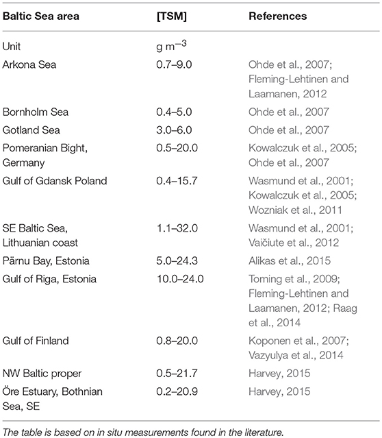
Table 1. Comparison of the ranges of TSM concentrations [TSM] in different sub-basins of the Baltic Sea.

In essence, it is the spectral absorption and scattering properties of each optical component that govern the underwater light field, and also the reflectance, i.e., the color of the sea that we can perceive, and that can also be measured remotely from space. Colored dissolved organic matter (CDOM) absorbs light, especially in the blue part of the visible spectrum. The absorption curve follows a logarithmic decline (Kirk, 1985). Because of the high absorption in the blue and green parts of the spectrum CDOM makes the water look more yellow—or even brown at very high CDOM concentrations. The strong absorption of CDOM also makes the water look darker as it reflects much less light. Inorganic suspended matter mostly scatters light, whereas organic suspended matter mostly absorbs light and behaves optically in a similar way to CDOM. Due to the strong scattering of light, inorganic suspended matter usually increases the brightness of a satellite image. Phytoplankton mostly absorbs light in the blue and in the red part of the spectrum due to the absorption of chlorophyll pigments. Carotenoid pigments also absorb in the blue-green and are usually correlated to chlorophyll-a. Phycobilin pigments are usually found in cyanobacteria and in the Baltic Sea, they tend to absorb light in the 560 and 620 nm region (Kratzer, 2000). CDOM originates mostly from terrestrial plants on land and usually indicates input of freshwater. Inorganic suspended matter indicates land drainage and wind-stirring in shallow waters (Kratzer and Tett, 2009). Total suspended matter (TSM) is strongly correlated to turbidity (Kari et al., 2017) which is a supportive parameter in the EU Marine Strategy Framework Directive Annex III (2008), especially in coastal waters. Phytoplankton is affected by anthropogenic nutrients from land and thus indicates the productive status of the pelagic ecosystem (Kratzer and Tett, 2009). Chl-a is often used as a proxy for phytoplankton biomass and an indicator for eutrophication.

In this study we focus on TSM as can be used as an indicator for the extent of coastal waters in a bio-optical model developed in the Baltic Sea. Kratzer and Tett (2009) used TSM to define the breadth of coastal waters using the inorganic fraction as an indicator. It was found that inorganic suspended matter tends toward zero at a distance of tens of kilometer from the shore. Inorganic suspended matter is also the optical component that showed a clear difference in distribution between inner coastal and open sea waters. The trendline showed a relatively steep decline in the inner Himmerfjärden bay, and off the cost with a much flatter trendline. All optical components were best described with a polynomial function when moving from the shore (source) to Landsort deep (sink) Kratzer and Tett (2009). This was explained due to the fact that the Baltic Sea has almost no tidal influence, making diffusion the main physical force for the distribution of particles. Also, the W Gotland Basin has relatively low influence from wind forcing when, for example, compared to the Southern Baltic Sea (Danielsson et al., 2007). The wind field has shown to have a strong effect on the resuspension patterns in the Baltic proper. Kuhrts et al. (2004) found that sediment transport is generally smaller in summer because of lower winds. In wintertime, the wind forcing is stronger and due to the vertical mixing and enhanced vertical current shear, the resuspension of sediment is stronger. The authors also found that the transport of sedimentary material over longer distances occurs only under extreme wind events that are relatively rare. There are several mechanisms that may induce currents in the Baltic Sea: wind stress at the sea surface, surface pressure gradients, thermohaline horizontal gradients of density, as well as tidal forces. All these currents are also influenced by Coriolis acceleration, as well as bottom topography and friction, forming a general (cyclonic) circulation in the stratified system (Myrberg and Lehmann, 2013), generating mesoscale eddies. These physical processes are often shown on satellite images depicting cyanobacteria blooms in the Baltic Sea (Kahru et al., 2007; Kratzer et al., 2011, 2014; Kahru and Elmgren, 2014). These processes may also carry suspended matter up to 150 km off-shore (Kyryliuk, 2014), especially in the Southern Baltic Sea.

HELCOM's Monitoring and Assessment Strategy

One of the Helsinki Commission's (HELCOM) Monitoring and Assessment Strategy objectives is “to facilitate the implementation of the ecosystem approach, covering the whole Baltic Sea, including coastal and open waters” and “to enable the provision of data and information that links pressures on land, from the atmosphere, in coastal areas and at sea to their impacts on the marine environment” (HELCOM, 2013). The HELCOM Strategy aims to provide assessment and monitoring of data that can be utilized for both international assessment by HELCOM as well as for monitoring on a national level. The strategy is designed in such a way that insures both data production and dissemination of information by the Contracting Parties of the EU Member States and fulfilling the requirements of several EU directives such as the Marine Strategy Framework Directive (MSFD), the Water Framework Directive (WFD), the Habitats and Birds Directives, the EU Strategy for the Baltic Sea Region (EUSBSR), and the EU Integrated Maritime Policy (HELCOM, 2013). Foremost, the Strategy is aimed to support ecosystem-based Maritime Spatial Planning (MSP) in the Baltic Sea by enabling high-quality spatial data and assessment tools for the purposes envisioned for MSP. This latter aim led to the formation of the idea to investigate whether the use of TSM data derived from MERIS can be used in the sense of MSP as a “high-quality spatial data” and as an assessment tool, covering the last assessment period of HELCOM.

For the purposes of regional assessment HELCOM sub-divides Baltic Sea into the different sub-basins. Those basins are described in the document “HELCOM sub-divisions of the Baltic Sea” (Attachment 4; HELCOM, 2013), following distinctive hierarchical levels of sub-division, depending on management needs. For the purposes of this study the sub-division of the Baltic Sea into 16 sub-basins is used (Table 2) in order to comply with general management practices in the Baltic Sea basin.

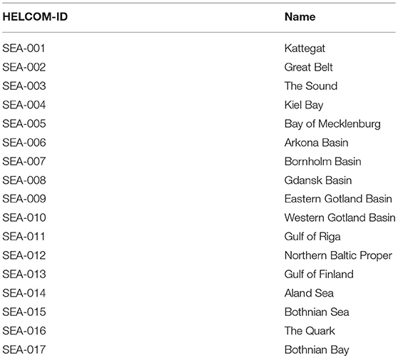
Table 2. Nomenclature of sub-basins of the Baltic Sea according to HELCOM.

Aims and Objectives

It is the aim of this study to (1) evaluate the difference in TSM loads in the different sub-basins of the Baltic Sea and to compare them statistically. In order to do this, data from the MEdium Resolution Imaging Spectrometer (MERIS with 300 m resolution) was used. MERIS was developed by the European Space Agency (ESA) and was launched on ENVISAT in early 2002 and operated until early 2012. The MERIS data was used to generate TSM composites of all viable MERIS scenes from summers 2009, 2011, and 2011. These yearly summer composites were then aggregated into a 3-year summer composite (2009–2011), which gives a seasonal overview of TSM distribution across the different Baltic Sea basins. This 3-year summer composite was then divided into the different HELCOM sub-basins for statistical comparison. Furthermore, it is the aim (2) to evaluate the differences in coastal distribution patterns along a transect reaching from the inner Himmerfjärden bay out into the open sea, thus covering a range of coastal to off-shore water types. As the distribution of TSM in the southwestern Baltic Sea is highly influenced by meso-scale eddies we focus here on a transect set in the W Gotland Basin. We also (3) discuss how the concentrations derived from MERIS data compare to in situ data found in the literature, and discuss the application of this approach in environmental monitoring and management of the Baltic Sea.

Materials and Methods

Area of Investigation

The Baltic Sea is a brackish ecosystem with many distinguishable characteristics, and is sometimes described as a large fjord-like estuary with brackish water, driven by river run-off, and weather conditions over the Baltic Sea-North Sea region (Kullenberg and Jacobsen, 1981; Voipio, 1981). The Baltic is, however, much larger and deeper than an average estuary and has narrow and shallow connections with the North Atlantic Ocean. In this respect, it would be more similar to a gigantic threshold fjord with a series of sub-basins (Snoeijs-Leijonmalm et al., 2017).

Overall, the Baltic Sea is characterized by a permanent halocline with higher saline waters in the bottom layers (originating from the North Sea), and brackish waters in the top layers. High fluvial input to the surface layers creates a strong north-south facing horizontal salinity gradient across the Baltic Sea basin. For example, the salinity is about 3–2 g kg⁻¹ in the Bothnian Bay, and about 8–6 g kg⁻¹ in the Baltic Proper. The Baltic Sea topography is divided into a series of basins separated by shallow areas, and has a mean depth of 56 m, where nearly 17% of the area are no more than 10 m deep (Kullenberg and Jacobsen, 1981). With 459 m depth, Landsort Deep in the NW Baltic proper is the deepest part of the Baltic Sea. The main circulation in the Baltic Sea is driven by wind and deviations in atmospheric pressure (Leppäranta and Myrberg, 2009). The Northern Baltic is dominated by Precambrian and Paleozoic bed rock whilst the Southern areas of the Baltic Sea bottoms consist mostly of alluvial sediments (Kullenberg and Jacobsen, 1981). Large amounts of river discharge, especially in the Southern Baltic bring in high levels of humic substances and suspended matter, which from an ocean color point of view, makes the Baltic Sea comprise optical case 2 waters, i.e., waters that, besides being optically dominated by phytoplankton may also contain large amounts of TSM and CDOM (Kratzer et al., 2003; Harvey, 2015; Kopelevich et al., 2016).

Himmerfjärden (HF) is a north-south facing, elongated bay located in the Northern Baltic Proper about 60 km south of Stockholm, Sweden (Engqvist, 1996) (Figure 1). HF is optically dominated by the absorption of CDOM (g440) ranging from 0.3–1.2 m⁻¹ (Kratzer and Moore, 2018) and TSM load ranges from 0.5–2.7 gm⁻³ with a polynomial gradient toward the open sea (Kratzer and Tett, 2009). Himmerfjärden receives a relatively minor freshwater input from lake Mälaren, however it is also under strong influence from the third largest sewage treatment plant in the Stockholm region (Franzén et al., 2011). The bay has been extensively studied for over 30 years and is regularly monitored by the Marine Monitoring Group at Stockholm University (SU) and since the late 90s also investigated by the Marine Remote Sensing Group (SU), combining dedicated optical campaigns with satellite data (e.g., Envisat/MERIS, Sentinel-2/MSI, and Sentinel-3/OLCI).

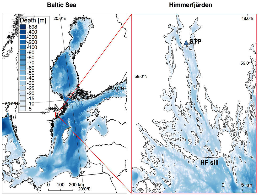
Figure 1. Area of investigation. Baltic Sea and Himmerfjaäden bay (HF), Swedish coastal areas. STP: Sewage Treatment Plant. Bathymetry data (Shom, 2018); (http://portal.emodnet-bathymetry.eu/). European coastline shapefile (European Environment Agency; https://www.eea.europa.eu/ds_resolveuid/06227e40310045408ac8be0d469e1189). Country boundaries (Natural Earth; https://www.naturalearthdata.com/downloads/10m-cultural-vectors/10m-admin-0-boundary-lines/).

Geolocation and Radiometric Correction

Full Resolution (FR) 300 m Level-2 (L2) MERIS data processed by Brockmann Consult (BC), Germany, was provided by Brockmann Geomatics AB. The delivered L2 data had been geo-located with the Accurate MERIS Ortho-Rectified Geo-location Operational Software (AMORGOS), developed by ACRI-ST in France (Manual and Document, 2007; Patrice et al., 2011). AMORGOS generates slightly improved accuracy, and a much better overall quality of the geocorrection was achieved (Philipson et al., 2014). Further, the raw data was converted from digital numbers to Top-Of-the-Atmosphere (TOA) radiances measured in mWm⁻²sr⁻¹ nm⁻¹, and corrected for the so-called “Smile Effect” (Bourg et al., 2008), and for adjacency effects from land using the Improved Contrast between Ocean and Land processor (ICOL); (Santer and Zagolski, 2009).

Level-2 Processing

Level-2 processing usually consists of atmospheric correction and the retrieval of water constituent concentrations. The derived products are L2 remote sensing reflectances at the Bottom-Of-Atmosphere (BOA) as well as bio-geophysical products, such as chlorophyll-a, TSM and CDOM (Philipson et al., 2014). During recent years, besides the ESA's standard MERIS Ground Segment (MEGS) processor a number of coastal and inland L2 processors have been developed, and the results have been steadily improved for coastal and Baltic Sea waters (Schiller and Doerffer, 1999; Kratzer et al., 2011; Beltrán-Abaunza et al., 2014). The coastal Water Properties Processor from Free University Berlin (FUB) (Schroeder et al., 2007) is used in this study and has been well-tested for the Baltic Sea (Kratzer and Vinterhav, 2010; Beltrán-Abaunza et al., 2014). Total suspended matter (TSM) derived using the FUB algorithm is lower than when using the standard processor MEGS. However, the TSM concentration derived by MEGS were associated with significant spatial noise and data quality flags tend to remove up 60% of pixels than when compared to the L1P CoastColour data pre-processing quality flagging combined with the FUB algorithm (Brockmann Consult, 2014). The rigorous flagging by MEGS may be explained by the fact that MEGS was initially developed using primarily North Sea data, and thus was not adapted to the optical complexity of the Baltic Sea and the high ranges in CDOM. The FUB processor, in contrast, was trained on a wider range of optical water types and produced more coherent images for the Baltic Sea, with less spatial noise (Beltrán-Abaunza et al., 2014).

A variety of valid-pixel expressions were applied during flagging and were combined with additional quality flags that had been developed by ESA's CoastColour project (http://www.coastcolour.org/). This allowed to keep valid pixels that otherwise would be removed by the rigorous flagging provided by the standard processor, MEGS. Additionally, the data derived from the FUB showed a more accurate spectral shape of the reflectance spectrum, with a slight, but spectrally consistent off-set when compared to in situ reflectance data (Beltrán-Abaunza et al., 2014), and therefore provide more realistic spectral signatures than other coastal processors tested in the region. FUB is also more accurate in retrieving chlorophyll-a concentrations. Also, generally, FUB generated the best results for all tested areas (including Swedish lakes and coastal waters) and has therefore been used for implementation in the Swedish coastal observational system (http://www.vattenkvalitet.se).

Level-3 Processing, Mosaic, and Binning

Usually, a single MERIS overpass does not cover the entire Baltic Sea. In order to derive a full image of the Baltic Sea it was required to derive a mosaic composite image of at least 2 MERIS scenes. These scenes can further be spatially and temporally binned and are generally referred to as Level-3 (L3) data. The L3 “binning function” is used to derive averaged weekly, monthly, or yearly images (composites) of the TSM L2 data. Binning thus refers to the process of attributing the contribution of all L2 pixels in satellite coordinates to a fixed L3 grid using a geographic reference system. A sinusoidal projection is used to generate a L3 grid comprising a fixed number of equal area bins with global coverage.

TSM and HELCOM Sub-basins

Summer composites each for 2009, 2010, 2011 and a 3-year summer mean (2009–2011) of TSM concentrations (i.e., L3 TSM) were generated for the whole Baltic Sea. In order to map and compare the distribution of TSM concentrations in each basin according to the HELCOM division of the Baltic Sea, the HELCOM sub-basins were superimposed over a 3-year composite covering the Baltic Sea, excluding the Bothnian Bay and parts of the Gulf of Finland due to artifacts caused by processing errors. Each pixel contained a value representing the average TSM concentrations in gm⁻³ over a 3-year period (summer).

In order to compare the different HELCOM basins the statistics were derived for each basin as follows. Each sub-basin definition was used as a polygon to extract the corresponding pixels and to derive the descriptive statistics, i.e., the mean, median, minimum, maximum, the percentiles (p₉₀, p₉₅), the standard deviation (SD) and the number of pixels (N), respectively for each basin, and presented in Table 3. Then, based on these statistics, a box-and-whisker plot (showing the median and interquartile range as well as upper and lower fences) was made for each basin (using R-studio 3.4.1; {raster} package; Hijmans et al., 2017). Next, a coastal transect through Himmerfjärden bay and out to the open sea was investigated in order to evaluate the distribution of particles close to the shore. TSM values were extracted from 2009 to 2011, and from a 3-year summer composite using a transect mask (in SNAP 6.0) and were then plotted against the horizontal distance from the sewage treatment plant in the inner-most part of the bay. Then, descriptive statistical parameters (mean, median, min., max., SD, and N of pixels) were derived for each transect.

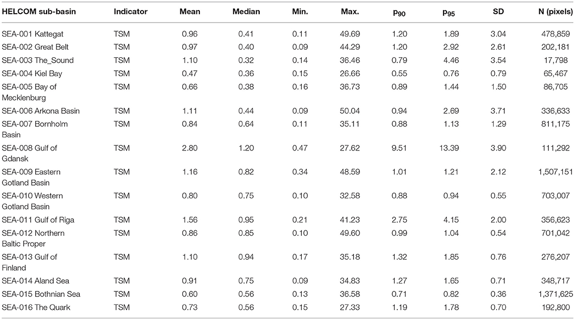
Table 3. TSM concentration per sub-basin derived from a 3-year TSM summer composite.

Results

The binned summer composites of TSM concentrations (Figure 2, upper panels) show that the distribution pattern and the coverage of filamentous cyanobacteria varies from year to year. The 3-year composite (lower panel) averaging all viable summer data (2009–2011) shows the distribution of TSM corresponding to the previous HELCOM assessment period which spanned over a five-year period (2007–2011). According to HELCOM, at least 3 consecutive years within a five-year period should be assessed in order to account for natural variability in the data. In the coastal areas, the composites indicate increased TSM due to coastal run-off, but also depict off-shore production by filamentous cyanobacteria that are usually dominant during the summer months. The summer composite from 2009 is heavily influenced by cyanobacteria blooms in the Baltic proper, with highest concentrations in Western Gotland Basin. The composite from summer 2010 showed higher TSM in the Southern Baltic (especially in the Eastern Gotland Basin), highlighting mixing processes between off-shore blooms and wind-driven resuspension of sediments. Summer 2011 was somewhat less affected by the off-shore production of filamentous cyanobacteria, apart from distinctly higher concentrations in the Northern Baltic Proper with extension towards the Gulf of Finland. The Western Baltic (along the Swedish, Danish and German coasts) showed lower TSM concentrations apart from the Pomeranian Bight. In the Bothnian Sea, there are usually no blooms of filamentous cyanobacteria detected, and the increased values of TSM on a strip along the Finnish coast observed throughout all summer seasons may indicate the influence of fluvial input and/or of other phytoplankton species. The 3-year composite in the lower panel in Figure 2 summarizes the distribution of TSM in the Baltic Sea over the 3-year period, and shows the average concentrations over the three chosen years. This 3-year summer composite was then superimposed by a shapefile, containing the last HELCOM sub-divisions of the Baltic Sea (Table 2; Figure 3). The box-and-whisker plots for the different basins (Figure 4), indicate a parabolic increase in the ranges of TSM concentration from the most Western basin up to the Baltic proper, and again decreasing values further up North, through the Bothnian Sea (SEA-015) and The Quark (SEA-016). The Gulf of Gdansk (Basin SEA-008) with its strong fluvial input and the shallow Gulf of Riga (SEA-011) showed a much wider range of TSM (0.47–27.6 gm⁻³, and 0.21–41.2 gm⁻³), and the highest Median values, 1.2 gm⁻³ and 0.95gm⁻³, respectively, than found in other basins. Furthermore, the Eastern Gotland Basin (SEA-009) showed a significantly higher median value (0.82 gm⁻³), than the Western Gotland Basin (SEA-010); (0.75 gm⁻³), the latter showing very similar median values as found in the Åland Sea. The Eastern Gotland basin (SEA-009) and the Northern Baltic Proper (SEA-012) showed a very similar range of sediment loads and median values that do not differ significantly: 0.82 gm⁻³ vs. 0.85 gm⁻³, respectively. The Gulf of Finland (SEA-013) is also characterized by somewhat higher values (median: 0.94 gm⁻³), possibly due to the very strong inflow of sediments loads from the Niva river in the Eastern Gulf of Finland (close to St. Petersburg).

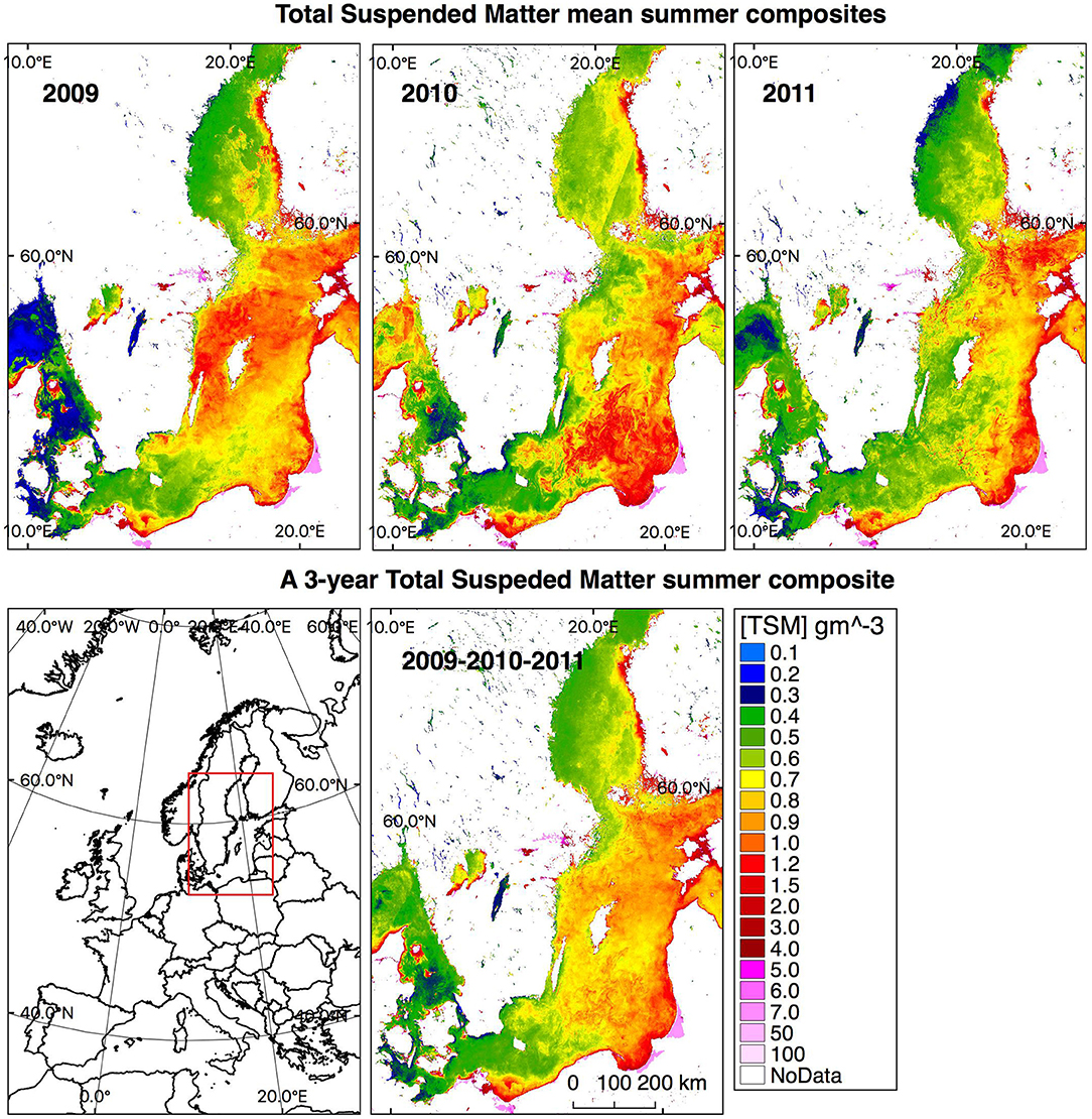
Figure 2. Total Suspended Matter mean summer concentrations (gm⁻³) in 2009, 2010, 2011, and a 3-year summer composite in the Baltic Sea. Countries (https://www.naturalearthdata.com/downloads/10m-cultural-vectors/10m-admin-0-countries/).

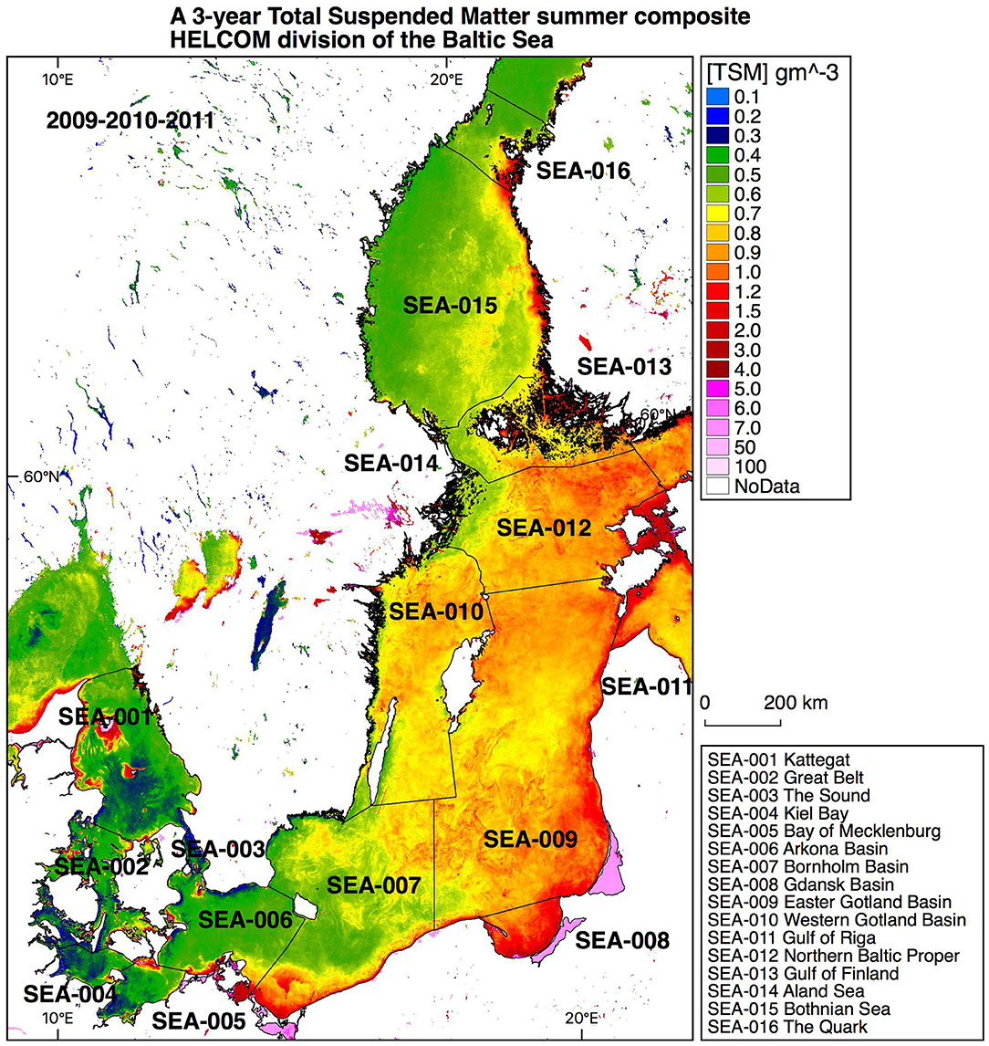
Figure 3. A 3-year TSM summer composite superimposed by HELCOM sub-basins (http://metadata.helcom.fi/geonetwork/srv/eng/catalog.search#/metadata/d4b6296c-fd19-462c-94d2-4c81b9313d77).

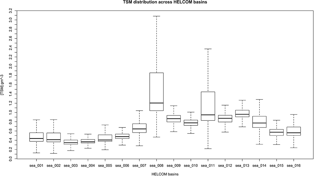
Figure 4. Box-and-whisker plot comparison of TSM concentrations (box: interquartile range; horizontal line: median; whiskers: upper and lower fence) between HELCOM basins for a 3-year summer composite.

In order to evaluate the differences in coastal distribution patterns, a transect was extracted through Himmerfjärden bay from each composite (2009–2011), and also from the 3-year seasonal composite (2009–2011). Each transect represents a gradient from the inner-most part of Himmerfjärden bay, toward the open sea. The values extracted along the coastal-open sea transect are shown in Figure 5. The extracted TSM concentrations were plotted against the distance to the Himmerfjärden Sewage Treatment Plant (STP) situated in the inner bay (Figure 1, right panel). The descriptive statistical parameters i.e., the mean, median, minimum, maximum, the standard deviation (SD) and the number of pixels (N), respectively, for each season along the transect were derived and summarized in Table 4. The TSM values extracted along the transect indicate that the mean concentrations in the summer seasons 2009 and 2011 were almost the same, whereas the median was higher (1.07 gm⁻³) during 2011. The summer season 2010 was described by lower TSM concentrations and variability along the transect. There was a clear decline of TSM concentrations at a distance of about 30 km from the sewage treatment plant. This corresponds to the mouth of Himmerfjärden, that is delineated by a sill and by Askö island (Figure 1, right panel). The concentrations further off-shore decrease asymptotically. Summer 2011 was strongly influenced by open sea production (i.e., a cyanobacteria bloom) that is clearly visible on the map (Figure 2 top right panel; Figure 4), and represented on the corresponding plot by high variability in concentrations both before and after the 30 km mark. The transect extracted from the 3-year composite shows the mean coastal gradient of TSM distribution along the coast with a median concentration of 0.9 gm⁻³ and a mean of 1.0 gm⁻³, which is within ranges of the median (1.5 gm⁻³; 2008–2014) and mean (1.4 gm⁻³; 2001–2002) measured in situ in this area (Kratzer and Tett, 2009; Kari et al., 2017), although the values derived from MERIS are underestimated by approximately 1/3.

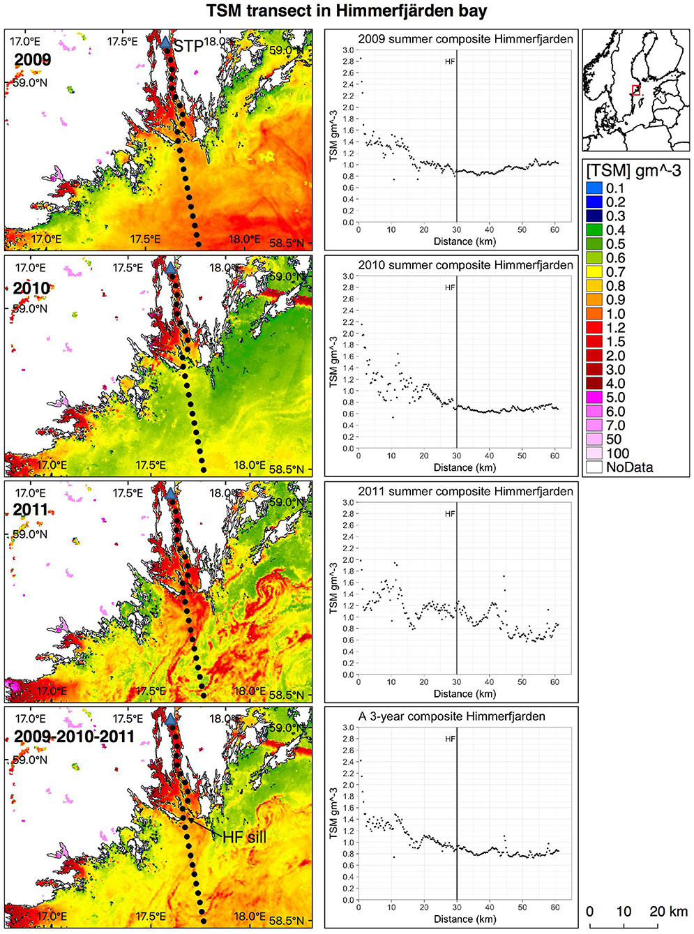
Figure 5. TSM transect derived from composites of three summer seasons 2009, 2010, 2011, and a 3-year summer composite, Himmerfjaärden bay, Sweden. European coastline shapefile (see caption Figure 1). Transect plots (R-studio 3.4.1; {ggplot2} package; Wickham, 2016).

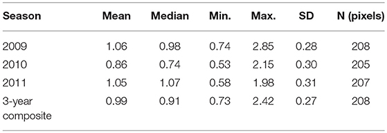
Table 4. Comparison of TSM concentration per transect derived from summer seasons 2009–2011 and a 3-year summer composite.

In the following we compare the TSM concentrations derived from the 3-year summer composite and extracted for the different HELCOM sub-basin to in situ measured values found in the literature. Arkona Basin (SEA-004): 0.1–50.4 gm⁻³ derived from satellite vs. 0.7–9.0 gm⁻³ (Ohde et al., 2007; Fleming-Lehtinen and Laamanen, 2012). Bornholm Basin (SEA-007): 0.1–35.1 gm⁻³ vs. 0.4–5.0 gm⁻³ (Ohde et al., 2007; Fleming-Lehtinen and Laamanen, 2012) and 0.5–20.0gm⁻³ (Ohde et al., 2007; Fleming-Lehtinen and Laamanen, 2012). Eastern Gotland Basin (SEA-009): 0.3–48.5 gm⁻³ vs. 3.0–6.0 gm⁻³ (Ohde et al., 2007; Fleming-Lehtinen and Laamanen, 2012); and 1.1–32.0 gm⁻³ (Wasmund et al., 2001; Vaičiute et al., 2012). Gulf of Gdansk (SEA-008): 0.5–27.6 gm⁻³ vs. 0.4–15.7 gm⁻³ (Ohde et al., 2007; Fleming-Lehtinen and Laamanen, 2012). Gulf of Riga (SEA-011): 0.2–41.2 gm⁻³ vs. 10.0 - 24.0 gm⁻³ (Toming et al., 2009; Fleming-Lehtinen and Laamanen, 2012; Raag et al., 2014). Gulf of Finland (SEA-013): 0.2–35.1 gm⁻³ vs. 0.8–20.0 gm⁻³ (Toming et al., 2009; Fleming-Lehtinen and Laamanen, 2012; Raag et al., 2014). Western Gotland Basin (SEA-010): 0.1–32.5 gm⁻³ vs. 0.5–21.7 gm⁻³ (Toming et al., 2009; Fleming-Lehtinen and Laamanen, 2012; Raag et al., 2014). Bothnian Sea (SEA-015) 0.1–36.5 gm⁻³ vs. 0.2–20.9 gm⁻³ (Toming et al., 2009; Fleming-Lehtinen and Laamanen, 2012; Raag et al., 2014). Overall, it may be stated that the ranges of TSM measured in situ are also covered by the 3-year composite MERIS data. However, for each basin the satellite data shows a much higher range.

Discussion

Recent advances in ocean color remote sensing led to the development of reliable coastal processors such as the coastal water properties processor developed by Free University of Berlin (FUB). This processor allows for the reliable retrieval of in-water constituents from satellite data also over optically-complex waters with high CDOM absorption. The use of the FUB processor here to derived TSM combined with data quality flags developed in the CoastColor project (C2R CoastColor) allowed to derive a 3-year summer composite, covering almost the whole Baltic Sea. The frequent cloud cover (40–55%) during the summer period in the Baltic Sea (Karlsson, 2003), makes it a challenge to get cloudless images and to evaluate the spatial distribution of in-water constitutes e.g., TSM on a daily-basis. In order to get full spatial coverage of the entire basin it is required to aggregate several daily images together into weekly, monthly or seasonal averages. Often, there are not enough complete daily scenes to produce representative monthly averages. Those scenes, however, can be accounted for in the seasonally-averaged summer composite presented in this study. There are statistical methods (Poggio et al., 2012; Weiss et al., 2014; Land et al., 2018), to fill in the gaps caused by flagged pixels (e.g., cloud flags), but these methods may also be prone to error.

The TSM images derived from MERIS data and presented here showed to be relevant for mapping areas with high run-off and also highlight regional differences in coastal influence, such as in the Western Baltic Sea (Figure 3). TSM also indicates large-scale oceanographic features, such as eddies influencing the TSM distribution in the Southern and Eastern Baltic Sea, and carrying the sediments off-shore, and also further up North along the Eastern Baltic coast. The typical long-term mean horizontal current field in the Baltic Sea has a weak cyclonic pattern, creating anti-clockwise, rotation across the Baltic proper (Kullenberg, 1981; Stigebrandt, 2001). This rotation leads to the so-called Swedish current that transports surface waters up North (on the Eastern side of the Basin), and down south all along the Swedish coast (Voipio, 1981). TSM is also indicative of meso-scale features generated by atmospheric Rossby, i.e., planetary atmospheric waves caused by the Coriolis acceleration as well as by bottom topography and friction (Lehmann and Myrberg, 2008). Another common phenomenon is coastal upwelling, usually observed in the summer season along the Baltic Sea coastline at distances of approximately 10–20 km off-shore (Lehmann and Myrberg, 2008). The overlap between coastal sediment plumes and currents carrying suspended matter both further off-shore, and further up North along the Finnish coast is visible on the TSM composites (Figures 2, 3). Strong wind-wave stirring in the Southern Baltic keeps small and medium sized particles (Danielsson et al., 2007) as well as organic suspended matter longer in suspension, and moves them further off-shore.

Besides depicting large-scale phenomena, seasonal averages also allow for a comparison between summer seasons from different years, and also aggregation into longer time-periods, such as the 3-year summer composite presented in this study. These images may be used in management as complimentary information for the status classification of the Baltic Sea e.g., in the periodic assessments done by HELCOM.

Comparison of Different Baltic Sea Basins

The superimposing of the HELCOM division of the Baltic Sea into 16 sub-basins allowed to evaluate the 3-year summer composite of TSM with respect to HELCOM basins. Concentrations in the different basins were then compared statistically. Figure 4 illustrates that the ranges of TSM concentrations vary between basins, indicating the presence of cyanobacteria blooms as well as influence from physical processes such as wind-wave stirring and resuspension of sediments in shallow areas (Jönsson, 2005; Danielsson et al., 2007). Danielsson et al. (2007) found that these events have seasonal patterns with higher resuspension frequency in winter due to stronger current velocities. They also found that grain size had a strong effect, with fine sediments and medium sand having a considerable higher percentage of resuspension than larger grain sizes. As cyanobacteria and other phytoplankton are mostly made up of organic matter, and sometimes even may have positive buoyancy–e.g., due to the gas vacuoles in filamentous cyanobacteria (Walsby et al., 1995), they can be carried much further off-shore, following the dominant oceanographic currents.

The Gulf of Gdansk (sea_009) and Gulf of Riga (sea_011) include wider ranges of TSM, compared to the other basins. Both are coastal basins that are relatively shallow (the Gulf of Gdansk has a mean depth of 57 m and the Gulf of Riga 23 m) and may be exposed to strong wind-wave stirring, keeping the suspended matter in suspension (Danielsson et al., 2007). These processes, in turn, are manifested in higher concentrations of TSM, and the mean values are depicted in the satellite images (Figure 2), and are statistically compared in Table 3. The Gulf of Gdansk also receives considerable amounts of terrestrial input from the Vistula river (Szymczak and Galinska, 2013). The Gulf of Riga was only partially captured by the analyzed composite and the results may thus not capture the full variability of TSM in this basin. This highlights the challenges collecting remote sensing data in the Baltic Sea region—which has a relatively high occurrence of cloud cover (Karlsson, 2003).

In the Northwestern Baltic proper TSM concentrations are generally much lower and reach much less further off-shore than in the Southern and Southeastern Baltic proper. Also, the sea bottom here predominantly consists of exposed rock and mud, whereas the bottom substrate in S and SE Baltic proper is dominant by sand and mud (Al-Hamdani and Reker, 2007). In the Southern Baltic Sea, the TSM concentrations are presumably higher due to the higher run-off from large rivers in the Southern Baltic (i.e., the Vistula and the Order) and due to stronger wind exposure (Danielsson et al., 2007). Here, wind-wave stirring may keep the heavier particles in suspension longer and carry it further off-shore by the surface currents. The southern Baltic Sea is also characterized by a different morphology, hydrology and bottom topography. The coast is rather exposed to wind and there are only a limited number of large bays (such as the Gulf of Riga and the Gulf of Gdansk). The NW Baltic has a completely different morphology with a large number of elongated bays that often consist of small sub-basins intersected by sills, and it is less exposed to wind (Danielsson et al., 2007). Heavy inorganic particles thus tend to fall out here in the inner basins.

It is also the combination of bottom topography and river run-off that seem to determine the TSM loads in the more coastal basins in the Southern and in the Eastern Baltic. Large rivers (i.e., the Oder and Vistula in the South as well as the Neva in the East) bring in large amounts of anthropogenic loads from densely populated areas in Poland, Germany and Russia. Figures 3, 4 show that the Gulf of Gdansk (SEA-008), the Eastern Gotland Basin (SEA-009), and the Gulf of Riga (SEA-11) stick out with clearly elevated values of TSM. For the Gulf of Gdansk and the Gulf of Riga, this may be attributed to strong coastal influence and shallow bottom topography—especially in the Gulf of Riga- as well as cyanobacterial production during summer. In the off-shore areas of the Eastern Gotland Basin (SEA-009) cyanobacterial production seems to dominate the picture. The Northern Baltic proper (SEA-12) the Eastern Gotland Basin (SEA-009) and the Western Gotland Basin (SEA-010) showed similar patterns of off-shore TSM that seem to be strongly influenced by cyanobacteria blooms. The Arkona Basin (SEA-006) and the Bothnian Sea (SEA-015) seem least influenced by wind-driven resuspension and/or blooms of filamentous cyanobacteria. Filamentous cyanobacteria generally do not tend to bloom in the Gulf of Bothnia, which may be partially attributed to phosphate limitation (Snoeijs-Leijonmalm et al., 2017). Also, the lower water temperatures (subarctic, boreal climate) and the low salinities (ranging from 1.8 g kg⁻¹ up North in the Bothnian Bay to 6.6 g kg⁻¹ in the Bothnian Sea), as well as the low water transparencies (Snoeijs-Leijonmalm et al., 2017) may limit cyanobacterial growth (Lehtimaki et al., 1997). The accumulation patterns of particulate matter are strongly related both to sediment type and basin depth (Leipe et al., 2011). The Arkona Basin (SEA-006) basin, however, is relatively shallow with a mean depth of 23 m. Despite the shallowness, Leipe et al. (2011) found relatively low accumulation rates of particulate organic matter in the Arkona Sea. The authors state that large differences in the accumulation and burial rates of organic matter cannot always be fully explained by regional differences in surface-water productivity. The deep water transport in the Baltic Sea happens in a cascade-like manner from the shallower into the deeper basins (Voipio, 1981) and suspended sediments thus tend to accumulate in the deepest basins such as the Gotland basin (Leipe et al., 2011).

Trend in Himmerfjärden Bay

The inner coastal to off-shore transects extracted from the TSM composites from the 3 different summer seasons in Himmerfjärden showed that TSM follows a rather steep decrease inside Himmerfjärden bay, tending toward an asymptotic line in the open sea. This trend was first observed and described by Kratzer and Tett (2009), using in situ data from summer, and is now confirmed here by transects derived from MERIS data, indicating a similar distribution trend. Kratzer and Tett (2009) showed that the high concentrations of TSM in the inner bay are mostly caused by inorganic particles which fall out rather steeply in the inner bay. The TSM found in the open sea consisted mostly of organic particles (including phytoplankton), which tend to be lighter, and thus can be carried further off-shore. These trends were recently confirmed in a spring study by Kari et al. (2018), which also confirmed a much higher percentage of inorganic material in the inner bay during spring time. These patterns again seem to be governed by a combination of bottom topography (small sub-basins intersected by sills) and the relatively low wind forcing in the NW Baltic Sea.

The in situ TSM transect described by Kratzer and Tett (2009) was derived from the mean of 4 optical transects measured during June 2001 and August 2002, and thus originated both from different years and from different summer months. Compared to the TSM transects derived from MERIS data, the in situ transects were spatially sparse (3–5 optical station in each transect with about 15–20 km distance between stations). In contrast, the transects derived from MERIS TSM composites were derived from full spatial resolution data (300 m pixels), allowing to derive a continuous set of TSM concentrations, and to fill in the gaps between the in situ sampling stations. The results shown in Figure 5 demonstrate that there is a consistent trend with higher values in the inner bay that is also persistent through different summer seasons. The study by Kari et al. (2018) confirmed that the same spatial pattern is also found in spring with slightly higher ranges of TSM due to the influence from ice thawing. The higher range of values in coastal waters can be attributed to the influence from land (erosion and run-off). The strong variability of TSM in the open sea during summer can be mostly explained by the variability in cyanobacteria biomass (Kratzer and Tett, 2009; Beltrán-Abaunza et al., 2016; Kari et al., 2017).

The remote sensing approach also allows to retrieve and assess the variability and distribution of TSM concentrations between stations. As in situ measurements are relatively expensive and much more time consuming, one usually samples at a much lower spatial, and temporal resolution than possible to retrieve from satellite data (Beltrán-Abaunza et al., 2016; Harvey et al., 2018). Additionally, similar transects derived in other regions of the Baltic Sea allow to spatially evaluate the contribution of river run-off and coastal resuspension (Kyryliuk, 2014). For example, rivers that flow through agricultural landscapes transport suspended sediments and nutrients. Agricultural run-off rich in nutrients as well as industrial discharges are prime contributors of phosphorus and nitrogen into surface waters that may also affect off-shore eutrophication (Voipio, 1981). Suspended matter often contains phosphorus and is transported from coastal areas into the open Baltic Sea, following currents. The sediment transport is also influenced by wind-stirring as wind may cause resuspension of sediments that, in turn, may affect the nutrient dynamics (Danielsson et al., 2007). All these processes are reflected in the TSM patterns that are visible from space and can be quantified and mapped. As TSM and total phosphate are correlated (Beusekom and Jonge, 1994), one possibly could also use satellite-derived TSM as a proxy for phosphorus distribution in coastal areas or in different basins of the Baltic Sea.

Furthermore, TSM is highly related to turbidity as TSM scatters light and turbidity is a measure of particle scatter. This relationship has been studied by Kari et al. (2017) and has shown to be robust across the Baltic Sea. The authors developed a regional algorithm between TSM and turbidity in the Baltic Proper and tested the algorithm on independent datasets, including a dataset from Lithuanian coastal waters and the Curonian Lagoon with very large ranges of TSM (0.6–24.0 gm⁻³ and 1.8–34.0 gm⁻³, respectively). The r² for the TSM-turbidity relationship was found to be 0.93 (Kari et al., 2017; Kari, 2018). According to the nomenclature of the EU Water Framework Directive TSM could also be described as a physio-chemical parameter. Turbidity is listed in the EU Marine Strategy Framework directive as one of the mandatory variables to be measured and monitored in coastal waters (Marine Strategy Framework Directive Annex III, 2008). The concentrations of TSM—and thus turbidity—can also be used as an indicator for coastal water masses (Capello et al., 2004; Kratzer and Tett, 2009; Almroth-Rosell et al., 2011).

A number of studies have been conducted in recent years (Table 1) where researchers measured TSM in situ in different Baltic Sea basins. Although monitoring campaigns and oceanographic cruises are quite regular in the Baltic Sea, they still cannot achieve the same temporal and spatial coverage as satellite data. In situ campaigns usually cover open sea station as well as coastal areas. They most often take place in spring in order to track the development of the spring bloom (that consists mostly of diatoms and dinoflagellates), and then later in summer to cover the cyanobacteria blooms. However, sampling campaigns are logistically rather complex and are associated with high costs and usually limited to a set of pre-defined stations that are revisited yearly to keep track of the annual variability of water quality variables. These spatially sparse monitoring stations are often considered to be representative for each basin. However, in reality they are only very limited point measurements and even sometimes only represent one point in time in the respective basin. The Baltic Sea, however, is highly variable and dynamic, as shown in Figure 2, and what happens between stations or where measurements are not performed at all is often assumed or calculated by means of numerical modeling (Savchuk, 2018), which, again, is often based on a restricted number (both in space and in time) of empirical/measured data.

Ocean color data provides us with waters quality indicators (e.g., CDOM, chl-a, TSM and Secchi depth) that are also routinely measured in situ (Kratzer et al., 2016). Extensive validation campaigns and development of improved algorithms to derive the inherent optical properties and in-water constituents from remote sensing reflectance data allows to derive water quality indicators reliably and with full spatial resolution (300 m) on a Baltic Sea wide scale (Kutser et al., 2005; Ohde et al., 2007; Kratzer et al., 2008, 2011; Kutser, 2009; Kratzer and Vinterhav, 2010; Vaičiute et al., 2012; Beltrán-Abaunza et al., 2014; Kahru and Elmgren, 2014; Hieronymi et al., 2017; Kari et al., 2017; Kratzer and Moore, 2018). This body of recent research demonstrates that the remote sensing approach corresponds to the MSP needs for high quality data and assessment tools with high temporal and spatial resolution.

Furthermore, GIS analysis of MERIS-derived TSM data allows to retrieve concentrations for any bay, estuary or basin larger than 300 m. The HELCOM sub-divisions of the Baltic Sea comes with a shapefile that can be used to derive basin-specific concentrations, to statistically estimate the difference between those basins, and also to evaluate how those concentrations compare to what is found in the literature. The comparison here showed that concentrations derived from the TSM composite indicate much wider ranges than measured in situ and found in the literature (see Tables 1, 3), possibly due to a better spatial coverage by satellite data. However, the very high ranges may also be due to inclusion of very near-shore areas (pixels), where TSM retrieval may be influenced by the so-called land-adjacency effect, i.e., the high reflectance from land that may influence near-shore water pixels. This, in turn may lead to erroneously high values of TSM concentrations (Toming et al., 2017). Statistically, this can be accounted for by either using the median values (accounting for non-normal distribution of the data), or by using the 90 or 95 percentiles excluding the extreme values, and thus accounting for errors associated with land-adjacency effects and values that are beyond the training range of a given processor.

Conclusion

The use of the FUB processor on MERIS data over the Baltic Sea allowed to map the summer distribution of TSM over the last 3 years of the ENVISAT mission. This time span also fell within HELCOM's previous assessment period (2007–2011). The problems related to frequent cloud cover in the Baltic Sea, leading to limited coverage of individual MERIS scenes, could be overcome by producing averaged summer composite using the L3 binning approach. This allowed to map the TSM distribution almost across the entire Baltic Sea basin (apart from some areas in the Gulf of Riga and the Gulf of Finland due extensive cloud cover). The summer composites from 2009 to 2011 were aggregated into a single 3-year summer season composite, representing average spatial patterns of TSM distribution over this time period. These composites demonstrate how ocean color remote sensing data can provide additional information for Baltic Sea research and management. It allows to understand and investigate large-scale phenomena, from river discharge and phytoplankton blooms, to meso-scale features, depicting the mean current-fields of the Baltic Sea, to the monitoring of coastal waters. The main advantage to conventional monitoring efforts is a synoptic and potentially full-scale coverage of the Baltic Sea with good spatial and temporal resolution (Kratzer et al., 2014; Harvey et al., 2018). The additional use of GIS allowed to divide the 3-year summer composite into sub-basins according to HELCOM designated basins, and to derive descriptive statistics for each corresponding basin, and to perform a spatial trend analysis on an extracted coastal transects from Himmerfjärden bay and adjacent areas. TSM particles followed a steep decline in the inner-most part of the bay and converted toward relatively low open sea values ranging from about 0.5–0.7 gm⁻³. The trend showed to fluctuate, depending on the conditions during the respective summer season, e.g., due to variability in precipitation, run-off and coastal primary production as well as the influence of off-shore production- e.g., cyanobacterial blooms- further off the coast. The transects confirmed observations and trends previously made using in situ measurements, namely a rather steep decline of TSM in inner coastal bay, tending toward an open sea threshold. Such data extracted from coastal transects may play a role in estimating water exchange rates within coastal and open sea systems, and the ecological state of these systems. Furthermore, this approach allowed to fill in gaps between monitoring stations, describing coastal trends with good spatial resolution and coverage. TSM concentration extracted from a 3-year summer composite showed to be coherent with values found in the literature, however with somewhat larger ranges.

Author Contributions

All authors listed have made a substantial, direct and intellectual contribution to the work, and approved it for publication.

Funding

This research was funded by Swedish National Space Board (SNSB) contract no. Dnr. 165/11 and Dnr. 175/17, European Space Agency (ESA)/ESRIN contract no. 21524 and by SU's strategic project Baltic Ecosystem Adaptive Management (BEAM), application no. 2009-3435-13495-18.

Conflict of Interest Statement

The authors declare that the research was conducted in the absence of any commercial or financial relationships that could be construed as a potential conflict of interest.

Acknowledgments

The satellite imagery and detailed information on data processing was provided by Dr. Petra Phillipson, Brockmann Geomatics, Sweden AB. Thanks to Brockmann Consult, Germany for data processing up to Level-2 (Pre-processing and FUB). Thanks to Kari Eilola for helpful comments on a previous version of the manuscript.

References

Al-Hamdani, Z., and Reker, J. (eds.). (2007). Towards marine landscapes in the Baltic Sea. Balance interim report #10. Copenhagen. Available online at: http://balance-eu.org/xpdf/balance-interim-report-no-10.pdf (Accessed December 20, 2018).
Alikas, K., Kratzer, S., Reinart, A., Kauer, T., and Paavel, B. (2015). Robust remote sensing algorithms to derive the diffuse attenuation coefficient for lakes and coastal waters. Limnol. Oceanogr. Methods 13, 402–415. doi: 10.1002/lom3.10033
Almroth-Rosell, E., Eilola, K., Hordoir, R., Meier, M. H. E., and Hall, P. (2011). Transport of fresh and resuspended particulate organic material in the Baltic Sea — a model study. J. Mar. Syst. 87, 1–12. doi: 10.1016/j.jmarsys.2011.02.005
Beltrán-Abaunza, J. M., Kratzer, S., and Brockmann, C. (2014). Evaluation of MERIS products from Baltic Sea coastal waters rich in CDOM. Ocean Sci. 10, 377–396. doi: 10.5194/os-10-377-2014
Beltrán-Abaunza, J. M., Kratzer, S., and Höglander, H. (2016). Using MERIS data to assess the spatial and temporal variability of phytoplankton in coastal areas. Int. J. Remote Sens. 38, 2004–2028. doi: 10.1080/01431161.2016.1249307
Beusekom, J. E. E., and Jonge, V. N. (1994). The role of suspended matter in the distribution of dissolved inorganic phosphate, iron and aluminium in the Ems estuary. Netherlands J. Aquat. Ecol. 28, 383–395. doi: 10.1007/BF02334208
Bourg, L., D'Alba, L., and Colagrande, P. (2008). MERIS Smile Effect Characterization and Correction. Paris: ESA. Available online at: https://earth.esa.int/documents/700255/707220/MERIS_Smile_Effect.pdf/a1e7cbd0-2f1e-40f2-a5bc-92f5dab1ee43 (Accessed December 20, 2018).
Capello, M., Budillon, G., Ferrari, M., and Tucci, S. (2004). Suspended matter variability in relation to water masses in Terra Nova Bay (Ross Sea-Antarctica). Chem. Ecol. 20, S7–S18. doi: 10.1080/02757540410001664620
Danielsson, Å., Jönsson, A., and Rahm, L. (2007). Resuspension patterns in the Baltic proper. J. Sea Res. 57, 257–269. doi: 10.1016/j.seares.2006.07.005
Devlin, M. J., Barry, J., Mills, D. K., Gowen, R. J., Foden, J., Sivyer, D., et al. (2008). Relationships between suspended particulate material, light attenuation and Secchi depth in UK marine waters. Estuar. Coast. Shelf Sci. 79, 429–439. doi: 10.1016/j.ecss.2008.04.024
Dogliotti, A. I., Ruddick, K. G., Nechad, B., Doxaran, D., and Knaeps, E. (2015). A single algorithm to retrieve turbidity from remotely-sensed data in all coastal and estuarine waters. Remote Sens. Environ. 156, 157–168. doi: 10.1016/j.rse.2014.09.020
Engqvist, A. (1996). Long-term nutrient balances in the eutrophication of the Himmerfjärden estuary. Estuar. Coast. Shelf Sci. 42, 483–507. doi: 10.1006/ecss.1996.0031
Fleming-Lehtinen, V., and Laamanen, M. (2012). Long-term changes in Secchi depth and the role of phytoplankton in explaining light attenuation in the Baltic Sea. Estuar. Coast. Shelf Sci. 102–103, 1–10. doi: 10.1016/j.ecss.2012.02.015
Franzén, F., Kinell, G., Walve, J., Elmgren, R., and Söderqvist, T. (2011). Participatory social-ecological modeling in eutrophication management: the case of Himmerfjärden, Sweden. Ecol. Soc. 16:art27. doi: 10.5751/ES-04394-160427
Harvey, E. T., Walve, J., Andersson, A., Karlson, B., and Kratzer, S. (2018). The effect of optical properties on secchi depth and implications for eutrophication management. Front. Mar. Sci. 5:496. doi: 10.3389/fmars.2018.00496
Harvey, T. (2015). Bio-optics, Satellite Remote Sensing and Baltic Sea Ecosystems: Applications for Monitoring and Management. Doctoral dissertation, Department of Ecology, Environment and Plant Sciences, Stockholm University. Available online at: http://www.diva-portal.org/smash/record.jsf?pid=diva2%3A849120&dswid=3680 (Accessed December 20, 2018).
Hieronymi, M., Müller, D., and Doerffer, R. (2017). The OLCI Neural Network Swarm (ONNS): a bio-geo-optical algorithm for open ocean and coastal waters. Front. Mar. Sci. 4:140. doi: 10.3389/fmars.2017.00140
Hijmans, R. J., van Etter, J., Cheng, J., Mattiuzzi, M., Summer, M., Greenberg, J. A., et al. (2017). Geographic Data Analysis and Modeling. R CRAN Proj. Available online at: http://rspatial.org/ (Accessed December 20, 2018).
Jönsson, A. (2005). Model Studies of Surface Waves and Sediment Resuspension in the Baltic Sea. Available online at: http://www.diva-portal.org/smash/get/diva2:20699/FULLTEXT01.pdf.
Kahru, M., and Elmgren, R. (2014). Multidecadal time series of satellite-detected accumulations of cyanobacteria in the Baltic Sea. Biogeosciences 11, 3619–3633. doi: 10.5194/bg-11-3619-2014
Kahru, M., Savchuk, O. P., and Elmgren, R. (2007). Satellite measurements of cyanobacterial bloom frequency in the Baltic Sea: interannual and spatial variability. Mar. Ecol. Prog. Ser. 343, 15–23. doi: 10.3354/meps06943
Kari, E. (2018). Light Conditions in Seasonally Ice-Covered Waters : Within the Baltic Sea Region. Available online at: http://su.diva-portal.org/smash/get/diva2:1221600/FULLTEXT01.pdf
Kari, E., Kratzer, S., Beltrán-Abaunza, J. M., Harvey, E. T., and Vaičiute, D. (2017). Retrieval of suspended particulate matter from turbidity – model development, validation, and application to MERIS data over the Baltic Sea. Int. J. Remote Sens. 38, 1983–2003. doi: 10.1080/01431161.2016.1230289
Kari, E., Merkouriadi, I., Leppäranta, M., Walve, J., and Kratzer, S. (2018). Development of under-ice stratification in Himmerfjärden bay, north-western Baltic proper, and their effect on the phytoplankton spring bloom. Mar J. Syt. 186, 85–95. doi: 10.1016/j.jmarsys.2018.06.004
Karlsson, K.-G. (2003). A 10 year cloud climatology over Scandinavia derived from NOAA advanced very high resolution radiometer imagery. Int. J. Climatol. 23, 1023–1044. doi: 10.1002/joc.916
Kirk, J. T. O. (1985). Light and photosynthesis in aquatic ecosystems. Int. Rev. der gesamten Hydrobiol. und Hydrogr. 70, 897–898. doi: 10.1002/iroh.19850700619
Kopelevich, O. V., Vazyulya, S. V., Sheberstov, S. V., and Bukanova, T. V. (2016). Suspended matter in the surface layer of the southeastern Baltic from satellite data. Oceanology 56, 46–54. doi: 10.1134/S0001437016010069
Koponen, S., Attila, J., Pulliainen, J., Kallio, K., Pyhälahti, T., Lindfors, A., et al. (2007). A case study of airborne and satellite remote sensing of a spring bloom event in the Gulf of Finland. Cont. Shelf Res. 27, 228–244. doi: 10.1016/j.csr.2006.10.006
Kowalczuk, P., Olszewski, J., Darecki, M., and Kaczmarek, S. (2005). Empirical relationships between coloured dissolved organic matter (CDOM) absorption and apparent optical properties in Baltic Sea waters. Int. J. Remote Sens. 26, 345–370. doi: 10.1080/01431160410001720270
Kowalczuk, P., Stedmon, C. A., and Markager, S. (2006). Modeling absorption by CDOM in the Baltic Sea from season, salinity and chlorophyll. Mar. Chem. 101, 1–11. doi: 10.1016/j.marchem.2005.12.005
Kratzer, S. (2000). Bio-Optical Studies of Coastal Waters. Ph.D. Thesis, School of Ocean Sciences, University of Wales, Bangor, UK. Available online at: http://www.isni.org/isni/0000000136024205
Kratzer, S., Alikas, K., Harvey, T., Beltrán-Abaunza, J. M., Morozov, E., Mustapha, S. B., et al. (2016). “Multitemporal remote sensing of coastal waters,” in Multitemporal Remote Sensing: Methods and Applications, ed. Y. Ban (Cham: Springer International Publishing), 391–426. doi: 10.1007/978-3-319-47037-5_19
Kratzer, S., Brockmann, C., and Moore, G. (2008). Using MERIS full resolution data to monitor coastal waters - A case study from Himmerfjarden, a fjord-like bay in the northwestern Baltic Sea. Remote Sens. Environ. 112, 2284–2300. doi: 10.1016/j.rse.2007.10.006
Kratzer, S., Ebert, K., and Sørensen, K. (2011). “Monitoring the bio-optical state of the Baltic Sea ecosystem with remote sensing and autonomous in situ techniques,” in The Baltic Sea Basin, eds. J. Harff, S. Björck, and P. Hoth (Berlin; Heidelberg: Springer), 407–435. doi: 10.1007/978-3-642-17220-5_20
Kratzer, S., Håkansson, B., and Sahlin, C. (2003). Assessing Secchi and photic zone depth in the Baltic Sea from satellite data. J. Hum. Environ. 32, 577–585. doi: 10.1639/0044-7447(2003)032[0577:asapzd]2.0.co;2
Kratzer, S., and Moore, G. (2018). Inherent optical properties of the baltic sea in comparison to other seas and oceans. Remote Sens. 10:418. doi: 10.3390/rs10030418
Kratzer, S., and Tett, P. (2009). Using bio-optics to investigate the extent of coastal waters: a Swedish case study. Hydrobiologia 629, 169–186. doi: 10.1007/s10750-009-9769-x
Kratzer, S., Therese Harvey, E., and Philipson, P. (2014). The use of ocean color remote sensing in integrated coastal zone management—A case study from Himmerfjärden, Sweden. Mar. Policy 43, 29–39. doi: 10.1016/j.marpol.2013.03.023
Kratzer, S., and Vinterhav, C. (2010). Improvement of MERIS level 2 products in baltic sea coastal areas by applying the improved Contrast between Ocean and Land Processor (ICOL) - Data analysis and validation. Oceanologia 52, 211–236. doi: 10.5697/oc.52-2.211
Kuhrts, C., Fennel, W., and Seifert, T. (2004). Model studies of transport of sedimentary material in the western Baltic. J. Mar. Syst. 52, 167–190. doi: 10.1016/j.jmarsys.2004.03.005
Kullenberg, G. (1981). Chapter 3 Physical Oceanography. Elsevier Oceanogr. Ser. 30, 135–181. doi: 10.1016/S0422-9894(08)70140-5
Kullenberg, G., and Jacobsen, T. S. (1981). The Baltic Sea: an outline of its physical oceanography. Mar. Pollut. Bull. 12, 183–186. doi: 10.1016/0025-326X(81)90168-5
Kutser, T. (2009). Passive optical remote sensing of cyanobacteria and other intense phytoplankton blooms in coastal and inland waters. Int. J. Remote Sens. 30, 4401–4425. doi: 10.1080/01431160802562305
Kutser, T., Pierson, D. C., Kallio, K. Y., Reinart, A., and Sobek, S. (2005). Mapping lake CDOM by satellite remote sensing. Remote Sens. Environ. 94, 535–540. doi: 10.1016/j.rse.2004.11.009
Kyryliuk, D. (2014). Total suspended matter derived from MERIS data as an indicator of coastal processes in the Baltic Sea. Independen. Available online at: http://su.diva-portal.org/smash/get/diva2:1060672/FULLTEXT01.pdf
Land, P. E., Shutler, J. D., and Smyth, T. J. (2018). Correction of sensor saturation effects in MODIS oceanic particulate inorganic carbon. IEEE Trans. Geosci. Remote Sens. 56, 1466–1474. doi: 10.1109/TGRS.2017.2763456
Lehmann, A., and Myrberg, K. (2008). Upwelling in the Baltic Sea - A review. J. Mar. Syst. 74, 3–12. doi: 10.1016/j.jmarsys.2008.02.010
Lehtimaki, J., Moisander, P., Sivonen, K., and Kononen, K. (1997). Growth, nitrogen fixation, and nodularin production by two baltic sea cyanobacteria. Appl. Environ. Microbiol. 63, 1647–1656.
Leipe, T., Tauber, F., Vallius, H., Virtasalo, J., Uścinowicz, S., Kowalski, N., et al. (2011). Particulate organic carbon (POC) in surface sediments of the Baltic Sea. Geo Mar. Lett. 31, 175–188. doi: 10.1007/s00367-010-0223-x
Leppäranta, M., and Myrberg, K. (2009). Physical Oceanography of the Baltic Sea. Berlin; Heidelberg: Springer Berlin Heidelberg. doi: 10.1007/978-3-540-79703-6
Manual, S. U., and Document, I. C. (2007). The AMORGOS MERIS CFI (Accurate MERIS Ortho-Rectified Geo-location Operational Software) Software User Manual & Interface Control Document. Manual, Software User Document Control.
Marine Strategy Framework Directive Annex III (2008). Directive 2008/56/EC of the European Parliament and of the Council. Off. J. Eur. Union 164, 19–40. Available online at: https://eur-lex.europa.eu/legal-content/EN/TXT/PDF/?uri=CELEX:32008L0056&from=EN (Accessed December 20, 2018).
Morel, A., and Prieur, L. (1977). Analysis of variations in ocean color. Limnol. Oceanogr. 22, 709–722. doi: 10.4319/lo.1977.22.4.0709
Myrberg, K., and Lehmann, A. (2013). “Topography, hydrography, circulation and modelling of the Baltic Sea,” in Preventive Methods for Coastal Protection, eds T. Soomere, and E. Quak (Heidelberg: Springer International Publishing), 31–64. doi: 10.1007/978-3-319-00440-2_2
Ohde, T., Siegel, H., and Gerth, M. (2007). Validation of MERIS Level-2 products in the Baltic Sea, the Namibian coastal area and the Atlantic Ocean. Int. J. Remote Sens. 28, 609–624. doi: 10.1080/01431160600972961
Patrice, B., Amberg, V., Bourg, L., PETIT, D., Huc, M., Miras, B., et al. (2011). Geolocation assessment of MERIS GlobCover orthorectified products. IEEE Trans. Geosci. Remote Sens. 49, 2972–2982. doi: 10.1109/TGRS.2011.2122337
Philipson, P., Sandström, A., Asp, A., Axenrot, T., Kinnerbäck, A., and Ragnarsson-Stabo, H. (2014). MERIS and Hydroacoustic Data for Fisheries Management, Assessment Of Ecosystem Status and Identification of Essential Habitats in Sweden's Large Lakes. Project Report, Swedish National Space Board.
Poggio, L., Gimona, A., and Brown, I. (2012). Spatio-temporal MODIS EVI gap filling under cloud cover: an example in Scotland. ISPRS J. Photogramm. Remote Sens. 72, 56–72. doi: 10.1016/j.isprsjprs.2012.06.003
Raag, L., Sipelgas, L., and Uiboupin, R. (2014). Analysis of natural background and dredging-induced changes in TSM concentration from MERIS images near commercial harbours in the Estonian coastal sea. Int. J. Remote Sens. 35, 6764–6780. doi: 10.1080/01431161.2014.963898
Santer, R., and Zagolski, F. (2009). ICOL-Improve Contrast between Ocean & Land, ATBD (Algorithm Theoretical Basis Document)-MERIS Level-1C, Version: 1.1. Available online at: http://www.brockmann-consult.de/beam-wiki/download/attachments/13828113/ICOL_ATBD_1.1.pdf (Accessed December 20, 2018).
Savchuk, O. P. (2018). Large-Scale Nutrient Dynamics in the Baltic Sea, 1970–2016. Front. Mar. Sci. 5:95. doi: 10.3389/fmars.2018.00095
Schiller, H., and Doerffer, R. (1999). Neural network for emulation of an inverse model operational derivation of Case II water properties from MERIS data. Int. J. Remote Sens. 20, 1735–1746. doi: 10.1080/014311699212443
Schroeder, T., Behnert, I., Schaale, M., Fischer, J., and Doerffer, R. (2007). Atmospheric correction algorithm for MERIS above case-2 waters. Int. J. Remote Sens. 28, 1469–1486. doi: 10.1080/01431160600962574
Shom (2018). Shom (Service Hydrographique et Océanographique de la Marine) (2018). EMODnet Digital Bathymetry(DTM 2018). doi: 10.12770/18ff0d48-b203-4a65-94a9-5fd8b0ec35f6
Snoeijs-Leijonmalm, P., Schubert, H., and Radziejewska, T. (2017). Biological oceanography of the Baltic Sea. Dordrecht: Springer Science & Business Media. doi: 10.1007/978-94-007-0668-2
Stigebrandt, A. (2001). “Physical oceanography of the Baltic Sea,” in A Systems Analysis of the Baltic Sea, eds F. V Wulff, L. A. Rahm, and P. Larsson (Berlin; Heidelberg: Springer), 19–74. doi: 10.1007/978-3-662-04453-7_2
Szymczak, E., and Galinska, D. (2013). Sedimentation of suspensions in the Vistula River mouth. Oceanol. Hydrobiol. Stud. 42, 195–201. doi: 10.2478/s13545-013-0075-x
Toming, K., Arst, H., Paavel, B., Laas, A., and Nõges, T. (2009). Spatial and temporal variations in coloured dissolved organic matter in large and shallow Estonian waterbodies. Boreal Environ. Res. 14, 959–970. Available online at: https://helda.helsinki.fi/bitstream/handle/10138/233610/ber14-6-959.pdf?sequence=1 (Accessed December 20, 2018).
Toming, K., Kutser, T., Uiboupin, R., Arikas, A., Vahter, K., and Paavel, B. (2017). Mapping water quality parameters with Sentinel-3 Ocean and Land Colour Instrument imagery in the Baltic Sea. Remote Sens. 9:1070. doi: 10.3390/rs9101070
Vaičiute, D., Bresciani, M., and Bučas, M. (2012). Validation of MERIS bio-optical products with in situ data in the turbid Lithuanian Baltic Sea coastal waters. J. Appl. Remote Sens. 6, 63568–63561. doi: 10.1117/1.JRS.6.063568
Vazyulya, S., Khrapko, A., Kopelevich, O., Burenkov, V., Eremina, T., and Isaev, A. (2014). Regional algorithms for the estimation of chlorophyll and suspended matter concentration in the Gulf of Finland from MODIS-Aqua satellite data. Oceanologia 56, 737–756. doi: 10.5697/oc.56-4.737
Voipio, A. (1981). “The Baltic Sea,” in Elsevier Oceanography Series, Vol. 30 (Amsterdam: Elsevier).
Walsby, A. E., Hayes, P. K., and Boje, R. (1995). The gas vesicles, buoyancy and vertical distribution of cyanobacteria in the Baltic Sea. Eur. J. Phycol. 30, 87–94. doi: 10.1080/09670269500650851
Wasmund, N., Andrushaitis, A., Łysiak-Pastuszak, E., Müller-Karulis, B., Nausch, G., Neumann, T., et al. (2001). Trophic status of the south-eastern Baltic Sea: a comparison of coastal and open areas. Estuar. Coast. Shelf Sci. 53, 849–864. doi: 10.1006/ecss.2001.0828
Weiss, D. J., Atkinson, P. M., Bhatt, S., Mappin, B., Hay, S. I., and Gething, P. W. (2014). An effective approach for gap-filling continental scale remotely sensed time-series. ISPRS J. Photogramm. Remote Sens. 98, 106–118. doi: 10.1016/j.isprsjprs.2014.10.001
Wickham, H. (2016). ggplot2: Elegant Graphics for Data Analysis. New York, NY: Springer-Verlag. Available online at: http://ggplot2.org
Keywords: Baltic Sea basin, total suspended matter, spatial distribution, MERIS data, coastal influence, resuspension
Citation: Kyryliuk D and Kratzer S (2019) Summer Distribution of Total Suspended Matter Across the Baltic Sea. Front. Mar. Sci. 5:504. doi: 10.3389/fmars.2018.00504
Received: 22 May 2018; Accepted: 14 December 2018;
Published: 09 January 2019.
Edited by:
Teresa Radziejewska, University of Szczecin, PolandReviewed by:
P. R. Renosh, UMR7093 Laboratoire d'Océanographie de Villefranche (LOV), FranceRoman Marks, University of Szczecin, Poland
Copyright © 2019 Kyryliuk and Kratzer. This is an open-access article distributed under the terms of the Creative Commons Attribution License (CC BY). The use, distribution or reproduction in other forums is permitted, provided the original author(s) and the copyright owner(s) are credited and that the original publication in this journal is cited, in accordance with accepted academic practice. No use, distribution or reproduction is permitted which does not comply with these terms.
*Correspondence: Susanne Kratzer, susanne.kratzer@su.se