Detailed Mapping of Hydrothermal Vent Fauna: A 3D Reconstruction Approach Based on Video Imagery
 Klaas Gerdes1,2,3*
  Pedro Martínez Arbizu1,3
  Ulrich Schwarz-Schampera4
  Martin Schwentner2
  Terue C. Kihara1
- 1Senckenberg am Meer, German Center for Marine Biodiversity Research, Wilhelmshaven, Germany
- 2Center of Natural History, Universität Hamburg, Hamburg, Germany
- 3Carl von Ossietzky Universität Oldenburg, Oldenburg, Germany
- 4Federal Institute for Geosciences and Natural Resources, Hannover, Germany
Active hydrothermal vent fields are complex, small-scale habitats hosting endemic fauna that changes at scales of centimeters, influenced by topographical variables. In previous studies, it has been shown that the distance to hydrothermal fluids is also a major structuring factor. Imagery analysis based on two dimensional photo stitching revealed insights to the vent field zonation around fluid exits and a basic knowledge of faunal assemblages within hydrothermal vent fields. However, complex three dimensional surfaces could not be adequately replicated in those studies, and the assemblage structure, as well as their relation to abiotic terrain variables, is often only descriptive. In this study we use ROV video imagery of a hydrothermal vent field on the southeastern Indian Ridge in the Indian Ocean. Structure from Motion photogrammetry was applied to build a high resolution 3D reconstruction model of one side of a newly discovered active hydrothermal chimney complex, allowing for the quantification of abundances. Likewise, the reconstruction was used to infer terrain variables at a scale important for megabenthic specimens, which were related to the abundances of the faunal assemblages. Based on the terrain variables, applied random forest model predicted the faunal assemblage distribution with an accuracy of 84.97 %. The most important structuring variables were the distances to diffuse- and black fluid exits, as well as the height of the chimney complex. This novel approach enabled us to classify quantified abundances of megabenthic taxa to distinct faunal assemblages and relate terrain variables to their distribution. The successful prediction of faunal assemblage occurrences further supports the importance of abiotic terrain variables as key structuring factors in hydrothermal systems and offers the possibility to detect suitable areas for Marine Protected areas on larger spatial scales. This technique works for any kind of video imagery, regardless of its initial purpose and can be implemented in marine monitoring and management.
Introduction
Hydrothermal vents form structurally complex, small-scale habitats (Cuvelier et al., 2009; Podowski et al., 2010) of metal rich deposits. Fluid discharges provide energy for free-living and symbiotic microorganisms that form the basis for chemoautotrophic primary production (Jannasch and Mottl, 1985; Childress et al., 1991; Thomas et al., 2018). These vent fields can support diverse and locally densely populated biological communities (Hashimoto et al., 1995; Galkin, 1997; Copley et al., 2016; Thornton et al., 2016). The hydrothermal fluid discharge has a profound impact for the distribution and abundance of vent-endemic communities (Juniper et al., 1992; Copley et al., 2007; Sen et al., 2013; Nakajima et al., 2015) and the faunal zonation around fluid exits has been the subject of several studies (Cuvelier et al., 2009; Podowski et al., 2009; Sen et al., 2014; Du Preez and Fisher, 2018).
In general, the faunal zonation can be divided in an active vent fauna consisting of symbiotic taxa occurring close to fluid exits, often dominated by a single taxon in a distance related gradient according to their temperature tolerance and ability to persist in toxic fluid effluents (Sarrazin et al., 1997; Podowski et al., 2009; Sen et al., 2014), and mainly endemic secondary consumer vent taxa at greater distances to fluid effluents. The increasing distance to the active vent field results in a mix of vent taxa and background taxa in high abundances (Podowski et al., 2010; Marsh et al., 2012; Sen et al., 2016). This distance related taxonomic gradient has been studied in detail at the East Pacific Rise for hydrothermal vent communities, specifically after disturbance events (Tunnicliffe et al., 1997), for several gastropod species (Bates et al., 2005) and zooplankton distribution (Skebo et al., 2006).
In addition to these taxonomic shifts, abundance and size differences related to varying distances to fluid exits are well documented for the anemone Maractis rimicarivora Fautin and Barber, 1999 at Ashadze vent field (Fabri et al., 2011), the gastropod Alviniconcha spp. at Eastern Lau Spreading Center (Podowski et al., 2009), the mussel Bathymodiolus japonicus Hashimoto and Okutani, 1994 at Iheya North field in the East China Sea (Thornton et al., 2016) and for Bathymodiolus azoricus Cosel and Comtet, 1999 at Lucky Strike vent field on the Mid-Atlantic Ridge (MAR) (Cuvelier et al., 2009). At the E2 and E9 vent fields in the Southern Ocean, Marsh et al. (2012) reported decreasing sizes and abundances for the squat lobster Kiwa tyleri Thatje, 2015 with increasing fluid distance. In addition, the smaller individuals of K. tyleri were juveniles.
Many of these studies were based on imagery data, of which the majority were qualitative (Van Dover et al., 2001; Nakamura et al., 2012; Rogers et al., 2012; Marsh et al., 2013) and only few studies conducted quantitative approaches (Podowski et al., 2009; Sen et al., 2013; Thornton et al., 2016). Those studies detecting and defining the faunal assemblage structure of hydrothermal vent fields used video annotations (Goffredi et al., 2017) or combined images to build a 2D photomosaic (Podowski et al., 2009; Fabri et al., 2011; Marsh et al., 2012; Du Preez and Fisher, 2018). Likewise, imagery based studies were conducted to observe succession stages (Sarrazin et al., 1997; Shank et al., 1998; Sen et al., 2014, 2016) and long-term variations (Cuvelier et al., 2011; Du Preez and Fisher, 2018) of faunal assemblages on active venting edifices. These studies reveal the importance of temperature as hydrothermal fluid proxy for symbiotic taxa and their zonation. However, quantitative spatial information of abiotic factors and faunal distribution patterns remains limited (Kostylev et al., 2001; Robert et al., 2016). This seems to be related to the ability to reach and observe these areas with high resolution imagery (Thornton et al., 2016).
Since the 3D reconstruction techniques were established at the beginning of this century (Pizarro and Singh, 2003; Singh et al., 2007; Pizarro et al., 2009) they have not only allowed for the accurate reconstruction and analysis of structurally complex seafloor surfaces, but also offered the possibility to analyze vertical and planar surfaces in a single model. First applications of 3D reconstructions were the mapping of coral reef areas (Montgomery et al., 2006; Bridge et al., 2011; Friedman et al., 2012). Recently, 3D techniques were used to map faunal distributions at vertical walls of canyons (Robert et al., 2017) and the artificially created Iheya North hydrothermal vent field in the East China Sea (Thornton et al., 2016).
In the Indian Ocean first indications of hydrothermal activity was first recognized in 1983 (Herzig and Plüger, 1988), with the discovery and description of the first vent fields, named Edmond and Kairei, were reported in2000 (Hashimoto et al., 2001; Van Dover et al., 2001). These studies revealed an assemblage zonation around fluid exits, a distinct taxonomic composition with evolutionary affinities to the western Pacific, and the discovery of the symbiotic shrimp Rimicaris kairei Watabe and Hashimoto, 2002, a genus previously only known from the MAR (Van Dover et al., 2001; Watabe and Hashimoto, 2002). Further hydrothermal vent fields that are known from the Indian Ocean are Dodo and Solitaireat the Central Indian Ridge (CIR) (Nakamura et al., 2012) as well as Longqi vent field at the southwest Indian Ridge (Copley et al., 2016), and the recently discovered site 21 on the South East Indian Ridge (SEIR) near the Amsterdam-St Paul plateau (Watanabe et al., 2018).
With the discovery of these vent fields in the Indian Ocean, the connectivity of taxa such as Rimicaris kairei and Austinograea rodriguezensis Tsuchida and Hashimoto, 2002 at CIR vent fields could be studied (Beedessee et al., 2013) and several unique taxa for the Indian Ocean were found, such as the gastropod Chrysomallon squamiferum Chen et al., 2015 (Chen et al., 2014) or the stalked barnacle Neolepas marisindica Watanabe et al., 2018 (Watanabe et al., 2018).
Lately, the commercial interests for SMS (seafloor massive sulfides) deposits have risen and have led to exploration licenses issued by the International Seabed Authority (ISA). The ISA have been assigned to manage deep sea mining activities and protect the marine environment from anthropogenic impacts, such as the extraction of minerals and testing for mining technologies (Rogers et al., 2012; Levin et al., 2016b). These possible anthropogenic disturbances will likely affect the hydrothermal environment and require baseline studies for ecological observations prior to potential mining impacts (Copley et al., 2016).
In the framework of SMS mining activities licensed by the ISA, imagery based studies are a useful tool for cost effective ecological baseline and monitoring studies (Sen et al., 2014; Van Dover et al., 2014). In order to establish environmental guidelines, e.g., to determine suitable habitats for Marine Protected Areas, predictive habitat modeling based on bathymetric data over larger scales can be conducted. Confirmation of these models based on imagery tools can be an efficient way to select potential suitable habitats for these ecosystems (Robert et al., 2016; Bargain et al., 2018).
Here we present a high resolution 3D reconstruction model of one side of an active chimney complex within a newly discovered vent field. The aims of this study are (1) the characterization of faunal assemblages and (2) identifying the spatial distribution patterns of these assemblages across the active chimney complex based on the 3D reconstruction. Furthermore, we will use our model to (3) extract terrain variables from the chimney complex to find major structuring factors for the small scale distribution of the faunal assemblages. As a final aim we will test (4) if we can predict the detailed distribution of the assemblages based on imagery derived terrain variables only.
Materials and Methods
Survey Description
The INDEX project (Indian Ocean exploration) of the Federal Agency for Geoscience and Mineral Resources (BGR) has the aim to explore the German license area to find massive sulfide deposits. During the INDEX 2014 expedition, a new hydrothermal vent field was discovered on the SEIR. It was revisited and sampled during the INDEX 2016 expedition using the ROV Victor 6000 on board of the French research Vessel “Pourquoi pas?”. The vent field is located at 26° 09'S, 71° 26'E at a depth of 3,659 m, approximately 167 km southeast of the Kairei vent field (Figure 1). One side of an active hydrothermal chimney complex with a total area of 346.02 m2 was mapped within the newly discovered hydrothermal vent field using ROV mounted forward pointing HD-video imagery. Time limitations obstructed mapping of the entire chimney complex.
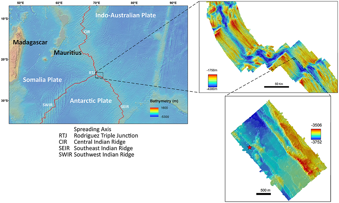
Figure 1. Maps of the study area showing the location of data collection. The red star indicates the vent field in a depth of 3,659 m.
Image Acquisition and 3D Reconstruction
For the video survey the ROV Victor 6000 used a forward looking HD-Camera (3-CCD camera with 1920X1080 pixels) with fixed zoom, pan and tilt, and a pair of lasers (10 cm apart) as scale. The aim of this video survey was to record the megabenthos occurring on the active chimney. The survey was planned and conducted with slow speed during filming (speed over ground ranged approximately between 0.1 and 0.2 knots), an overlap of at least 50 % of each vertical transect line and, if possible, a constant distance toward the chimney walls. The raw imagery data is archived at the data repository Pangea.1
The position of the ROV, its altitude, pitch and roll were logged every second using the “Ultra Short Base Line System” (USBL). The raw USBL positioning was smoothed and interpolated in ArcGIS to remove misallocated positions. The interpolation added a GPS position for each second of which one coordinate was used every 3 s for georeferencing the extracted frame grabs in the 3D reconstruction software. Additionally, the altitude was used for the 3D reconstruction, pitch and roll were not required by the software and the orientation of the imagery was accurate without these parameters.
For the 3D image reconstruction frame grabs were extracted every 3 s from the continuous recorded video imagery using MAGIX Video deluxe 2014 Premium2 and imported in the Pix4D3 software. The Software uses the “Structure from Motion” technique (SfM) to build a 3D image reconstruction of the filmed surface with the preset setting “3D Map” provided by the software. The software was set to the coordinate system WGS84/ UTM zone 42S to match the ROV derived coordinates and set the internal units to meter. The 3D model was scaled and georeferenced by using the smoothed USBL position of every frame grab. Lasers visible in the frame grabs were used to apply scale constraints to optimize scaling and related measurements within the reconstructed model. The USBL and video imagery data was connected using the UTC time. The software allows aerial and distance measurements within the reconstructed textured mesh.
A summary of the reconstruction process is given in Figure 2; a detailed fly through the reconstructed chimney is available in the Supplementary Video 1.
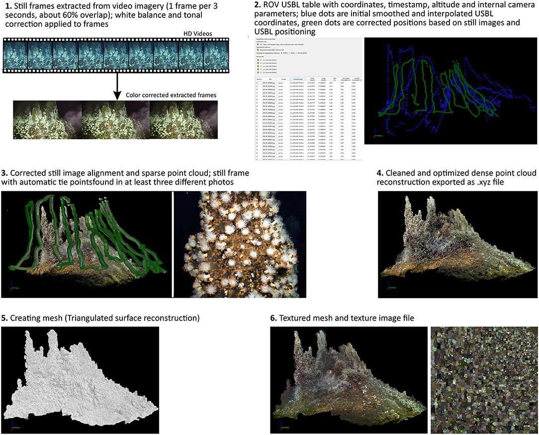
Figure 2. Workflow of the 3D reconstruction from HD video footage to textured mesh.
Terrain Analysis
The point cloud processing software CloudCompare4 was used to calculate the terrain descriptors distance to black and diffuse fluids, aspect, slope, roughness and curvature of the reconstructed chimney model (Figure 3, Table 1). Aspect is the compass direction of the surface. Slope is the vertical gradient of a surface. Roughness is the difference between the minimum and maximum bathymetry values at a given surface area. Curvature measures acceleration, deceleration, convergence and divergence of flow across a surface and therefore indicates areas influenced by erosion or deposition processes. In areas with dense faunal aggregations, the extracted terrain descriptors derived from the surface of these aggregations.
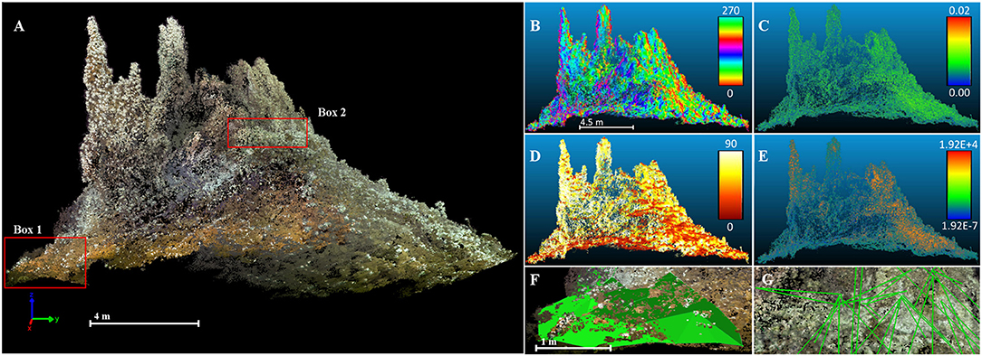
Figure 3. South side of reconstructed 3D textured dense point cloud and derived terrain variables. (A) Textured dense point cloud of the reconstructed chimney. (Box 1) delineates the outline of the extracted frame (F); (Box 2) delineates the outline of the extracted frame (G). All following terrain variables were calculated at a radius of 0.02 m. (B) Aspect of chimney. (C) Roughness. (D) Slope. (E) Gaussian surface curvature. (F) Surface area measurement. Green surface indicates the measured area. (G) Distance measurements to black and diffuse fluids.
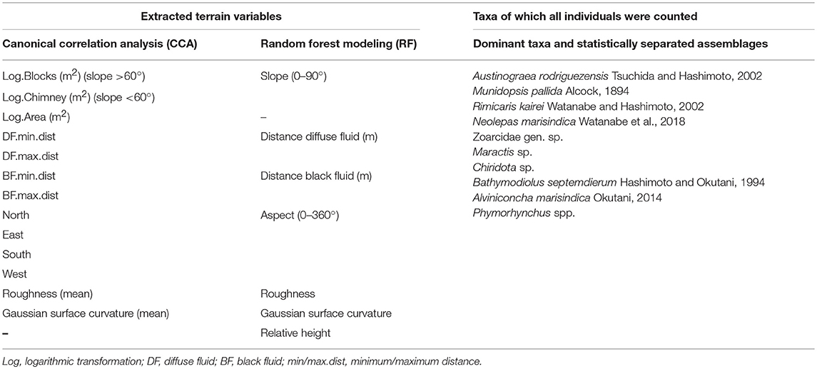
Table 1. Extracted terrain variables used for the Canonical Correlation Analysis (CCA), the Random Forest Modeling (RF) and Taxa of which all individuals were counted for the dominant taxa and statistically separated faunal assemblages.
Diffuse fluid exits were defined by visible, focused and clear fluids, which were indicated by shimmering water, bacterial mats around the exits and the occurrence of vent fauna around these exits. The orientation of the surface of a reconstructed model (normals) was computed for the entire point cloud and converted to dip/dip direction to obtain slope and aspect values.
Based on the resolution of our model all terrain descriptors were calculated at a radius size of 0.02 m to test for small scale changes. The resulting point cloud was exported as asci text file for further analysis in R (R Development Core Team, 2018). In R, the relative height was calculated based on the height of the reconstructed chimney complex model and used as terrain descriptor (Table 1).
Counting Individuals and Definition of Faunal Assemblages
The Pix4D photogrammetry software was used to classify the dense point cloud and assign as separate faunal assemblages based on the underlying 3D textured mesh in combination with the observation of the HD video. The initial classification and assignment of the dense point cloud was based on predominant taxa observed in the video imagery (Table 1).
The extracted and overlapping frame grabs of the video imagery were imported in the web based annotation software BIIGLE (Langenkämper et al., 2017). To ensure the highest imagery quality for counting, the high overlap of the imagery allowed us: a) select only the focused areas within each photo, b) exclude areas of surrounding images and lower resolution parts when individuals were counted. In addition, a taxon-specific colored point was placed on each single individual to avoid double counting.
Of all taxa larger than 2 cm and clearly recognizable throughout the entire video footage, each individual was counted within the reconstructed chimney (Table 1). For taxa that form multilayered aggregations a “minimum abundance” was counted (Marsh et al., 2012), since only the topmost individuals were visible and could be reliably identified.
The identification of taxa within the model was done by a single person and relied on an expert reviewed and sample confirmed imagery catalog, created, and continuously updated since 2011. The identification of taxa throughout the model was cross checked afterwards. The identification catalog is available at the data repository Pangea (doi: 10.1594/PANGAEA.896158).
Faunal assemblages were assigned in two ways. One approach classified faunal assemblages based on the predominant megafauna visible in the video imagery. If taxa were not dominating, geological and bacterial derived visible features were used. The geological description and interpretation applied in this study has been cross checked and confirmed by experienced marine geologists. Abundances were counted in BIIGLE and assemblage borders inspected and cross checked with the 3D reconstruction in Pix4D. In a second approach, a statistical test was applied to define faunal assemblages based on taxonomic richness and abundances (see section “Assemblage analysis” for details).
The abundance data was manually assigned to each faunal patch for all assemblages from the 3D reconstruction classification. Therefore, BIIGLE derived abundance data was aligned with the classified dense point cloud patches and the abundance data was assigned to each faunal patch. The species and abundance data was transformed to abundance per square meter for each taxon and resulted in a single value for each taxon in each individual patch. For all faunal assemblages the mean abundances per square meter of each taxon were calculated. Single individuals were sampled to verify the imagery based identification of all counted taxa at the vent field.
Assemblage Analysis
Dominant Taxa Approach
The faunal assemblage classification based on dominant taxa was statistically tested. Statistically defined indicator species were interrelated to their spatial distribution and assemblage fidelity using the Species-site group association function “IndVal.g” within the “multipatt” package of the “indicspecies” library in R (De Cáceres and Legendre, 2009; De Cáceres et al., 2010). The output is an association value (stat), showing the exclusivity and fidelity of a species for a designated group, which was used to verify the assemblage classification.
To test the assignment of the faunal assemblages, the Bray Curtis dissimilarity matrix of standardized individuals per m2 (ind. m−2) and square root transformed abundance data of all taxa was calculated. The faunal assemblages were displayed as nMDS plot and general assemblage separation was verified using the function “adonis” in R, an equivalent to ANOVA for non-normal and non-homogenous distributed data. Adonis separation of faunal assemblages was based on adjusted p-values with 999 free permutations. The “pairwiseAdonis” package was applied for a pairwise comparison of all faunal assemblages and to show which faunal groups could be significantly separated (Martinez Arbizu, 2017).
Statistical Approach
The statistical assignment of faunal assemblages was done to detect abundance and species richness related delimitations of the fauna occurrences. The k-medoid algorithm “pam” (partitioning around medoids) in combination with the “Adonis” and “pairwiseAdonis” packages were used to analyze and classify the assemblage structure (Maechler et al., 2018). The “pam” clustering algorithm of the k-medoid statistics used Bray Curtis dissimilarity on the transformed matrix to assign a coherent number of faunal assemblages.
The resulting silouhette-plot showed the number of assemblages that could best explain the separation of the species and abundance data (Supplementary Figure 1A). The silhouhette-width plot showed the strength of each faunal patch to belong to the calculated assemblage (Supplementary Figure 1B). The “pam” derived partitioning was tested using the “adonis” function for an overall separation and the “pairwiseAdonis” package to test pairwise separation of faunal assemblages.
The statistically classified faunal assemblages were tested for indicator species as well using the “IndVal.g” function in R (modified after Robert et al., 2014).
Statistical Data Analysis
Abundance data of each faunal patch and terrain variables of the entire reconstructed model were imported into R and formatted to data matrices for further statistical analysis. The Kruskall Wallis test (“stats” package in R) was used to show significant differences in the distances of the faunal assemblages to black and diffuse fluid exits. Dunns test (“dunn.test;” package in R) based on the Benjamini-Hochberg procedure was performed to check for pairwise comparison and separation of the faunal assemblages. The Benjamini-Hochberg procedure is a post-hoc test to adjust the level of significance and reduces false positive errors.
Linear Terrain Variable Analysis
The surface area of the entire model and of each designated faunal assemblage were measured and used for the Canonical-correlation analysis (CCA) that finds maximum correlations of cross-covariance matrices. Minimum and maximum distances to black fluid and diffuse fluid exits were measured as well (Table 1). Measurements were repeated to ensure the minimum or maximum distance. All terrain variables were displayed in scatter plots to visually inspect for the convenience of data transformation. In total, 13 terrain variables were tested to explain the faunal assemblage structure in a CCA (Table 1). Slope values derived from log transformed surface area values and were assigned as vertical chimney area (Log.Chimney) or talus area (Log.Blocks), depending on the steepness (Table 1). Aspect values were split in percentage of faunal patch pointing north, east, south and west (Table 1). This procedure increased the number of terrain descriptors.
The transformed abundance data was tested for a correlation to the terrain data. The “adonis” function was used to find significant terrain descriptors that explain the faunal assemblages and the CCA was repeated using significant factors only. For the CCA analysis, single values for each faunal patch (70 in total) were used, either as mean values or as individual values for distance measurements (Table 1). The terrain variable data set was not the same as for the random forest modeling.
Decision Tree Based Terrain Variable Analysis
The non-linear decision tree model “random forest” was used to find non-linear relationships of assigned faunal assemblages and terrain variables. We created two training data sets with seven extracted terrain variables (predictors) that used 1.00 % of the total data points from the reconstructed point cloud (dense point cloud). These points were extracted randomly throughout the entire chimney complex and contained, besides the terrain variable values, only information to which faunal assemblage the extracted point belongs. Each point had unique terrain variable values.
One training data set extracted data points from the dominant taxa derived faunal assemblages and a second from the statistically relevant derived faunal assemblages. For each data set 5,000 decision trees were built that used all seven terrain variables randomly selected at each node to find a tree best explaining the faunal assemblages. The Out-of-bag error rate (OOB) was estimated and showed misclassifications of the model as well as the minimum number of trees to reduce the variability of the error rate of each tree. The random forest model is significant at an error rate below 5.0 %. The “VarImpPlot” shows the importance of each terrain variable to explain the faunal assemblage structure. The false positive error was calculated for both predictions using the post-hoc test described in Rossel and Martínez Arbizu (2018). If necessary, the Laplace correction was applied on the data prior to the post-hoc test.
A decision tree was obtained from each of the two training data sets. These trees were the foundation for the spatial habitat prediction and have been applied for the entire reconstructed chimney complex, to test the explanation power of the terrain variables.
In contrast to the CCA analysis, the random forest analysis used seven terrain variables (height, aspect, roughness, slope, Gaussian surface curvature, distance to black and diffuse fluids; Figure 3) with individual values for each of the 4,114,358 data points.
Results
3D Reconstruction
It was possible to create a continuous 3D model of one side of the active chimney complex within the hydrothermal vent field. The average resolution expressed as the ground sampling distance has a value of 0.0027 m, sufficient to locate single individuals within the reconstructed model. Highly motile taxa, such as Rimicaris kairei, could not be reconstructed in situ, since they moved too much from image to image and are displayed as a gray area in the model (Figure 4A).
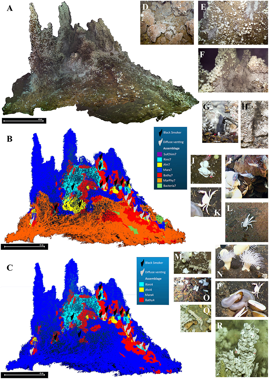
Figure 4. South side structure from motion textured mesh of the 3D chimney reconstruction, detail of the textured surface and manually assigned faunal assemblages. (A) Textured reconstructed chimney. (B) Faunal assemblage distribution assigned by dominant taxa. (C) Faunal assemblage distribution based on k-medoid clustering. (D) Sulfide blocks of the chimney complex. (E) Overview of mussel and shrimp aggregations. (F) Overview of shrimp and anemone aggregations. (G) Diffuse fluid exit. (H) Black fluid exit. (I) Phymorhynchus spp.. (J) Rimicaris kairei. (K) Austinograea rodriguezensis. (L) Munidopsis pallida. (M) Neolepas marisindica. (N) Maractis sp.. (O) Bathymodiolus septemdierum. (P) Chiridota sp.. (Q) Zoarcidae gen. sp.. (R) Alviniconcha marisindica.
The smoothed USBL positioning had an absolute standard deviation error of 1.8 m for the x-direction, 2.0 m for the y-direction and 1.3 m for the z-direction, which was below the expected USBL error rates of 1 % (40 m); the computed scale constraint error length was 0.023 m. The initial input camera parameters differed 12.64 % compared to the optimized internal camera parameters from the SfM reconstruction.
Geological Setting of the Chimney Complex
The base of the chimney complex consisted of superficially oxidized sulfide talus blocks and chimney fragments in size ranges of 5–40 cm and had a moderate slope (5–40°); the upper part had continuous solid and often oxidized surfaces with a steep to vertical slope ranging from 50–90°.The western side of the reconstructed chimney was relatively shallow at the base and rose abruptly into the vertical chimney structure. The eastern side had an almost continuous slope that became steeper in the upper part, with more active diffuse and black fluid venting zones (Figures 4B,C). The intact upstanding chimneys were invariably inactive.The diffuse venting occurred in the lower part of the chimney complex, the black fluid exits were all located at intermediate heights.Sulfidic sediments, sulfide rubble, or gravel occurred infrequently, while no basaltic rocks of any size or biogenic sediments were observed.
Taxonomic Composition
Ten different taxa with a total abundance of 25,360 individuals and a density range of 0.01–23.59 individuals per m2 (ind. m−2) among different taxa could be recognized reliably throughout the entire chimney complex (Table 2). The abundance per square meter is averaged over the entire reconstructed chimney area.
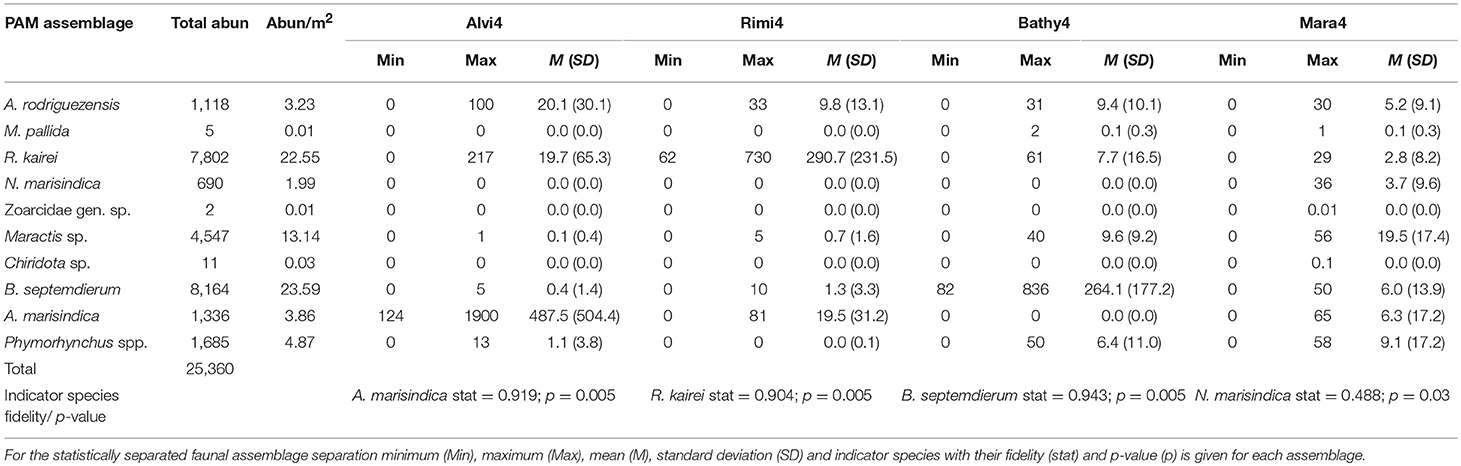
Table 2. All morphotypes or species and their total and per square meter abundances within the entire chimney.
These ten taxa were ordered in decreasing abundance (Table 2) and comprised the mussel Bathymodiolus septemdierum Hashimoto and Okutani, 1994 (Figure 4O), the shrimp Rimicaris kairei (Figure 4J), the anemone Maractis sp. (Figure 4N), the gastropods Phymorhynchus spp. (Figure 4I) and Alviniconcha marisindica Okutani, 2014 (Figure 4R), the crab Austinograea rodriguezensis (Figure 4K), the stalked barnacle Neolepas marisindica (Figure 4M), the holothurian Chiridota sp. (Figure 4P), the squat lobster Munidopsis pallida Alcock, 1894 (Figure 4L) and a hydrothermal fish of the family Zoarcidae gen. sp. (Figure 4Q).
Bathymodiolus septemdierum, Maractis sp., Phymorhynchus spp., A. marisindica and N. marisindica are species that form aggregations, of which B. septemdierum, N. marisindica and Maractis sp. are non-motile or restricted in their ability to move. Bathymodiolus septemdierum, R. kairei and A. marisindica are symbiotic taxa bearing either endosymbiotic or episymbiotic bacteria. Accordingly, these taxa were related to the fluid distances and dominant visible taxa changed from A. marisindica to R. kairei and A. rodriguezensis to B. septemdierum to Maractis sp. with increasing distance (compare Figures 5A,B with Figures 5C,D). The distances to black fluid exits were thereby more pronounced compared to distances to diffuse fluid exits (compare Figures 5C,D with Figures 5E,F).
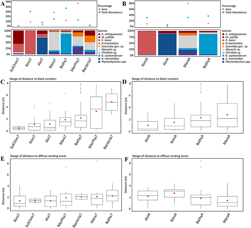
Figure 5. (A,C,E) show the results of the seven dominant taxa based assemblage separation and the figures (B,D,F) show the results of the four statistically separated faunal assemblages. (A,B) Upper part: Percentage of total area of each faunal assemblage type and the total proportional abundance of each faunal assemblage. Lower Part: Proportion of taxa occurring in each faunal assemblage. (C,D) Range of distance of each faunal assemblage to black fluid exits. (E,F) Range of distance of each faunal assemblage to diffuse fluid exits.
Further taxa have been observed or were sampled but could not be reliably recognized throughout the entire chimney complex. All occurring taxa and their affiliation to faunal assemblages are listed in Supplementary Table 1.
Faunal Assemblages
Point cloud assemblage assignments based on the reconstructed textured mesh were verified by imagery (Figures 4D–F). The dominant taxa approach defined faunal assemblages based on dominant visible taxa and was confirmed by identifying indicator species. The statistical approach used k-medoid clustering to define the number of clusters with lowest intra-cluster variance and highest inter-cluster variance (Supplementary Figure 1), confirmed by “pairwiseAdonis” comparison.
Dominant Taxa Assemblage Assignment
The dominant taxa approach identified seven faunal assemblages (Figure 4B), named SulChim7, Rimi7, Alvi7, Mara7, Bathy7, MarPhy7, and Bacteria7, which were supported by indicator species analysis. It designates R. kairei (stat = 0.9; p = 0.005) as indicator species for the faunal assemblages SulChim7 and Rimi7. Alviniconcha marisindica occurs in assemblage Alvi7 (stat = 0.929; p = 0.005), B. septemdierum (stat = 0.915; p = 0.005) is related to the Bathy7 assemblage. The species Phymorhynchus sp. (stat = 0.786; p = 0.02) occurs in the faunal assemblages Mara7, Bathy7, MarPhy7, Bacteria7 and SulChim7. Maractis sp. (stat = 0.883; p = 0.005) occurs in the assemblages Mara7, Bathy7, MarPhy7, Bacteria7, and SulChim7.
Species related to more than one faunal assemblage either occurred in close proximity to fluid exits throughout different assemblages or in certain distances to fluid exits, and often had varying abundances or individual sizes. The “pairwiseAdonis” comparison of each faunal assemblage could significantly distinguish the assemblages close to fluid exits from those further away of fluid sources, but not every assemblage could be separated from one another (Supplementary Table 2).
Statistical Assemblage Assignment
The statistical faunal assemblages based on k-medoid clustering suggested a separation in four assemblages (Figure 4C). This could best explain the species and abundance data with an overall silhouette value of 0.44 (Supplementary Figure 1A). The silhouette- width plot showed that the majority of the faunal patches fit to the newly defined assemblages (Supplementary Figure 1). The Mara4 assemblage has a silhouette width of 0.50 and consists of 21 faunal patches; the Rimi4 assemblage has a silhouette width of 0.31 with 9 faunal patches, the Bathy4 assemblage has 29 faunal patches with a silhouette width of 0.46 and the Alvi4 assemblage has a silhouette width of 0.37 with 11 faunal patches. All newly defined faunal assemblages could be significantly separated using the “pairwiseAdonis” comparison (Supplementary Table 2).
Comparing Dominant Taxa and Statistically Defined Faunal Assemblages
The statistical k-medoid clustering resulted in an extension of the Mara4 assemblage, incorporating Mara7, MarPhy7, and Bacteria7 based on similar taxa and abundances. Similarly, several patches of the Bathy7, Alvi7, and SulChim7 assemblages changed to Mara4.
Indicator species for each group also changed with Neolepas marisindica representing Mara4 (stat = 0.488; p = 0.03), R. kairei the Rimi4 assemblage (stat = 0.904; p = 0.005), B. septemdierum the Bathy4 assemblage (stat = 0.943; p = 0.005) and A. marisindica the Alvi4 assemblage (stat = 0.919; p = 0.005). The taxon Maractis sp. could be related to the combined Mara4 and Bathy4 assemblages (stat = 0.859; p = 0.005).
The distribution of the seven dominant taxa and the four statistically identified assemblages showed similar patterns. Close to fluid exits, relatively higher abundances over similar spatial scales were observed compared to assemblages further away, that occupy more space, but these findings were not statistically supported (compare Figures 5A,B with Figures 5C,D).
The alterations of the faunal patches belonging to the seven and four faunal assemblages were visualized in nMDS plots based on the Bray Curtis dissimilarity (Figures 6A,B). The seven faunal assemblages could be significantly separated from several, but not all, other assemblages (Supplementary Table 2A). Nevertheless, the Alvi7, Rimi7, and Bathy7 assemblages form consistent clusters, but Bacteria7, Mara7, MarPhy7, and SulChim7 could not be separated and show large overlap (Figure 6A). In contrast, the statistically defined four faunal assemblages could be significantly separated from each other (Supplementary Table 2B). Except for some patches of Mara4, no mixing or overlapping of faunal patches occurred (Figure 6B).
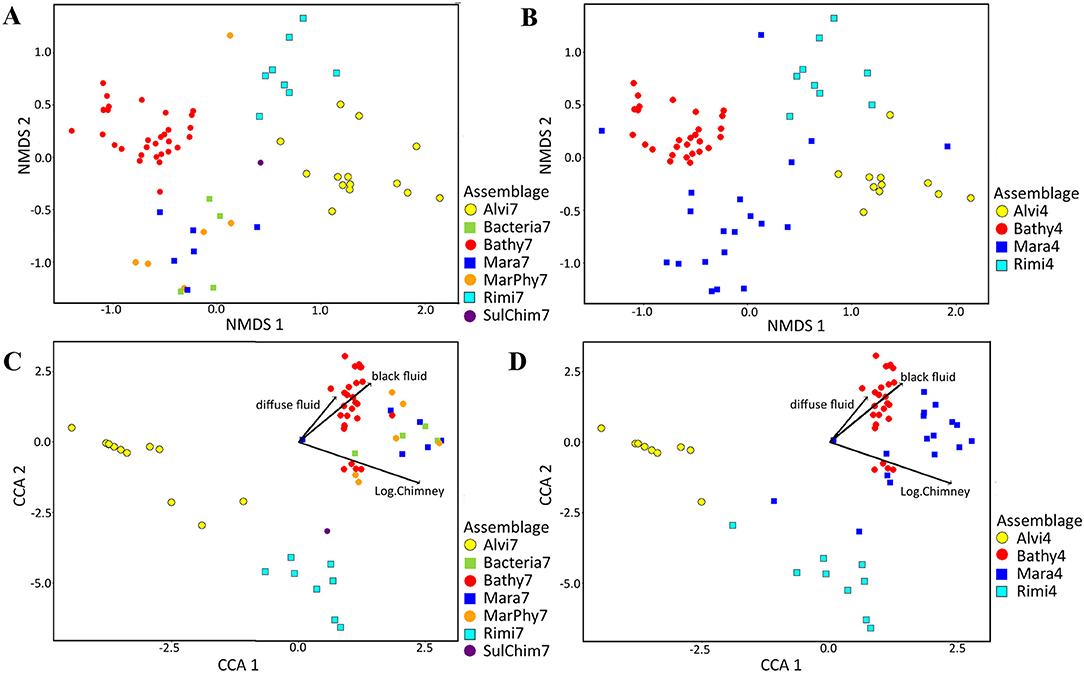
Figure 6. NMDS plots of abundance and species based assemblage structure and CCA plots showing species and abundance distributions in relation to significant terrain variables. Abundance data was square root transformed and Bray Curtis dissimilarity was calculated for all figures. In total, 13 terrain variables were tested for their influence for the assemblage separation of which three variables were a priori log transformed (chimney area, sulfide block area and assemblage area). (A) Taxonomic based nMDS plot with seven faunal assemblages (Stress = 0.12512). (B) nMDS plot with four faunal assemblages (Stress = 0.12512). (C) Canonical correspondence analysis (CCA) using the Bray Curtis dissimilarity matrix for combination of abundance based faunal assemblage separation and its relation to terrain variables for seven faunal assemblages. (D) CCA analysis with four assemblages.
Linear Modeling of the Ecological Spatial Pattern
The dominant taxa based seven faunal assemblages and statistically defined four faunal assemblages were tested for terrain variables being responsible for their distribution (Figures 6C,D). Thirteen terrain variables were used for the CCA (Table 3), of which, factors “Log.Blocks (m2)”, “Log.Chimney (m2)”, and “Log.Area (m2)” were log-transformed prior to the analysis. All abiotic factors could explain 29.69 % of the variability of both faunal assemblages.
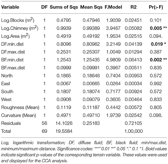
Table 3. Significance value derived from the permutational multivariate analysis of variance (adonis) of all used terrain variables.
Using only the three significant factors based on “adonis” analysis (Table 3), 13.49 % of the assemblage structure could be explained (Figures 6C,D). These factors were the log-transformed vertical chimney area, as well as the minimum distances to diffuse- and black fluids (Table 3).
Bathy7, Bacteria7, Mara7, and MarPhy7 were positively correlated with the significant terrain variables (Figure 6C), meaning they occurred in greater distances to black and diffuse fluids and occupied more vertical chimney space. The faunal assemblage Bathy7 could be separated statistically and the majority of its patches had strong correlations with the distance to black and diffuse fluids.
The faunal assemblages Rimi7 and Alvi7 occurred closer to diffuse and black fluids. Rimi7 depends more on vertical structures and could thereby be separated from Alvi7 (Figure 6C). The statistically reduced number of faunal assemblages indicated similar correlations to terrain variables for Rimi4, Alvi4, and Bathy4 (Figure 6D). The overlapping Bacteria7, Mara7, and MarPhy7 assemblages were merged into Mara4 and are depending on a greater distance to diffuse- and black fluids according to the CCA analysis.
Random Forest Modeling of the Ecological Spatial Pattern
The random forest modeling explored the explanation power of key terrain variables responsible for the faunal assemblage distribution pattern. The training data and prediction of the faunal assemblages relied on abiotic terrain variables only, with species richness and abundances being excluded.
The random forest model of the dominant taxa assemblage had an estimated OOB error rate of 24.73 %, and the statistically defined assemblage model had an error rate of 14.96 %. In both models the most important terrain variables were distances to black- and diffuse fluids and the height of the chimney complex (Supplementary Figure 2). Roughness, aspect, slope and curvature were of minor importance. The resulting decision trees were used with all terrain variables for the prediction of all faunal assemblages (Figure 7).
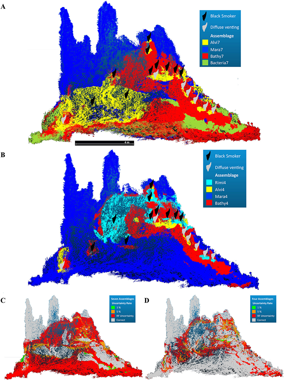
Figure 7. Predicted faunal assemblage occurrence across the reconstructed chimney complex based on random forest modeling. (A) Occurrence of the seven faunal assemblages based on the winning classes of the predicted random forest model (Accuracy = 0.4405). (B) Occurrence of the four faunal assemblages based on the winning classes of the predicted random forest model (Accuracy = 0.8497). (C,D) False positive uncertainty rate at 1%, 5% and the random forest prediction uncertainty for both assemblages.
The random forest prediction for the dominant taxa assemblages could assign Mara7, Bathy7, and Alvi7 with a total accuracy of 44.05 % (Figures 7A,C), while Rimi7, MarPhy7, and SulChim7 were not predicted.
MarPhy7 and Bathy7 both occurred close to diffuse venting zones and were represented by the same indicator species (Maractis sp.) for these assemblages. The predicted spatial extent of Bathy7 covered the originally defined Bathy7 and extended into the MarPhy7 assemblage, which was not predicted. Further parts of the initial MarPhy7 assemblage were replaced by the predicted Alvi7, which was predicted far beyond its original occurrence (compare Figures 4B, 7A). The Bacteria7 assemblage was predicted as coherent patches and scattered within the initially defined MarPhy7 or Bathy7 extent.
The random forest prediction for the statistically defined faunal assemblages could assign all assemblages with a total accuracy of 84.97 % (Figures 7B,D). All faunal assemblages were correctly predicted with only minor spatial differences at the transitions (Figure 7D).
The predicted Mara4 assemblage occurred in comparable spatial extent of the originally classified assemblage. The Bathy4 assemblage was predicted circular around vent fluid effluents with the second largest aerial extent. Rimi4 and Alvi4 had the smallest spatial extent and occurred in close proximity to vent effluents of both types. Predicted Rimi4 patches in greater distances to fluid exits were slightly scattered and confused with Mara4, indicating the importance of the distance of fluid exits to assign this assemblage (Figure 7D). Within the predicted Mara4 and Bathy4 assemblages, the highest classification error rates occurred (Supplementary Table 3B). Nevertheless, all four predicted assemblage occurrences persisted in areas which were statistically classified. The type of fluid exit seemed to be of minor importance, although Rimi4 occurred closer to black fluid exits and Alvi4 closer to diffuse fluids (Figure 7B).
It was observed that slope, curvature and roughness were more pronounced in close proximity to fluid exits. In both predictions the structuring terrain variables were comparable to the “adonis” derived terrain variables of the CCA analysis.
Discussion
Faunal Assemblage Reduction
The definition of faunal assemblages based on dominant visible taxa has been commonly used in many imagery studies (Sarrazin et al., 1997; Cuvelier et al., 2009; Marsh et al., 2012) and is still the basis to outline occurrences of single taxa that often do not overlap in their spatial extent (Podowski et al., 2009; Sen et al., 2013; Thornton et al., 2016). While the use of statistical methods to define faunal assemblages is robust, reproducible and can be applied for unknown areas (Vierod et al., 2014; Robert et al., 2016; Fernandez-Arcaya et al., 2017), the dominant taxa approach offers the advantage to include biological observations such as foraging stage or individual sizes (Cuvelier et al., 2009; Marsh et al., 2012), which might be overlooked when relying on statistical methods only.
Including observations such as individual size, foraging information, motility or feeding mode in a statistical assemblage definition approach leads toward functional trait analysis and yields different explanations such as functional group structure (Vierod et al., 2014; Gagic et al., 2015; Shojaei et al., 2015) or recovery and resilience potential (Gollner et al., 2017). This requires a basic knowledge about the taxonomic composition and assemblage structure.
In our study, the reduction from seven dominant taxa based assemblages to the four statistically identified faunal assemblages was related to similarities in taxonomic and abundance composition within different faunal patches. The Mara7 and MarPhy7 assemblages for example had a similar assemblage structure, but taxa such as Maractis sp. occurred in lower abundances within the MarPhy7 assemblage. In addition, close to fluid exits, individuals were larger than further away of fluid exits. These differences were recognized and resulted in more assemblages for the dominant taxa based approach, but was not supported statistically (Figure 6A).
These abundance and size differences might be related to feeding and aging but were neither reflected in the biological faunal assemblage classification nor in the terrain variable prediction. Rimicaris kairei as one of the major food sources located around fluid exits (Van Dover, 2002) and the limited space along chimney walls puts a high intraspecific competition pressure on Maractis sp. to settle close to this food source, and individuals occur in dense aggregations at active chimney complexes as observed for Kiwa tyleri at the E2 and E9 vent fields in the Southern Ocean (Marsh et al., 2015). The competition also might inhibit the settlement of offspring and therefore smaller individuals are forced to settle at greater distances as observed for individual sizes of Bathymodiolus azoricus at Lucky Strike vent field (Cuvelier et al., 2011) or the population structure of K. tyleri at the E2 and E9 vent fields in the Southern Ocean (Marsh et al., 2012, 2015).
Although we are aware that minor differences between some faunal patches do exist, we only discuss the statistically defined four faunal assemblages in the following sections.
Faunal Assemblage Characterization and Spatial Distribution
Taxonomic Resemblance
The taxa identified at the chimney complex on the southeast Indian Ridge resemble taxa of Kairei, Edmond, Dodo, and Solitaire vent fields (Van Dover et al., 2001; Nakamura et al., 2012). In total, 17 megafauna taxa have been identified either by video data or molecular confirmed samples.
Ten species are in common with vent fields on the Central Indian Ridge (CIR), the South West Indian Ridge (SWIR) and the South East Indian Ridge (SEIR).
The shrimp Rimicaris kairei, three species of the gastropod Phymorhynchus spp., two species of the limpet Lepetodrilus spp. and the squat lobster Munidopsis sp. (Van Dover et al., 2001; Nakamura et al., 2012; Copley et al., 2016), are known from all Indian Ocean vent sites, with Munidospsis spp. having a panoceanic distribution (Copley et al., 2007; Sen et al., 2013). The gastropod Chrysomallon squamiferum was observed throughout the Indian Ocean except at Dodo vent field in the northern CIR (Chen et al., 2014). The mussel Bathymodiolus spp., referred to as Bathymodiolus sp. at Dodo and Solitaire vent field (Nakamura et al., 2012) and B. marisindicus Hashimoto, 2001 at Longqi (Copley et al., 2016), Kairei and Edmond vent fields (Breusing et al., 2015) occurred on the SWIR and CIR and shows a historic connectivity with Bathymodiolus spp. in the western Pacific (Breusing et al., 2015). The stalked barnacle Neolepas marisindica, which has been recently described for the SEIR (Watanabe et al., 2018), is the same species at Kairei (Hashimoto et al., 2001) and Longqi (Copley et al., 2016).
The anemone Maractis sp. (Van Dover et al., 2001; Copley et al., 2007) (referred as Marianactis sp. at other vent sites), the gastropod Alviniconcha marisindica (Hashimoto et al., 2001), the crab Austinograea rodriguezensis (Van Dover et al., 2001, Nakamura et al., 2013), the shrimps Mirocaris indica Komai et al., 2006 (Komai et al., 2006) and Alvinocaris solitaire Yahagi et al., 2014 (Van Dover, 2002) are found only at certain Indian Ocean sites. The hydrothermal holothurian Chiridota sp. (Van Dover et al., 2001) and the hydrothermal fish Zoarcidae gen. sp. (Ingole, 2003) are known from the Indian Ocean but are probably new species, the latter one a new genus of fish.
These 17 taxa are within the range of 4 to 35 taxa observed at vent fields on the CIR and the SWIR (Van Dover et al., 2001; Nakamura et al., 2012; Copley et al., 2016).
Alvi4 Assemblage
Large aggregations of Alviniconcha marisindica and Austinograea rodriguezenis occurred in the Alvi4 assemblage, nearby black fluid effluents. This spatial distribution is comparable to the Eastern Lau Spreading Center (Podowski et al., 2010; Sen et al., 2013) or Solitaire vent field (Nakamura et al., 2012), where gastropods of the genus Alviniconcha were observed close to black fluid effluents, in contrast to Kairei vent field, where they occurred around diffuse fluid exits (Hashimoto et al., 2001).
Alviniconcha marisindica is a symbiotic species bearing sulfide-oxidizing bacteria in its gills, therefore benefiting of the close proximity to hydrothermal fluids (Van Dover, 2002). This taxon can be found exclusively in closest proximity to fluid exits and in highest measured temperature anomalies within a vent field (Podowski et al., 2010; Sen et al., 2013).
No direct comparison of this abundance was possible, since the spatial coverage of Alviniconcha spp. is often used as surrogates for their dominance at vent fields (Sen et al., 2013, 2014; Du Preez and Fisher 2018). Alviniconcha sp. often occurs in dense and multilayered aggregations (Sen et al., 2014) hampering exact abundance estimates, although this has been done for aggregated and multilayered taxa such as Kiwa tyleri (Marsh et al., 2012) or R. kairei (Connelly et al., 2012). Counting aggregated species always estimates a so called “minimum abundance” of the superficial layer of individuals (Marsh et al., 2012); a different approach calculates the surface area and applies mean individual sizes (Podowski et al., 2009), which requires representative sampling and measuring.
Rimi4 Assemblage
The Rimi4 assemblage followed Alvi4 in terms of fluid proximity and is dominated by Rimicaris kairei with high abundances in dense and multilayered aggregations around major black fluid exits. This value is almost 4-fold higher than the maximum abundance at Iheya North field in the Okinawa Through but lower compared to Von Damm and Beebe vent field with one third of the individuals at the Mid-Cayman spreading center (Connelly et al., 2012; Thornton et al., 2016). The low maximum abundances at Iheya North field might be related to small patch sizes of the alvinocaridid aggregations in contrast to multilayered occurrences at Mid-Cayman spreading center or presented here.
Abundance data for Kairei, Edmond, Solitaire, and Dodo vent fields are not reported (Hashimoto et al., 2001; Van Dover et al., 2001; Nakamura et al., 2012), so here we present the first quantitative abundance estimation for the Indian Ocean biogeographic province.
Rimicaris kairei was always found close to fluid exits, up to a distance of a few meters away, comparable to Kairei vent field (Van Dover, 2002). Alvinocaridid shrimps are suggested to indicate vent fluid exits (Cuvelier et al., 2009; Ishibashi et al., 2015) and often represent the dominant taxon closest to vent effluents (Van Dover et al., 1996; Desbruyères et al., 2001; Van Dover, 2002; Watabe and Hashimoto, 2002; Meyer and Paulay, 2005; Connelly et al., 2012).
Rimicaris kairei is a symbiotic species suggested to feed entirely on sulfide-oxidizing bacteria in their branchial chambers as adults (Van Dover, 2002; Watabe and Hashimoto, 2002), explaining their proximity to vent fluid exits. Their occurrence in water temperatures above 10°C indicate a high thermal tolerance and supports this idea (Van Dover, 2002; Fabri et al., 2011).
Further taxa within this assemblage were randomly distributed single individuals of A. marisindica and the bythograeid crab A. rodriguezensis.
Bathy4 Assemblage
Within the Bathy4 assemblage Bathymodiolus septemdierum occurred in dense aggregations, comparable with densities observed at Minami-Ensei Knoll and Iheya North field, both located at the Okinawa Through (Fujikura et al., 2002; Thornton et al., 2016).
These high abundances of B. septemdierum were observed close to diffuse fluids and in moderate distances to black fluids, as reported for B. marisindicus at Longqi vent field (Copley et al., 2016), at Kairei vent field (Hashimoto et al., 2001; Van Dover et al., 2001), and comparable with Bathymodiolus platifrons Hashimoto and Okutani, 1994 and B. japonicus at Iheya North vent field (Thornton et al., 2016).
Bathymodiolus mussels are known as symbiotic species containing thiotrophic bacteria on their gills (Goffredi et al., 2004) that are likely acquired from their surrounding habitat (Thomas et al., 2018). Its individual composition can be highly variable within a single vent site (Van Dover, 2002). Some mussels contain methanotrophic symbionts or a mix of thio- and methanotrophic bacteria (Pond et al., 1998; De Busserolles et al., 2009). Despite their symbiotic ability, they are mixotrophic and remain a functional gut and filter feeding habit (Thomas et al., 2018), which could be related with a lower temperature tolerance (Podowski et al., 2009) and their preference to form greater aggregations on basaltic surfaces (Podowski et al., 2010).
Mussels of the genus Bathymodiolus are founder species that structure the community (Gollner et al., 2015; Du Preez and Fisher, 2018) and increase community dynamics (Breusing et al., 2015; Ferrigno et al., 2017). In accordance with findings of Sen et al. (2014), the Bathy4 assemblage had the highest total abundance of all faunal assemblages (Table 2), despite not covering the largest surface area (Figure 5B). It should be kept in mind, that only the “minimum abundance” of this aggregation forming species was counted.
Further associated and quantified species are A. rodriguezensis, R. kairei, Phymorynchus sp. and Maractis sp., of which A. rodriguezensis, R. kairei and Phymorhynchus sp. had smaller sizes. The Phymorhynchus gastropod, also found in Bathy4, often occurred in small aggregations as observed at Longqi vent field (Copley et al., 2016). In addition, the squat lobster Munidopsis pallida was observed, a species that is usually found in the periphery of vent fields with little or no venting (Podowski et al., 2010; Sen et al., 2014).
Mara4 Assemblage
The Mara4 assemblage was the most diverse faunal assemblage with ten different taxa, of which six occurred in their highest abundances. These taxa were Maractis sp., Phymorhynchus sp., N. marisindica, M. pallida, Chiridota sp. and the zoarcid fish. Further taxa were A. rodriguezensis, R. kairei, B. septemdierum, and A. marisindica in slightly lower abundances compared to their occurrences in other faunal assemblages (Table 2).
The maximum abundances of Maractis sp. are comparable with abundances at Tow Cam vent field at the Eastern Lau Spreading Center in the Pacific Ocean (Podowski et al., 2010) and one and a half fold higher compared to abundances at Ashadze vent field from the MAR (Fabri et al., 2011), or at the E9 vent field in the Southern Ocean (Marsh et al., 2012). Slightly lower abundances were reported for the Beebe vent field at the Mid-Cayman spreading center in the Caribbean Sea (Connelly et al., 2012) or at TAG hydrothermal mound at the MAR (Copley et al., 2007).
The diversity of the Mara4 assemblage could be the result of mixing vent endemic, non-symbiont reliant or not solely reliant species, such as A. rodriguezensis or B. septemdierum, in lower abundances, with filter feeding, carnivorous and scavenging taxa to form this peripheral community (Fabri et al., 2011; Sen et al., 2016; Goffredi et al., 2017). It has been suggested that anemones can tolerate low levels of hydrothermal fluids and temperatures, which has been measured for M. rimicarivora with a maximum tolerance of 25°C at Ashadze vent field on the MAR (Fabri et al., 2011). They also benefit from the local enhanced availability of potential prey (Podowski et al., 2010), such as R. kairei (Van Dover, 2002) or Kiwa tyleri in the Southern Ocean (Marsh et al., 2012), and this mixed food supply deriving from vent field inorganic carbon production and photosynthetically organic particulates likely support all taxa within this assemblage (Sen et al., 2016). Within the Mara 4 assemblage, highly reproductive species such as R. kairei and provannid gastropods are absent. These taxa might inhibit the settlement of sessile taxa as suggested for anemones closer to vent effluents (Sen et al., 2016).
In addition, close to faunal assemblages with a high total abundance of mobile taxa at black fluid exits, we observed larger sizes of Maractis sp. (Figures 4A,F) as reported for Ashadze vent field on the MAR (Fabri et al., 2011). Especially at vertical chimney structures above black- and diffuse fluid exits, larger individuals were recognized but we did not test for significance. These areas are influenced by hydrothermal fluids with high temperatures and low oxygen levels (Beauchamp et al., 1984; Podowski et al., 2010), but may resemble submarine canyon conditions with vertical cliffs and overhangs, which provide exposed structures, suitable for sessile, and filter feeding anemones (Ferrigno et al., 2017).
Assemblage Structure Implications
Large sulfide deposits, many inactive chimneys and frequently occurring diffuse fluid exits are indications for long lasting activity (Nakamura et al., 2012; Copley et al., 2016). Similarly, decreasing abundances of Alviniconcha spp. and R. kairei were recognized and have been interpreted as proxies for late faunal succession stages (Nakamura et al., 2012; Sen et al., 2014; Du Preez and Fisher, 2018). The shrimps usually establish during early succession stages in dense aggregations as reported for Alvinocaris longirostris Kikuchi and Ohta, 1995 at Iheya North vent field (Nakajima et al., 2015).
Mussel aggregations on the other hand increase during later succession stages and could be stable over time scales of decades (Lessard-Pilon et al., 2010). Bathymodiolus spp. are not observed at the artificially created Iheya North field after a period of 40 months (Nakajima et al., 2015) and this species seems to prefer areas of diffuse flow (Podowski et al., 2009) which might increase at waning vent fields. Additionally, scavengers such as Phymorhynchus sp., hydrothermal holothurians and squat lobster were frequently observed. During waning succession stages, increasing abundances have been reported for Phymorhynchus sp. at Longqi vent field (Copley et al., 2016), for Chiridota hydrothermica Smirnov and Gebruk, 2000 and Munidopsis lauensis Baba and de Saint Laurent, 1992 in the Eastern Lau Spreading Center (Sen et al., 2014). The close proximity of this peripheral community to vent exits might also suggest a waning succession stage, replacing the symbiotic community (Fabri et al., 2011).
Based on these observations we believe that the vent field is rather stable with a slowly changing faunal assemblage dynamic as found at medium spreading rate back-arc basins, where the hydrothermal environment has been observed to be stable for over a decade (Levin et al., 2016a; Gollner et al., 2017; Du Preez and Fisher, 2018).
3D Reconstruction and Terrain Variable Extraction
Mapping structural complex habitats based on 3D reconstructions is a novel technique recently applied at vent fields and submarine canyons to investigate vertical structures, overhangs and horizontal seafloor areas, which is not possible using traditional geographic information systems or 2D mosaics (Thornton et al., 2016; Robert et al., 2017).
The 3D reconstruction in our study successfully combined the analysis of horizontal and vertical imagery in a single dataset that has been separately done in 2D mosaics within vent fields either for vertical chimneys (Cuvelier et al., 2009; Sen et al., 2013) or from a nadir view to map the vent field seafloor surface (Podowski et al., 2009; Fabri et al., 2011). The 3D approach allows the reconstruction of entire vent fields from the periphery to its vertical chimney complexes to obtain high resolution biotic and terrain variable information and address questions of faunal spatial distribution (Thornton et al., 2016), succession patterns (Du Preez and Fisher, 2018) and faunal zonation (Marsh et al., 2012).
An advantage of the SfM technique is its application to any video imagery, without requiring designated video transects. Therefore, even after a natural or anthropogenic disturbance event has taken place it might be possible to get information of the former undisturbed environmental status if any video imagery for this area is available.
In addition, optical images do offer high levels of detail that are easily interpreted by humans (Pizarro et al., 2009). Test trials regarding the resolution showed that 3D reconstruction models can produce reasonable estimates of underwater areas with an error rate of 2 % at a 1cm scale (Pizarro et al., 2009).
Here we present high resolution SfM reconstruction of a highly complex habitat with a diverse faunal composition. We achieved a resolution below 1 cm per pixel. Fine scale physical and geological variables are difficult to detect especially in remote places, where often no terrain variable data is available (Vierod et al., 2014), while directly influencing species and faunal assemblage distributions (Fernandez-Arcaya et al., 2017; Bargain et al., 2018).
Beside vent fluid exposure, further terrain variables could be structuring the spatial distribution of vent species (Goffredi et al., 2017; Bargain et al., 2018), which is difficult to address with 2D imagery. By using 3D techniques we are able to increase the information derived from imagery studies (Friedman et al., 2012) and even terrain variables obtained from 2D mosaics can be gathered with higher precision with regards to distortions that derive when 2D mosaics are created from structurally complex surfaces (Singh et al., 2007).
In the context of potential mining and subsequent anthropogenic activities, causing unintended damages to these ecosystems (Davies et al., 2007; Fernandez-Arcaya et al., 2017), the use of video imagery is a noninvasive technique to analyze this ecosystem. These baseline studies show an undisturbed environmental state of active vent fields and can be used as ground truthing for prospective monitoring work and marine management (Levin et al., 2016b; Robert et al., 2016). Imagery based monitoring can detect and define faunal assemblages before, during and after mining or similar disturbance events and are suggested as cost effective methods (Van Dover et al., 2014; Boschen et al., 2015). Similar work with lower resolution imagery has been done at seamounts after trawling occurred, which shows changes in megafauna (Gollner et al., 2017).
Habitat Prediction Model
Random Forest Model
The linear model could separate the faunal assemblages, but insufficiently explained faunal assemblage distributions across the reconstructed chimney complex (Figures 6C,D). Therefore, nonlinear random forest model was applied and predicted the faunal assemblage structure with an accuracy of 84.97 % (accuracy of each assemblage in Supplementary Table 3).
The random forest model was not significant, this could have been due to the scale of terrain variables. Habitat prediction models for marine canyons pointed out the importance of comparing different scales for each variable (Robert et al., 2015, 2016, 2017; Bargain et al., 2018), which has not been done for our model. We focused on the smallest applicable scale for all terrain variables to show the maximum possible resolution derived from the reconstructed model and several studies pointed out the importance of high resolution small scale data to increase the prediction power of a model (Robert et al., 2015, 2016). Maps created at larger scales often show higher discrepancies between modeling techniques (Robert et al., 2016), as well as between observed and modeled distributions. The use of different scales for the prediction might explain some of the remaining 15 %. Nevertheless, with our high resolution model and smallest applicable terrain variable scale, a major proportion of the faunal assemblage structure was successfully explained.
The low misclassification error and the high prediction accuracy indicated a good performance of the random forest model (Supplementary Table 3). Random forest prediction is supposed to perform better for species richness and diversity, rather than for abundance, (Knudby et al., 2010) and is less affected by prevalence compared to linear models (Robert et al., 2016). Therefore, the use of linear models for data exploration and random forest for prediction has been recommended (Baccini et al., 2004; Robert et al., 2015). This turned out to be valid for our model as well with CCA analysis and random forest prediction resulting in the same significant terrain variables.
In terms of performance, applied predictions at submarine canyons showed that the use of random forest models achieved similar results (Robert et al., 2014; Bargain et al., 2018) or even outperformed linear and non-linear prediction models if compared directly (Robert et al., 2015) as seen in this study.
Structuring Terrain Variables
We were able to identify key structuring factors that were extracted from the high resolution model, of which distance to vent fluids best explained the spatial distribution pattern of the faunal assemblages. This result was promoted by both, the CCA analysis and the random forest model (Figures 6D, 7B).
Specific minimum and maximum distances for vent endemic species have been observed in several studies, often in a concentric distribution around active venting chimneys (Van Dover et al., 1996; Podowski et al., 2010; Fabri et al., 2011; Marsh et al., 2012; Boschen et al., 2016). Additional measurements of physiological tolerances, such as temperature, oxygen and hydrogen sulfide availability revealed a relationship of these physicochemical parameters and the spatial distribution at vent fields (Copley et al., 2007; Schmidt et al., 2008).
However, it remained unclear, whether only fluid distance or further terrain variables, such as exposed vertical structures, terrain roughness or availability of hard substrates were affecting the species occurrences as observed in submarine canyon studies (Vierod et al., 2014; Mascle et al., 2015; Fernandez-Arcaya et al., 2017; Bargain et al., 2018). This study showed that the height of the chimney complex, as a proxy for exposed areas, was contributing to the prediction of the faunal assemblage distribution, but further terrain variables seem to play a minor role.
Roughness, as the relief of studied seafloor area (Wilson et al., 2007), is a useful proxy for substrate type and available surface area for settlement (Vierod et al., 2014). Slope is an important terrain variable since flat areas exhibit organic particulates (i.e. exuvia of Rimicaris kairei), in contrast to vertical surfaces as reported by Wilson et al. (2007) for deep sea communities. Within hydrothermal areas, steep slope values may also indicate areas of occlusion of video imagery and thereby underestimating individual abundances (Thornton et al., 2016).
Aspect is a frequently used proxy for physical processes that can interact between current and topography (Bargain et al., 2018) and curvature provide an indication of water-terrain interactions (Vierod et al., 2014; Bargain et al., 2018).
Despite the fact that these terrain variables can play an important role in structuring deep sea communities, our results suggest that they play a lesser role than fluid distances and height (Supplementary Figure 2).
Faunal assemblages are limited by available space around fluid exits and the presence of three of the four faunal assemblages having symbiont reliant indicator species supports this idea. The more diverse and not exclusively or non-symbiotic assemblages Bathy4 and Mara4 was related with higher roughness (compare Figures 3, 4) and Maractis sp. as well as Bathymodiolus septemdierum are foundation species increasing the structural complexity and provide a diverse habitat for further taxonomic groups (Gollner et al., 2015; Du Preez and Fisher, 2018). Therefore, the terrain variables roughness, slope, aspect and curvature may be more important for macrofauna, which were found to be significantly influenced by substratum type, rather than by temperature (Portail et al., 2015).
In contrast, the absence of hydrothermal venting shows the importance of these factors as observed at canyons, where solitary organisms, such as corals and sponges, occurred in higher abundances at exposed steep slopes (Fernandez-Arcaya et al., 2017; Bargain et al., 2018). These areas provide sediment free hard substrates and enhanced food supply for filter feeding activity.
Finally, the assessment of the succession stage of a vent field is of great importance for the prediction of faunal assemblages since the dominant taxa change with aging and varying fluid intensity (Sen et al., 2014). To apply predictions at different vent fields it is necessary to investigate the natural variability in structure by in situ time series of vents and associated fauna (Levin et al., 2016a; Du Preez and Fisher, 2018).
Conclusions
Here we present the first biological description and habitat prediction of one side of a chimney complex within a vent field on the southeast Indian Ridge and contribute to the knowledge of regional distribution of active vent fields and their associated community composition. This non-invasive mapping technique can be implemented in marine monitoring and management to identify important ecological areas. An advantage of the SfM technique for monitoring purposes is its possibility to do 3D reconstructions with any available video imagery, not specifically designated for imagery analysis.
The statistical classification could clearly distinguish four different faunal assemblages, the Alvi4, Rimi4, Bathy4, and Mara4 assemblages, based on taxonomic composition and abundances. Indicator species were Alviniconcha marisindica for Alvi4, Rimicaris kairei for Rimi4, Bathymodiolus septemdierum for Bathy4, and Neolepas marisindica for Mara4. Each assemblage was dominated by a single taxon or with increasing distance to vent fluid exits by several taxa. The assemblages Alvi4 and Rimi4 occurred close to fluid exits, followed by Bathy4, often found close to diffuse fluids and Mara4 in the surrounding non-fluid exit areas.
The 3D reconstruction produced a high resolution textured surface mesh. Terrain variables were extracted using the dense point cloud of the reconstruction. The spatial distribution of all assemblages could be related to the distance to vent fluid exits based on linear and random forest modeling. The use of these terrain variables enabled us to successfully predict the faunal assemblages and their spatial distribution with a high accuracy.
Author Contributions
KG was involved in the collection of data (INDEX 2016), carried out the analysis and wrote the manuscript. PMA provided advice on the ecological analysis in particular the random forest modeling and the post-hoc test and reviewed the manuscript. US-S was the principal investigator of the INDEX project through which data was collected, involved in the data collection during the INDEX 2016 expedition, reviewed the manuscript and contributed to the geological description. MS provided advice on the ecological analysis and reviewed the manuscript. TCK was involved in the data collection during the INDEX 2016 expedition, directly supervised this research and reviewed the manuscript.
Conflict of Interest Statement
The authors declare that the research was conducted in the absence of any commercial or financial relationships that could be construed as a potential conflict of interest.
Acknowledgments
We would like to thank the captain and crew of the RV Pourquoi pas? as well as ROV engineers and technicians of the ROV Victor 6000 who participated during the INDEX 2016 expedition. Pictures and samples presented in this study originate from the INDEX exploration project for marine polymetallic sulfides by the Federal Institute for Geosciences and Natural Resources (BGR) on behalf of the German Federal Ministry for Economic Affairs and Energy. Exploration activities are carried out in the framework and under the regulations of an exploration license with the International Seabed Authority. Thanks to GRG who participated to the acquisition, processing and interpretation of the data shown and discussed in this paper. Special thanks to James Taylor for proof reading of the manuscript.
Supplementary Material
The Supplementary Material for this article can be found online at: https://www.frontiersin.org/articles/10.3389/fmars.2019.00096/full#supplementary-material
Footnotes
1. ^PANGAEA Data Publisher for Earth & Envirnomental Science (2018). https://doi.pangaea.de/10.1594/PANGAEA.896160.
2. ^MAGIX Video deluxe 2014 Premium (Version 13.0.2.8) (2014). Retrieved from https://magix.com.
3. ^Pix4DMapperPro (Version 3.1.23) (2011). Retrieved from https://pix4d.com.
4. ^CloudCompare [Version 2.9.alpha (GPL software)] (2018). Retrieved from http://www.cloudcompare.org.
References
Baccini, A., Friedl, M. A., Woodcock, C. E., and Warbington, R. (2004). Forest biomass estimation over regional scales using multisource data. Geophys. Res. Lett. 31, 2–5. doi: 10.1029/2004GL019782
Bargain, A., Foglini, F., Pairaud, I., Bonaldo, D., Carniel, S., Angeletti, L., et al. (2018). Predictive habitat modeling in two mediterranean canyons including hydrodynamic variables. Progress Oceanogr. 169, 151–168. doi: 10.1016/j.pocean.2018.02.015
Bates, A., Tunnicliffe, V., and Lee, R. W. (2005). Role of thermal conditions in habitat selection by hydrothermal vent gastropods. Marine Ecol. Progress Ser. 305, 1–15. doi: 10.3354/meps305001
Beauchamp, R. O., Bus, J. S., Popp, J. A., Boreiko, C. J., Andjelkovich, D. A., and Leber, P. (1984). A critical review of the literature on hydrogen sulfide toxicity. CRC Crit. Rev. Toxicol. 13, 25–97. doi: 10.3109/10408448409029321
Beedessee, G., Watanabe, H., Ogura, T., Nemoto, S., Yahagi, T., Nakagawa, S., et al. (2013). High connectivity of animal populations in deep-sea hydrothermal vent fields in the central indian ridge relevant to its geological setting. PLoS ONE 8:e81570. doi: 10.1371/journal.pone.0081570
Boschen, R. E., Collins, P. C., Tunnicliffe, V., Carlsson, J., Jonathan, P. A., Gardner, J. P. A., et al. (2016). A primer for use of genetic tools in selecting and testing the suitability of set-aside sites protected from deep-sea seafloor massive sulfide mining activities. Ocean Coastal Manage. 122, 37–48. doi: 10.1016/j.ocecoaman.2016.01.007
Boschen, R. E., Rowden, A. A., Clark, M. R., Barton, S. J., Pallentin, A., and Gardner, J. P. A. (2015). Megabenthic assemblage structure on three new zealand seamounts: implications for seafloor massive sulfide mining. Marine Ecol. Progress Ser. 523, 1–14. doi: 10.3354/meps11239
Breusing, C., Johnson, S. B., Tunnicliffe, V., and Vrijenhoek, R. C. (2015). Population structure and connectivity in indo-pacific deep-sea mussels of the bathymodiolus septemdierum complex. Conserv. Genet. 16, 1415–1430. doi: 10.1007/s10592-015-0750-0
Bridge, T. C. L., Done, T. J., Friedman, A., Beaman, R. J., Williams, S. B., Pizarro, O., et al. (2011). Variability in mesophotic coral reef communities along the great barrier reef, Australia. Marine Ecol. Progress Ser. 428, 63–75. doi: 10.3354/meps09046
Chen, C., Linse, K., Copley, J. T., and Rogers, A. D. (2014). The “Scaly-Foot Gastropod”: a new genus and species of hydrothermal vent-endemic gastropod (Neomphalina: Peltospiridae) from the Indian Ocean. J. Molluscan Stud. 81, 322–334. doi: 10.1093/mollus/eyv013
Childress, J. J., Fisher, C. R., Favuzzi, J. A., Kochevar, R. E., Sanders, N. K., and Alayse, A. M. (1991). Sulfide-driven autotrophic balance in the bacterial hydrothermal vent tubeworm, riftia pachyptila jones. Biol. Bull. 180, 135–153.
Connelly, D. P., Copley, J. T., Murton, B. J., Stansfield, K., Tyler, P. A., German, C. R., et al. (2012). Hydrothermal vent fields and chemosynthetic biota on the world's deepest seafloor spreading centre. Nat. Commun. 3:620. doi: 10.1038/ncomms1636
Copley, J. T., Jorgensen, P. B. K., and Sohn, R. A. (2007). Assessment of decadal-scale ecological change at a deep mid-atlantic hydrothermal vent and reproductive time-series in the shrimp rimicaris exoculata. J. Marine Biol. Assoc. U. K. 87, 859–867. doi: 10.1017/S0025315407056512
Copley, J. T., Marsh, L., Glover, A. G., Hühnerbach, V., Nye, V. E., Reid, W. D. K., et al. (2016). Ecology and biogeography of megafauna and macrofauna at the first known deep-sea hydrothermal vents on the ultraslow-spreading southwest indian ridge. Sci. Rep. 6, 1–13. doi: 10.1038/srep39158
Cuvelier, D., Sarradin, P. M., Sarrazin, J., Colaço, A., Copley, J. T., Desbruyères, D., et al. (2011). Hydrothermal faunal assemblages and habitat characterisation at the eiffel tower edifice (Lucky Strike, Mid-Atlantic Ridge). Marine Ecol. 32, 243–255. doi: 10.1111/j.1439-0485.2010.00431.x
Cuvelier, D., Sarrazin, J., Colaço, A., Copley, J. T., Desbruyères, D., Glover, A. G., et al. (2009). Distribution and spatial variation of hydrothermal faunal assemblages at lucky strike (mid-atlantic ridge) revealed by high-resolution video image analysis. Deep-Sea Res. 56, 2026–2040. doi: 10.1016/j.dsr.2009.06.006
Davies, A. J., Roberts, J. M., and Hall-Spencer, J. (2007). Preserving deep-sea natural heritage: emerging issues in offshore conservation and management. Biol. Conserv. 138, 299–312. doi: 10.1016/j.biocon.2007.05.011
De Busserolles, F., Sarrazin, J., Gauthier, O., Gélinas, Y., Fabri, M. C., Sarradin, P. M., et al. (2009). Are spatial variations in the diets of hydrothermal fauna linked to local environmental conditions? Deep-Sea Res. Part II 56, 1649–1664. doi: 10.1016/j.dsr2.2009.05.011
De Cáceres, M., and Legendre, P. (2009). Associations between species and groups of sites: indices and statistical inference. Ecology 90, 3566–3574. doi: 10.1890/08-1823.1
De Cáceres, M., Legendre, P., and Moretti, M. (2010). Improving indicator species analysis by combining groups of sites. Oikos 119, 1674–1684. doi: 10.1111/j.1600-0706.2010.18334.x
Desbruyères, D., Biscoito, M., Caprais, J. C., Colaço, A., Comtet, T., Crassous, P., et al. (2001). Variations in deep-sea hydrothermal vent communities on the mid-atlantic ridge near the azores plateau. Deep-Sea Res. Part I 48, 1325–1346. doi: 10.1016/S0967-0637(00)00083-2
Du Preez, C., and Fisher, C. R. (2018). Long-term stability of back-arc basin hydrothermal vents. Front. Marine Sci. 5, 1–10. doi: 10.3389/fmars.2018.00054
Fabri, M. C., Bargain, A., Briand, P., Gebruk, A., Fouquet, Y., Morineaux, M., et al. (2011). The Hydrothermal vent community of a new deep-sea field, ashadze-1, 12°58′n on the mid-atlantic ridge. J. Marine Biol. Assoc. U Kingd. 91, 1–13. doi: 10.1017/S0025315410000731
Fernandez-Arcaya, U., Ramirez-Llodra, E., Aguzzi, J., Allcock, A. L., Davies, J. S., Dissanayake, A., et al. (2017). Ecological role of submarine canyons and need for canyon conservation: a review. Front. Marine Sci. 4:00005. doi: 10.3389/fmars.2017.00005
Ferrigno, F., Appolloni, L., Russo, G. F., and Sandulli, R. (2017). Impact of fishing activities on different coralligenous assemblages of Gulf of Naples (Italy). J. Mar. Biol. Assoc. U.K. 98, 41–50. doi: 10.1017/S0025315417001096
Friedman, A., Pizarro, O., Williams, S. B., and Johnson-Roberson, M. (2012). Multi-scale measures of rugosity, slope and aspect from benthic stereo image reconstructions. PLoS ONE 7:50440. doi: 10.1371/journal.pone.0050440
Fujikura, K., Hashimoto, J., and Okutani, T. (2002). Estimated population densities of megafauna in two chemosynthesis-based communities: a cold seep in sagami Bay and a hydrothermal vent in the okinawa trough. Benthos Res. 57, 21–30. doi: 10.5179/benthos1996.57.1_21
Gagic, V., Bartomeus, I., Jonsson, T., Taylor, A., Winqvist, C., Fischer, C., et al. (2015). Functional identity and diversity of animals predict ecosystem functioning better than species-based indices. Proc. Royal Soc. 282, 1–8. doi: 10.1098/rspb.2014.2620
Galkin, S. V. (1997). Megafauna Associated with hydrothermal vents in the manus back-Arc Basin (Bismarck Sea). Marine Geol. 142, 197–206. doi: 10.1016/S0025-3227(97)00051-0
Goffredi, S. K., Johnson, S., Tunnicliffe, V., Caress, D., Clague, D., Escobar, E., et al. (2017). Hydrothermal vent fields discovered in the southern gulf of california clarify role of habitat in augmenting regional diversity. Proc. Royal Soc. B 284:20170817. doi: 10.1098/rspb.2017.0817
Goffredi, S. K., Warén, A., Orphan, V. J., Van Dover, C. L., and Vrijenhoek, R. C. (2004). Hydrothermal vent gastropod from the Indian Ocean. Appli. Environ. Microbiol. 70, 3082–3090. doi: 10.1128/AEM.70.5.3082
Gollner, S., Govenar, B., Fisher, C. R., and Bright, M. (2015). Size matters at deep-sea hydrothermal vents: different diversity and habitat fidelity patterns of meio- and macrofauna. Marine Ecol. Progress Ser. 520, 57–66. doi: 10.3354/meps11078
Gollner, S., Kaiser, S., Menzel, L., Jones, D. O. B., Brown, A., Mestre, N. C., et al. (2017). Resilience of benthic deep-sea fauna to mining activities. Marine Environ. Res. 129, 76–101. doi: 10.1016/j.marenvres.2017.04.010
Hashimoto, J., Ohta, S., Fujikura, K., and Miura, T. (1995). Microdistribution pattern and biogeography of the hydrothermal vent communities of the minami-ensei knoll in the mid-okinawa trough, Western Pacific. Deep-Sea Res. Part I 42, 4–5. doi: 10.1016/0967-0637(94)00037-S
Hashimoto, J., Ohta, S., Gamo, T., Chiba, H., Yamaguchi, T., Tsuchida, et al. (2001). First hydrothermal vent communities from the Indian Ocean Discovered. Zool. Sci. 18, 717–721. doi: 10.2108/zsj.18.717
Herzig, P. M., and Plüger, W. L. (1988). Exploration for hydrothermal activity near the rodriguez triple junction, Indian Ocean. Can. Mineral. 26, 721–736.
Ingole, B. (2003). Macrobenthic abundance in the vicinity of spreading ridge environment in Central Indian Ocean. Curr. Sci. 85, 328–333. Available online at: http://www.jstor.org/stable/24108662
Ishibashi, J. I., Okino, K., and Sunamura, M. (2015). “Subseafloor biosphere linked to hydrothermal systems: TAIGA concept,” in Subseafloor Biosphere Linked to Hydrothermal Systems: TAIGA Concept, eds J.-I. Ishibashi, K. Okino, and M. Sunamura (Tokyo: Springer), 1–666. doi: 10.1007/978-4-431-54865-2
Jannasch, H. W., and Mottl, M. J. (1985). Geomicrobiology of Deep-Sea hydrothermal vents. Science 229, 717–725.
Juniper, S. K., Jonasson, I. R., Tunnicliffe, V., and Southward, A. J. (1992). Influence of a tube-building polychaete on hydrothermal chimney mineralization. Geology 20, 895–98. doi: 10.1130/0091-7613(1992)020<0895:IOATBP>2.3.CO
Knudby, A., Brenning, A., and LeDrew, E. (2010). New approaches to modelling fish-habitat relationships. Ecol. Model. 221, 503–511. doi: 10.1016/j.ecolmodel.2009.11.008
Komai, T., Martin, J. W., Zala, K., Tsuchida, S., and Hashimoto, J. (2006). A New Species of Mirocaris (Crustacea : decapoda : caridea : alvinocarididae) associated with hydrothermal vents on the central indian ridge, Indian Ocean. Sci. Marina 70, 109–19. doi: 10.3989/scimar.2006.70n1109
Kostylev, V. E., Todd, B. J., Fader, G. B. J., Courtney, R. C., Cameron, G. D. M., and Pickrill, R. A. (2001). Benthic habitat mapping on the scotian shelf based on multibeam bathymetry, surficial geology and sea floor photographs. Marine Ecol. Progress Ser. 219, 121–137. doi: 10.3354/meps219121
Langenkämper, D., Zurowietz, M., Schoening, T., and Nattkemper, T. W. (2017). BIIGLE 2.0 - Browsing and annotating large marine image collections. Front. Marine Sci. 4, 1–10. doi: 10.3389/fmars.2017.00083
Lessard-Pilon, S., Porter, M. D., Cordes, E. E., MacDonald, I., and Fisher, C. R. (2010). Community composition and temporal change at deep gulf of Mexico Cold Seeps. Deep-Sea Res. Part II 57, 1891–1903. doi: 10.1016/j.dsr2.2010.05.012
Levin, L. A., Baco, A. R., Bowden, D. A., Colaco, A., Cordes, E. E., Cunha, M. R., et al. (2016a). Hydrothermal Vents and Methane Seeps: rethinking the Sphere of Influence. Front. Marine Sci. 3, 1–23. doi: 10.3389/fmars.2016.00072
Levin, L. A., Mengerink, K., Gjerde, K. M., Rowden, A. A., Van Dover, C. L., Clark, M. R., et al. (2016b). Defining “Serious Harm” to the Marine Environment in the Context of Deep-Seabed Mining. Marine Policy 74, 245–59. doi: 10.1016/j.marpol.2016.09.032
Maechler, M., Rousseeuw, P., Struyf, A., Hubert, M., and Hornik, K. (2018). Cluster: Cluster Analysis Basics and Extensions. R package version 2.0.7–1.
Marsh, L., Copley, J. T., Huvenne, V. A. I., Linse, K., Reid, W. D. K., Rogers, A. D., et al. (2012). Microdistribution of faunal assemblages at deep-sea hydrothermal vents in the Southern Ocean. PLoS ONE 7:48348. doi: 10.1371/journal.pone.0048348
Marsh, L., Copley, J. T., Huvenne, V. A. I., Tyler, P. A., and The Isis R. O. V., Facility. (2013). Getting the bigger picture: using precision remotely operated vehicle (rov) videography to acquire high-definition mosaic images of newly discovered hydrothermal vents in the Southern Ocean. Deep-Sea Res. Part II 92, 124–135. doi: 10.1016/j.dsr2.2013.02.007
Marsh, L., Copley, J. T., Tyler, P. A., and Thatje, S. (2015). In Hot and Cold Water: differential Life-History Traits Are Key to Success in Contrasting Thermal Deep-Sea Environments. J. Animal Ecol. 84, 898–913. doi: 10.1111/1365-2656.12337
Martinez Arbizu, P. (2017). PairwiseAdonis: Pairwise Multilevel Comparison Using Adonis. Available online at: https://github.com/pmartinezarbizu/pairwiseAdonis
Mascle, J., Migeon, S., Coste, M., Hassoun, V., and Rouillard, P. (2015). “‘Rocky’ versus ‘sedimentary’ canyons around the Mediterranean and the Black Seas,” in CIESM Monograph 47. Submarine Canyon Dynamics in the Mediterranean and Tributary Areas - An Integrated Geological, Oceanographic and Biological Perspective (Sorrento), 37–48.
Meyer, C. P., and Paulay, G. (2005). DNA Barcoding: Error Rates Based on Comprehensive Sampling. PLoS Biol. 3, 1–10. doi: 10.1371/journal.pbio.0030422
Montgomery, J., Roumeliotis, S. I., Johnson, A., and Matthies, L. (2006). The jet propulsion laboratory autonomous helicopter testbed: a platform for planetary exploration technology research and development. J. Field Robot. 23, 245–267. doi: 10.1002/rob
Nakajima, R., Yamamoto, H., Kawagucci, S., Takaya, Y., Nozaki, T., Chen, C., et al. (2015). Post-drilling changes in seabed landscape and megabenthos in a deep-sea hydrothermal system, the iheya north Field, Okinawa Trough. PLoS ONE 10:23095. doi: 10.1371/journal.pone.0123095
Nakamura, K., Toki, T., Mochizuki, N., Asada, M., Ishibashi, J. I., Nogi, Y., et al. (2013). Discovery of a new hydrothermal vent based on an underwater, high-resolution geophysical survey. Deep-Sea Res. Part I 74, 1–10. doi: 10.1016/j.dsr.2012.12.003
Nakamura, K., Watanabe, H., Miyazaki, J., Takai, K., Kawagucci, S., Noguchi, T., et al. (2012). Discovery of New Hydrothermal Activity and Chemosynthetic Fauna on the Central Indian Ridge at 18°-20°S. PLoS ONE 7:32965. doi: 10.1371/journal.pone.0032965
Pizarro, O., Eustice, R. M., and Singh, H. (2009). Large Area 3-D Reconstructions from underwater optical surveys. IEEE J. Oceanic Eng. 34, 150–169. doi: 10.1109/JOE.2009.2016071
Pizarro, O., and Singh, H. (2003). Toward large-area mosaicing for underwater scientific applications. IEEE J. Oceanic Eng. 28, 651–72. doi: 10.1109/JOE.2003.819154
Podowski, E. L., Ma, S., Luther, G. W., Wardrop, D., and Fisher, C. R. (2010). Biotic and abiotic factors affecting distributions of megafauna in diffuse flow on andesite and basalt along the eastern lau spreading center, tonga. Marine Ecol. Progress Ser. 418, 25–45. doi: 10.3354/meps08797
Podowski, E. L., Moore, T. S., Zelnio, K. A., Luther, G. W., and Fisher, C. R. (2009). Distribution of diffuse flow megafauna in two sites on the eastern lau spreading center, tonga. Deep-Sea Res. Part I 56, 2041–2056. doi: 10.1016/j.dsr.2009.07.002
Pond, D. W., Bell, M. V., Dixon, D. R., Fallick, A. E., Segonzac, M., and Sargent, J. R. (1998). Stable-carbon-isotope composition of fatty acids in hydrothermal vent mussels containing methanotrophic and thiotrophic bacterial endosymbionts. Appl. Environ. Microbiol. 64, 370–375.
Portail, M., Olu, K., Escobar-Briones, E., Caprais, J. C., Menot, L., Waeles, M., et al. (2015). Comparative Study of Vent and Seep Macrofaunal Communities in the Guaymas Basin. Biogeosci. Discuss. 12, 8497–8571. doi: 10.5194/bgd,-12-8497-2015
R Development Core Team (2018). R: A Language and Environment for Statistical Computing. Vienna: ISBN 3-900051-07-0. http://www.r-project.org
Robert, K., Huvenne, V. A. I., Georgiopoulou, A., Jones, D. O. B., Marsh, L., Carter, D. O. G., et al. (2017). New approaches to high-resolution mapping of marine vertical structures. Sci. Rep. 7, 1–14. doi: 10.1038/s41598-017-09382-z
Robert, K., Jones, D. O. B., and Huvenne, V. A. I. (2014). Megafaunal Distribution and Biodiversity in a Heterogeneous Landscape: the Iceberg-Scoured Rockall Bank, NE Atlantic. Marine Ecol. Progress Ser. 501:67–88. doi: 10.3354/meps10677
Robert, K., Jones, D. O. B., Roberts, J. M., and Huvenne, V. A. I. (2016). Improving Predictive Mapping of deep-water habitats: considering multiple model outputs and ensemble techniques. Deep-Sea Res. Part I 113, 80–89. doi: 10.1016/j.dsr.2016.04.008
Robert, K., Jones, D. O. B., Tyler, P. A., Van Rooij, D., and Huvenne, V. A. I. (2015). Finding the hotspots within a biodiversity hotspot: fine-scale biological predictions within a submarine canyon using high-resolution acoustic mapping techniques. Marine Ecol. 36, 1256–1276. doi: 10.1111/maec.12228
Rogers, A. D., Tyler, P. A., Connelly, D. P., Copley, J. T., James, R., Larter, R. D., et al. (2012). The discovery of new deep-sea hydrothermal vent communities in the southern ocean and implications for biogeography. PLoS Biol. 10:e1001234. doi: 10.1371/journal.pbio.1001234
Rossel, S., and Martínez Arbizu, P. (2018). Automatic Specimen Identification of Harpacticoids (Crustacea:Copepoda) using random forest and MALDI-TOF Mass Spectra, including a Post Hoc test for false positive discovery. Methods Ecol. Evol. 9, 1421–1434. doi: 10.1111/2041-210X.13000
Sarrazin, J., Robigou, V., Juniper, S. K., and Delaney, J. R. (1997). Biological and geological dynamics over four years on a high-temperature sulfide structure at the juan de fuca ridge hydrothermal observatory. Marine Ecol. Progress Ser. 153, 5–24. doi: 10.3354/meps153005
Schmidt, C., Le Bris, N., and Gaill, F. (2008). Interactions of deep-sea vent invertebrates with their environment: the case of rimicaris exoculata. J. Shellfish Res. 27, 79–90. doi: 10.2983/0730-8000(2008)27[79:IODVIW]2.0.CO;2
Sen, A., Becker, E. L., Podowski, E. L., Wickes, L. N., Ma, S., Mullaugh, K. M., et al. (2013). Distribution of mega fauna on sulfide edifices on the eastern lau spreading center and valu fa ridge. Deep-Sea Res. Part I 72, 48–60. doi: 10.1016/j.dsr.2012.11.003
Sen, A., Kim, S., Miller, A. J., Hovey, K. J., Hourdez, S., Luther, G. W., et al. (2016). Peripheral communities of the eastern lau spreading center and valu fa ridge: community composition, temporal change and comparison to near-vent communities. Marine Ecol. 37, 599–617. doi: 10.1111/maec.12313
Sen, A., Podowski, E. L., Becker, E. L., Shearer, E. A., Gartman, A., Yücel, M., et al. (2014). Community succession in hydrothermal vent habitats of the eastern lau spreading center and valu fa ridge, Tonga. Limnol. Oceanogra. 59, 1510–1528. doi: 10.4319/lo.2014.59.5.1510
Shank, T. M., Fornari, D. J., Von Damm, K. L., Lilley, M. D., Haymon, R. M., and Lutz, R. A. (1998). Temporal and spatial patterns of biological community development at nascent deep-sea hydrothermal vents (9°50'N, East Pacific Rise). Deep-Sea Res. Part II 45, 465–515. doi: 10.1016/S0967-0645(97)00089-1
Shojaei, M. G., Gutow, L., Dannheim, J., and Brey, T. (2015). “Functional diversity and traits assembly patterns of benthic macrofaunal communities in the southern north sea,” in Towards an Interdisciplinary Approach in Earth System Science, eds G. Lohmann, H. Meggers, V. Unnithan, D. Wolf-Gladrow, J. Notholt, and A. Bracher (Cham: Springer International Publishing), 183–195. doi: 10.1007/978-3-319-13865-7
Singh, H., Roman, C., Pizarro, O., Eustice, R., and Can, A. (2007). Towards high-resolution imaging from underwater vehicles. Int. J. Robot. Res. 26, 55–74. doi: 10.1177/0278364907074473
Skebo, K., Tunnicliffe, V., Berdeal, I. G., and Johnson, H. P. (2006). Spatial Patterns of zooplankton and nekton in a hydrothermally active axial valley on juan de fuca ridge. Deep-Sea Res. Part I 53, 1044–60. doi: 10.1016/j.dsr.2006.03.001
Thomas, T. R. A., Das, A., and Ponnapakkam Adikesavan, L. (2018). A Review on the phylogeography of potentially chemoautotrophic bacteria from major vent and seep fauna and their contribution to primary production. Geomicrobiol. J. 0451, 1–23. doi: 10.1080/01490451.2018.1440035
Thornton, B., Bodenmann, A., Pizarro, O., Williams, S. B., Friedman, A., Nakajima, R., et al. (2016). Biometric assessment of deep-sea vent megabenthic communities using multi-resolution 3d image reconstructions. Deep-Sea Res. Part I 116, 200–219. doi: 10.1016/j.dsr.2016.08.009
Tunnicliffe, V., Embley, R. W., Holden, J. F., Butterfield, D. A., Massoth, G. J., and Juniper, S. K. (1997). Biological colonization of new hydrothermal vents following an eruption on juan de fuca ridge. Deep-Sea Res. Part I 44, 1627–1644. doi: 10.1016/S0967-0637(97)00041-1
Van Dover, C. L. (2002). Trophic Relationships among Invertebrates at the Kairei Hydrothermal Vent Field (Central Indian Ridge). Marine Biol. 141, 761–72. doi: 10.1007/s00227-002-0865-y
Van Dover, C. L., Aronson, J., Pendleton, L., Smith, S., and Arnaud-Haond, S. (2014). Ecological restoration in the deep sea: desiderata publication details ecological restoration in the Deep Sea: Desiderata. Marine Policy 44, 98–106. doi: 10.1016/j.marpol.2013.07.006
Van Dover, C. L., Desbruyères, D., Segonzac, M., Comtet, T., Saldanha, L., Fiala-Médioni, A., et al. (1996). Biology of the Lucky Strike Hydrothermal Field. Deep Sea Res. Part I 43, 1509–1529. doi: 10.1016/S0967-0637(96)00051-9
Van Dover, C. L., Humphris, S. E., Fornari, D., Cavanaugh, C. M., Collier, R., Goffredi, S. K., et al. (2001). Biogeography and ecological setting of indian ocean hydrothermal vents. Science 294, 818–823. doi: 10.1126/science.1064574
Vierod, A. D. T., Guinotte, J. M., and Davies, A. J. (2014). Predicting the distribution of vulnerable marine ecosystems in the deep sea using presence-background models. Deep-Sea Res. Part II 99, 6–18. doi: 10.1016/j.dsr2.2013.06.010
Watabe, H., and Hashimoto, J. (2002). A New Species of the Genus Rimicaris (Alvinocarididae: Caridea: Decapoda) from the active hydrothermal vent field, “kairei field,” on the central indian ridge, the Indian Ocean. Zool. Sci. 19, 1167–1174. doi: 10.2108/zsj.19.1167
Watanabe, H., Chen, C., Marie, D. P., Takai, K., Fujikura, K., and Chan, B. K. K. (2018). Phylogeography of Hydrothermal Vent Stalked Barnacles : A New Species Fills a Gap in the Indian Ocean “Dispersal Corridor” Hypothesis. Royal Soc. Open Sci. 5:172408. doi: 10.1098/rsos.172408
Keywords: 3D reconstruction, hydrothermal vents, random forest, faunal assemblages, spatial distribution, terrain variables
Citation: Gerdes K, Martínez Arbizu P, Schwarz-Schampera U, Schwentner M and Kihara TC (2019) Detailed Mapping of Hydrothermal Vent Fauna: A 3D Reconstruction Approach Based on Video Imagery. Front. Mar. Sci. 6:96. doi: 10.3389/fmars.2019.00096
Received: 22 September 2018; Accepted: 18 February 2019;
Published: 15 March 2019.
Edited by:
Daniela Zeppilli, Institut Français de Recherche Pour l'Exploitation de la Mer (IFREMER), FranceReviewed by:
Autun Purser, Alfred Wegener Institute Helmholtz Centre for Polar and Marine Research (AWI), GermanyHidetaka Nomaki, Japan Agency for Marine-Earth Science and Technology, Japan
Fanny Girard, Institut Français de Recherche Pour l'Exploitation de la Mer (IFREMER), France
Copyright © 2019 Gerdes, Martínez Arbizu, Schwarz-Schampera, Schwentner and Kihara. This is an open-access article distributed under the terms of the Creative Commons Attribution License (CC BY). The use, distribution or reproduction in other forums is permitted, provided the original author(s) and the copyright owner(s) are credited and that the original publication in this journal is cited, in accordance with accepted academic practice. No use, distribution or reproduction is permitted which does not comply with these terms.
*Correspondence: Klaas Gerdes, klaas.hauke.gerdes@uni-oldenburg.de