Decoupling Abundance and Biomass of Phytoplankton Communities Under Different Environmental Controls: A New Multi-Metric Index

Introduction

In a context of efforts to remediate estuarine and coastal systems impacted by anthropogenic pressures, understanding and quantifying the response of biological communities are essential. Phytoplankton communities are one of the first biological elements to respond to the detrimental impacts of nutrient enrichment in estuarine and coastal zones (Nixon, 1995). High levels of phytoplankton biomass, due to the formation of blooms, can be detrimental to the health of estuarine ecosystems (Smayda, 2004) through a reduction in water quality and dissolved oxygen. This can create unsuitable conditions for the survival of flora and fauna.

Chlorophyll concentration, a proxy for phytoplankton biomass, is often used as an indicator of enrichment. However, the response of the phytoplankton community to nutrient loadings is not limited to chlorophyll concentration alone, but also includes structural changes related to the composition, abundance, frequency, and intensity of algal blooms. Alterations to any of these constituents can modify the energy supply and food quality that fuels production in food webs (Winder et al., 2017). In turn, this can impact on nutrient and energy fluxes, fisheries, aquaculture, and microbial processes (Houde and Rutherford, 1993; Bacher et al., 1998; Cloern et al., 2014).

In recent decades, anthropogenic activities have increased flows of nitrogen and phosphorus from land to surface waters. In a recent study of 18 Irish catchments 90% of all nitrogen entering estuarine and coastal systems emanated from diffuse (mainly agricultural) sources. Total oxidized nitrogen represents 71% of this load, while ammonia represents 3% (O’Boyle et al., 2016). Sources of phosphorus can vary considerably, with diffuse sources represent from 5 to 92% of all phosphorus entering the system (Ní Longphuirt et al., 2016). The N:P load ratio of nutrient sources and concentration ratio of downstream estuarine systems was directly related to the source of loads, with agricultural catchments having higher ratios. Chlorophyll concentrations in Irish estuarine and near-coastal systems are controlled by these nutrient inputs, but this response can be mitigated by factors such as light and residence time (O’Boyle et al., 2015). Analyses of the impact of these factors on the entire phytoplankton community structure (biomass, composition, and abundance) would deepen our understanding of the pressure–response relationship. The importance of structural changes in phytoplankton communities due to anthropogenic activities has been recognized by the water framework directive (WFD) through the inclusion of biological indicators. The ecological quality status of phytoplankton should be assessed using indicators of biomass, the frequency and duration of blooms, and the abundance and composition of phytoplankton data (see EC, 2000, Annex V, Tables 1.2.3, 1.2.4). The current Irish method for WFD monitoring of estuarine and coastal waters is a two-stage process consisting of an assessment of phytoplankton bloom frequency and biomass (EPA, 2006). This was developed to meet the requirements of the EU WFD (2000/60/EC) and National Regulations implementing the WFD (S.I. No. 722 of 2003) and National Regulations implementing the Nitrates Directive (S.I. No. 788 of 2005).

Changes in chlorophyll level and bloom frequency can represent a direct community response to nutrient enrichment in terms of increased primary productivity. The inclusion of abundance and community structure information in assessment approaches can complement these metrics by conveying additional insight into possible shifts in the composition of the community. In addition, a multi-metric index is often considered more robust than its component metrics (Lacouture et al., 2006). Oscillations in the relative concentrations of nutrients can potentially favor different species and species groups (Carlsson and Granéli, 1999; Bharathi et al., 2018). While preferences for different forms of nitrogen can also cause shifts in biodiversity (Glibert, 2017). Responses to nutrients should also be placed in the context of community responses to physical factors such as light, temperature, and residence time (O’Boyle et al., 2015; Cloern, 2018). The addition of community structure also allows the inclusion of heterotrophic species that are not always represented by chlorophyll measurements (Domingues et al., 2008).

To comply with the WFD, several multi-metric indices have been developed (Tett et al., 2008; Devlin et al., 2009; Giordani et al., 2009; Spatharis and Tsirtsis, 2010; Lugoli et al., 2012; Facca et al., 2014). The merits of each of these metrics are evident from their successful application in European systems. However, the metrics are often developed to encompass available datasets. For example, while some incorporate data on size class (Lugoli et al., 2012), others are predicated on having high frequency datasets (Tett et al., 2008; Devlin et al., 2009). Although it is recognized that high-frequency data are preferable (Ferreira et al., 2007), it is often difficult to reconcile adequate sampling effort in terms of spatial and temporal cover with reasonable costs (Garmendia et al., 2013). In situations where sampling frequencies are lower a more robust tool which can comply with WFD reporting requirements is required. The current study presents such a tool which is comparable with previous reporting tools while at the same time represents a method for better identifying responses to environmental pressures.

The proposed phytoplankton index takes elements of the original EPA blooming tool and the integrated phytoplankton index (IPI) developed by Spatharis and Tsirtsis (2010) to create a tool that will be compatible with current methods of estuarine waterbody classification (i.e., the EPA blooming tool), and with environmental and physical forcings in Irish estuarine and coastal waters.

The objectives of this study were (1) to create a phytoplankton index that encompasses all the structural components of the phytoplankton community and (2) to compare this phytoplankton index with corresponding environmental data to identify the parameters that impact on the phytoplankton community. The results of this study provide the basis for a detailed phytoplankton metric which could be incorporated into the reporting structure for the WFD.

Materials and Methods

Data Sources and Sampling Methodologies

This study incorporated data from the EPA’s Irish National Monitoring Programme from 2007 to 2016. Details of estuary types and the location of waterbodies can be found in O’Boyle et al. (2015) or viewed on the EPA geoportal website¹ (Figure 1).

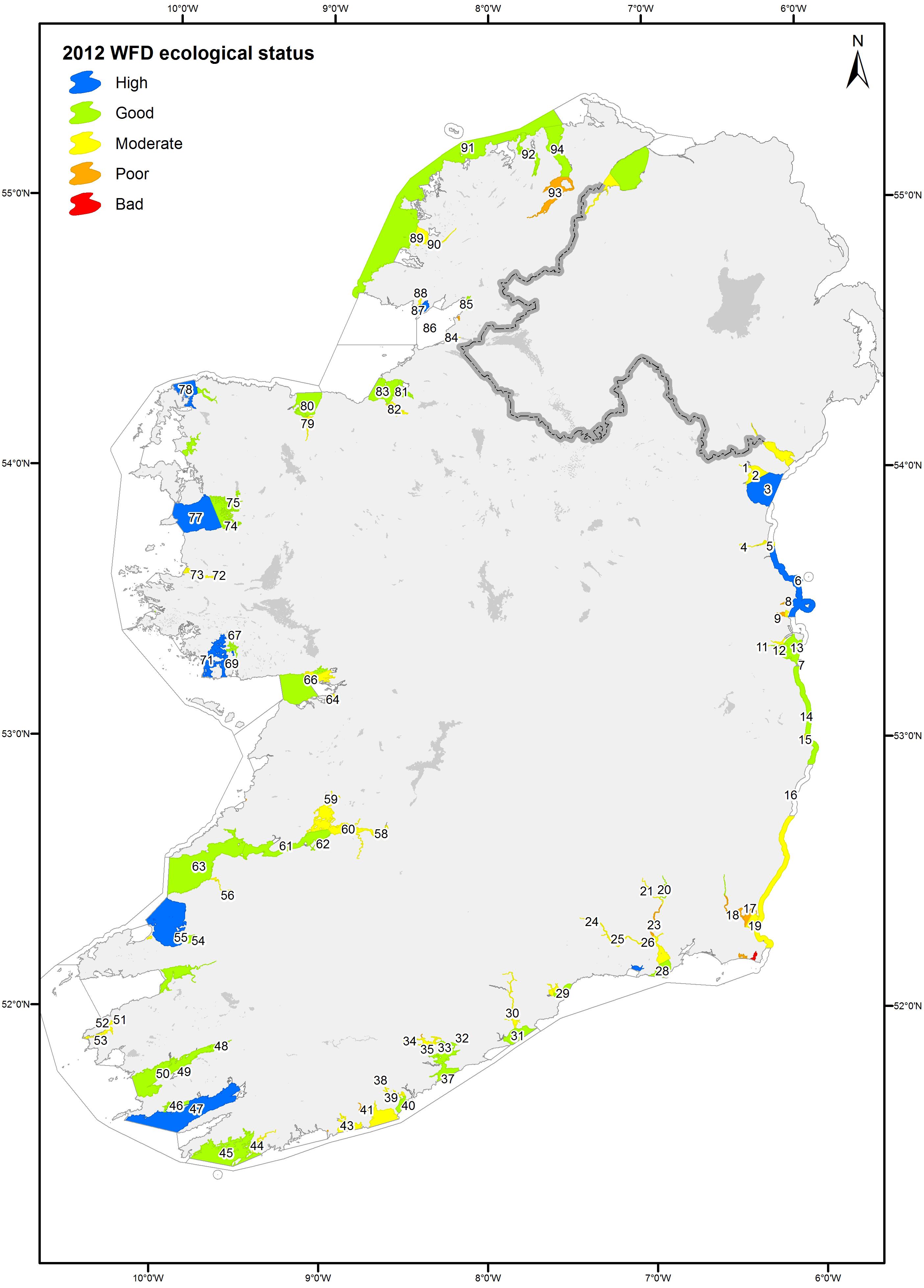
Figure 1. Map of the WFD status of monitored Irish waterbodies (2007–2012). 1, Castletown Estuary; 2, Dundalk Bay Inner; 3, Dundalk Bay Outer; 4, Boyne Estuary; 5, Boyne Estuary Plume Zone; 7, Irish Sea Dublin; 6, Northwestern Irish Sea; 8, Rogerstown Estuary; 9, Broadmeadow Water; 10, Malahide Bay; 11, Liffey Estuary Upper; 12, Liffey Estuary Lower; 13, Dublin Bay; 14, Southwestern Irish Sea Killiney Bay; 15, Broad Lough; 16, Avoca Estuary; 17, North Slob Channels; 18, Slaney Estuary Lower; 19, Wexford Harbour; 20, Upper Barrow Estuary; 21, Nore Estuary; 22, Barrow Nore Estuary Upper; 23, New Ross Port; 24, Upper Suir Estuary; 25, Middle Suir Estuary; 26, Lower Suir Estuary; 27, Barrow Suir Nore Estuary; 28, Waterford Harbour; 29, Dungarvan Harbour; 30, Blackwater Estuary Lower; 31, Youghal Bay; 32, Owenacurra Estuary; 33, North Channel; 34, Lee Estuary Lower; 35, Lough Mahon; 36, Cork Harbour; 37, Cork Harbour Outer; 38, Bandon Estuary Upper; 39, Bandon Estuary Lower; 40, Kinsale Harbour; 41, Argideen Estuary; 42, Clonakilty Harbour; 43, Clonakilty Bay; 44, Ilen Estuary; 45, Roaring Water Bay; 46, Berehaven; 47, Bantry Bay; 48, Inner Kenmare River; 49, Kilmakilloge Harbour; 50, Outer Kenmare River; 51, Cahersiveen Estuary; 52, Valentia Harbour; 53, Portmagee Channel; 54, Tralee Lee Estuary; 55, Tralee Bay Inner; 56, Feale Estuary Upper; 57, Cashen; 58, Limerick Dock; 59, Fergus Estuary; 60, Upper Shannon Estuary; 61, Lower Shannon Estuary; 62, Deel Estuary; 63, Mouth of Shannon (Has 23;27); 64, Kinvara Bay; 65, Corrib Estuary; 66, Galway Bay North Inner; 67, Loch an tSaile; 68, Loch an aibhinn; 69, Loch Tanai; 70, Camus Bay; 71, Kilkieran Bay; 72, Erriff Estuary; 73, Killary Harbour; 74, Westport Bay; 75, Newport Bay; 76, Clew Bay Inner; 77, Clew Bay; 78, Broadhaven Bay; 79, Moy Estuary; 80, Killala Bay; 81, Garavogue Estuary; 82, Ballysadare Estuary; 83, Sligo Bay; 84, Erne Estuary; 85, Donegal Bay Inner; 86, Donegal Bay; 87, McSwines Bay; 88, Killybegs Harbour; 89, Gweebarra Bay; 90, Gweebarra Estuary; 91, Northwestern Atlantic Seaboard (HAs 37;38); 92, Mulroy Bay Broadwater; 93, Swilly Estuary; 94, Lough Swilly contains information © Ordnance Survey Ireland. All rights reserved. Licence Number EN 0059208.

Monitoring stations in each waterbody are, in general, sampled three times during the months of May–September and once in the winter (January or February). Hence the sampling excludes naturally occurring spring and autumn blooms. This allows for a focus on the summer period when any growth exceedances would relate to excess nutrients entering the system. Surface and bottom water samples were collected for dissolved inorganic nitrogen (DIN) as nitrate, nitrite, and ammonia (NH4); molybdate reactive phosphorus (MRP); silicic acid (Si); and chlorophyll at each station. Nutrients were analyzed according to the Standard Methods for the Examination of Water and Waste Water². Pigments were extracted using hot methanol (not corrected for the presence of pheopigments) and was measured using a spectrophotometer (Standing Committee of Analysts, 1980). A Hydrolab DS5X Multiparameter Data Sonde was used to measure salinity, pH, dissolved oxygen, and temperature in depth profiles at each station. Transparency was estimated using a Secchi disk and used to calculate the light attenuation coefficient (Kd) and photic depth (Zp) as follows:

To determine if there was sufficient light available for phytoplankton growth the ratio of mixing depth (Zm) to photic depth (Zp) was calculated as Zm:Zp. Light limitation occurs when this ratio is greater than 5 or the eutrophic depth is <20% of the mixing depth (Cole and Cloern, 1984; Cloern, 1987). Specific details pertaining to sampling methodologies and calculations can be found in O’Boyle et al. (2015) and Ní Longphuirt et al. (2016).

To record phytoplankton abundance and community structure, the surface and bottom water samples taken for nutrients and chlorophyll were subsampled at each monitoring station. These individual samples were then mixed to give a whole waterbody sample. A subsample of the whole waterbody sample was taken in a 30-ml universal tube and preserved with Lugol’s iodine. Cell counts were undertaken in 1 ml of sample on a Sedgewick Rafter Cell using a compound microscope. Cells were recorded to an appropriate taxonomic level and damaged cells were not counted as part of the analysis. The Sedgewick Rafter Cell has a limit of detection of 1,000 cells/l. It has been proven to provide accurate results between 10,000 (ICES 2006) and 100,000 cells/l (McAlice, 1971).

Phytoplankton Index Development

The current Irish method for WFD assessment of estuarine and coastal waters is the EPA blooming tool. This tool has been inter-calibrated with other tools developed by North East Atlantic countries (Carletti and Heiskanen, 2009). The tool contains a two-stage process consisting of the determination of phytoplankton bloom frequency and biomass. In the new phytoplankton index, these two metrics were combined with the metrics developed here for abundance and community structure. The relationship between the log-transformed individual metrics and pressures was determined using Spearman’s rank coefficient (R platform). Once a relationship with pressures was established reference and class boundaries as per the WFD (high–good, good–moderate, moderate–poor, and poor–bad) for each of the metrics were identified.

Bloom Frequency

Bloom frequency was determined over the 6-year WFD cycle (four sampling occasions per year) through the analysis of taxonomic abundance of the dominant taxa (EPA, 2011). A bloom is considered to occur when the frequency of individual taxon exceeds 500,000 cells/l, at salinities of ≤17, or 250,000 cells/L for coastal waters of salinities above 17. Reference conditions are met if blooms are under a threshold of 2 for every 3 years and a high status is applied. A bloom every 2 years will place the waterbody at good status, while a bloom every year (or for 25% of sampled dates) will place the waterbody at moderate status. Ecological quality ratios (EQRs) were then calculated by dividing the reference values by the observed values.

Biomass

The median and 90th percentile chlorophyll concentrations were determined for each waterbody over a 6-year period (2007–2012). The reference conditions and class boundaries are salinity dependent; for example, the reference conditions for fully saline waters are 3.33 mg l^-1 (Carletti and Heiskanen, 2009). This gives an EQR of 1 for any concentrations at or below this value (EPA, 2006). As class boundaries had already been developed for chlorophyll in the EPA blooming tool, these were carried over to the new phytoplankton index.

Abundance

Abundance can be considered a proxy for ecological disturbance as phytoplankton community growth is directly correlated with nutrient inputs to a system. A five-point scale was developed for abundance based on the full phytoplankton dataset available for Irish estuarine waters (Table 1). The median values for all estuaries that never exhibited a bloom and were also classed as “unpolluted” (no exceedances in nutrients or oxygen levels over a 6-year period) were considered reference sites (Government of Ireland, 2009).

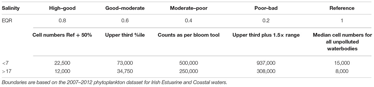
Table 1. Reference and class boundaries developed for the abundance of dominant taxa at salinities above and below 17.

The high–good boundary value was set as the reference value plus 50% of the reference value. The upper third quartile was considered the good–moderate boundary for estuaries with a salinity of more than 17, while the moderate–poor boundary was the boundary for bloom conditions (see above), as determined by the EPA blooming tool. The poor–bad boundary was the upper third quartile of all national datasets plus 1.5-times the interquartile range value [outliers were determined by the method developed by Tukey (1977) and used by Spatharis and Tsirtsis (2010)].

Community Structure

To identify structural changes in the phytoplankton community several ecological indices, which determine species richness, diversity, and evenness, were calculated for the dataset (2007–2012). These types of quantitative indices are favorable as they allow structural information about the community to be expressed as a single number (Tsirtsis and Karydis, 1998). Equations for the indices can be found in Spatharis and Tsirtsis (2010). The results of these calculations were then separated based on salinity (i.e., above and below 17 salinity). After standardization the community indices tested were compared with the abundance of the dominant taxa to determine their monotonicity (consistent increase or decrease) with this metric (Table 2). Community evenness and diversity were negatively correlated to abundance, as cell numbers increase and dominant species prevail (Spatharis and Tsirtsis, 2010). The E2 index was the evenness index with the highest correlation with the log of abundance. Similarly, Menhinick’s Index (MI) was used to represent species richness due to its strong correlation with the log of abundance (Spatharis and Tsirtsis, 2010; Ninčevič-Gladan et al., 2015). These two metrics complement each other as MI indicates the richness of the community, while the relative abundance of each species is considered with the evenness index. Hence, the two metrics combined were considered representative of community structure and were given a 0.5 weighting each for the multi-metric phytoplankton index. Because E2 and MI showed a relationship with the log abundance, the boundaries for these indices were calculated from the limits of the five-point scale developed for abundance using the equations in Table 1.

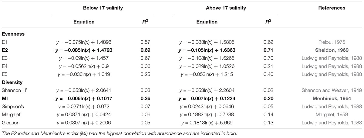
Table 2. Log regression analysis of the relationship between diversity and evenness indices and abundance of the dominant taxon.

Finally, for each metric, boundary conditions were converted into a normalized EQR by first converting the data to a numerical scale between 0 and 1, where boundaries were not equidistant. These values were then transformed into an equal-width class scale between 0 and 1, where 1 is considered high (or reference) and zero is considered low (or poor) (Table 1).

The EQR values of the four date-specific metrics (abundance, chlorophyll, E2, MDI) were calculated for the waterbodies sampled (Figure 2). While the bloom frequency was calculated over 6 years, the new multi-metric phytoplankton index was calculated from the chlorophyll, bloom frequency, abundance, and combined evenness and diversity metrics. All five metrics can be used in the calculations if an EQR for a 6-year WFD period is required (Figure 2):

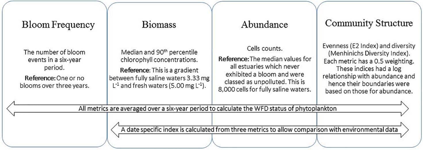
Figure 2. Schematic of the methods for calculating the multi-metric phytoplankton index over a 6-year period to comply with WFD reporting and when date and waterbody specific data are required. The lower panel shows the current phytoplankton index EQR of waterbodies grouped by their original classification as per the EPA blooming tool. For example, the waterbodies in the blue bar were all considered of “high” status but some are now of “good” status.

Only four metrics are used if only single waterbody and date-specific points are being considered (Figure 2):

Calibration of the Phytoplankton Index With the Current EPA Blooming Tool

To test the validity of the phytoplankton index the results were compared with the five assessment classes of the currently used EPA blooming tool (metrics: bloom frequency and chlorophyll) over the 2007–2012 period. The assessment classes produced were also compared with the overall WFD ecological status identified for each waterbody. The determination of overall WFD classification is a one-out-all-out system which includes data on various biological quality elements [i.e., phytoplankton, opportunistic macroalgae, macroalgal species richness, angiosperms (seagrass), benthic invertebrates, and fish], supporting quality elements including general physicochemical parameters (nutrients, biological oxygen demand, dissolved oxygen, temperature, salinity), and specific pollutants (EC, 2018). Finally, hydro-morphological risk is considered [see Government of Ireland (2009) for details of quality standards).

Statistical Analysis of Driver–Response Relationships for the Phytoplankton Index

The response of the phytoplankton index to drivers was tested using statistical analyses techniques on the R statistical software platform (R Core Team, 2013). Following the guidelines of Feld et al. (2016) the dataset was checked for outliers and square root transformed before analyses was undertaken. Pairwise Pearson correlation coefficients for all variables were undertaken to assess co-linearity (package HMisc, Harrell, 2018). Subsequently, non-linear relationships were accounted for using the variance inflation factor (package usdm, Naimi, 2015). Once collinear varibales, as determined by Pearson correlation coefficients, were removed the relationship between physicochemical parameters [salinity, residence time, Zm:Zp, temperature, MRP, DIN (summer and winter) and N:P, TON:NH4, and Si] and the phytoplankton index was examined using random forest (RF) analysis (Elith et al., 2008). Winter nutrients were added as variables as they can be considered the nutrient concentration before biological uptake during the growth period; hence, they are a proxy for loadings which were unavailable (Desmit et al., 2015). This non-parametric regression method fits several models to bootstrapped data subsets, allowing the results to be tested against the observations not used in the models. The data were then split based on predictor thresholds (Breiman, 2001). Interactions among the explanatory variables were then obtained by ranking the deviance explained by individual predictors in R using gbm.interactions. Generalized linear models were then applied to the highest ranking variables. Selection of the best model, which incorporated the least descriptor variables to fit the data, was undertaken by comparing Akaike Information Criterion (AIC) (Burnham and Anderson, 2002). Model fitness was then tested using the ANOVA function in R.

Results

Development and Testing of the Phytoplankton Index

The statistical analysis indicated significant correlations between the metrics chosen for the phytoplankton index and forcing parameters (Table 3). DIN, TON:NH4, MRP, and Si concentration gradients were strongly linked to abundance, MI, and chlorophyll. NH4 concentrations appeared to be strongly correlated to all metrics except abundance. Light conditions were linked to E2 suggesting the importance of light on the community dynamic. Residence time was also a factor which correlated strongly with abundance and chlorophyll. The analysis indicated that the metrics themselves were all correlated with each other; the correlation between E2 and abundance being the highest (Table 3).

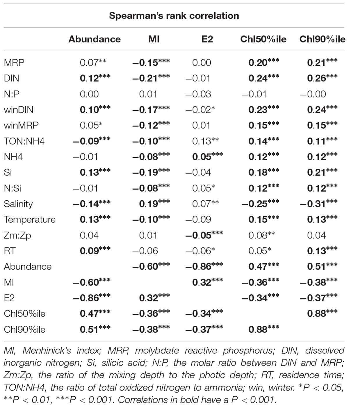
Table 3. Spearman’s rank correlation matric for the metrics chosen for the phytoplankton index (n = 1756).

The newly proposed phytoplankton index classified the status of Irish transitional and coastal waters based on the five-point WFD classification scheme. The phytoplankton index identified 28 waterbodies with “high” status, 45 waterbodies with “good” status, 14 “moderate,” and 7 “poor” waterbodies. When comparing both status and individual EQRs the new phytoplankton index performed well against the current EPA blooming tool used to determine the ecological status of phytoplankton for the WFD (Figures 3, 4). The two tools showed a linear correlation (R² = 0.85), while the newly developed phytoplankton index tended to give lower EQR values, particularly for the high-status waterbodies (Figure 4). Considering the status of the 94 waterbodies analyzed with the new phytoplankton index, 45 had the same status assignment, 48 had a lower status, and 1 had a higher status (North Slobs: poor to moderate) than the original EPA Blooming Tool.

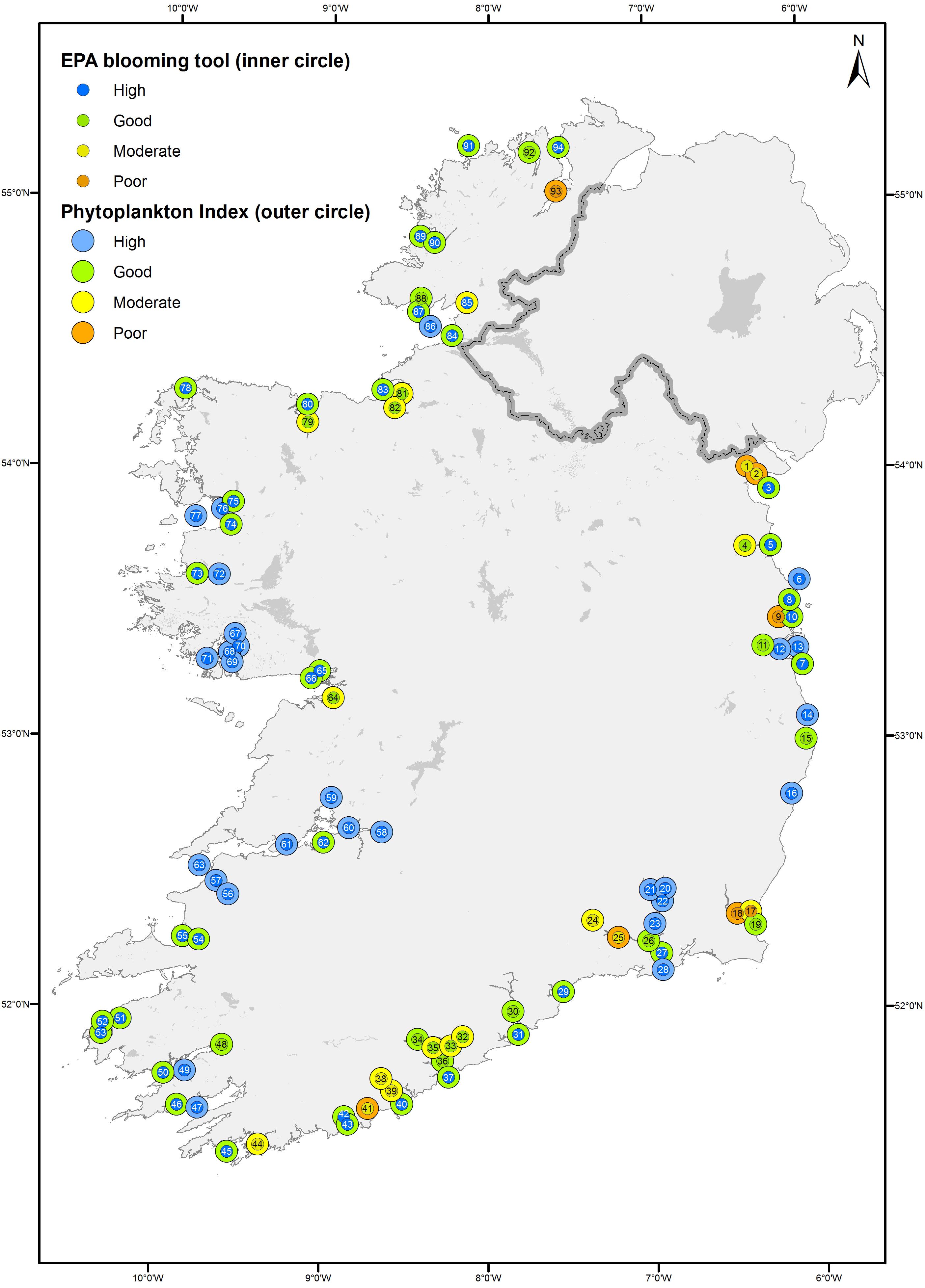
Figure 3. Map of the current status of the phytoplankton using the current EPA blooming tool (inner circles) and the newly developed phytoplankton index (outer circles) between 2007 and 2012. The index of waterbodies can be found in Figure 1 contains information © Ordnance Survey Ireland. All rights reserved. Licence Number EN 0059208.

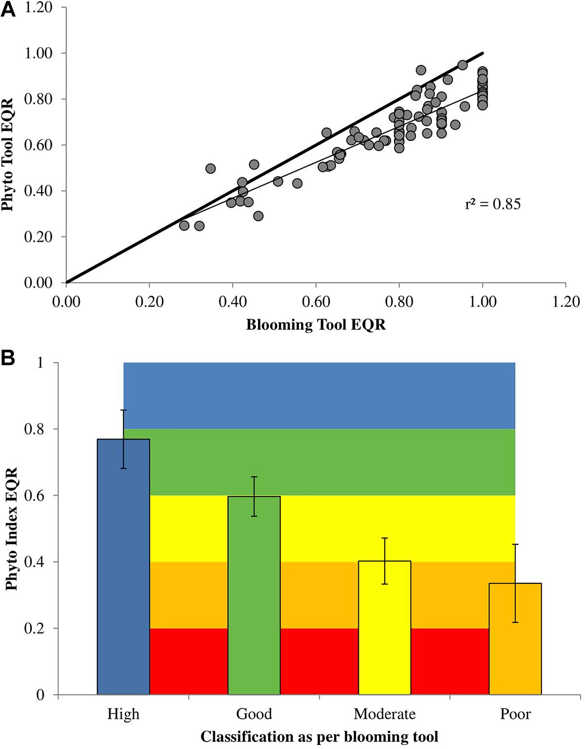
Figure 4. Comparison of the currently used EPA blooming tool against the newly developed phytoplankton index. (A) The top panel represents the new classification (phytoplankton index) grouped as per the previous classification (2007–2012). (B) The bottom panel shows a linear regression (thin line) of the phytoplankton index against the EPA blooming tool (N = 94, r² = 0.85). The thick line represents a one-to-one regression.

The new waterbody status was then compared with the overall WFD classification for the 2007–2012 period to determine if the new phytoplankton index would hypothetically alter the overall status of any of the waterbodies. The WFD status determination is a “one out all out” system; hence, the metric with the lowest classification will determine the overall status. The new phytoplankton index agreed with the overall WFD status in 39 cases, this improves upon the old tool which agreed with the WFD classification in only 25 cases. This suggests that the phytoplankton index agrees in more cases with the lowest biological or chemical metric in more waterbodies. In 45 waterbodies the new phytoplankton index designated a status that was higher than the overall status. Hence in waterbodies where the status was higher or equal to the current WFD status (84) the new phytoplankton index would not have altered the overall WFD classification for the 2007–2012 period.

In 10 cases the new phytoplankton index calculated a lower status for phytoplankton than the overall WFD status currently assigned (Table 4). This would indicate that if the new phytoplankton index was adopted these waterbodies would yield a lower status. An examination of the results from these systems showed different scenarios for coastal and transitional waterbodies. Five coastal systems (Broadhaven Bay, Valentia Harbour, Dundalk Bay Outer, McSwines Bay, and Donegal Bay Inner) were all classified as “high” for phytoplankton by the currently used EPA blooming tool and showed little or no disturbance to metrics for nutrients, oxygen, and other biological elements, while chlorophyll and phytoplankton counts and were, in general, low. However, in these systems, overall abundance and, more so, evenness and/or diversity, evidenced much lower EQR values. These lower EQRs resulted in the ecosystem classifications shifting from “high” to “good” in four systems and “high” to “moderate” in one system.

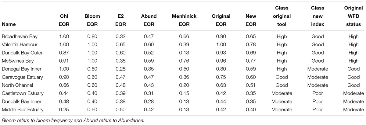
Table 4. Irish transitional and coastal waterbodies with a lower overall WFD status when the new phytoplankton index is applied.

In four transitional waterbodies (Garavogue Estuary, North Channel, Dundalk Bay Inner, and Castletown Estuary) slight to moderate disturbances were registered by the original EPA blooming tool with waterbodies being classed as either “good” or “moderate.” In these estuaries, the addition of the community structure metrics resulted in all systems dropping one classification on the scale. Although chlorophyll and/or bloom frequency EQRs did show disturbances much lower EQRs were evident for the community structure metrics. For example, in the Garavogue Estuary out of a total of 48 sampling points, 27 showed a difference between chlorophyll and abundance EQRs of over 0.4; with similar differences being observed between the chlorophyll EQR and diversity and evenness EQRs. Chaetoceros spp. (Hyalochaete), Cryptophyte spp., and Skeletonema spp. were the most prevalent species in this system and when dominant showed differences between the metrics of 0.78 ± 0.17, 0.49 ± 0.18, and 0.66 ± 0.39, respectively.

In three of these systems (North Channel, Dundalk Bay Inner, and Castletown Estuary) the original EQR was close to the boundary and so the additional metrics, while only dropping the EQR by a small amount, lead to a change of classification (Table 4). One system, the Middle Suir, showed a low chlorophyll EQR (0.25) but the bloom frequency EQR was higher (0.6), overall this resulted in a moderate status. The community structure metrics reinforced the chlorophyll EQR and resulted in a change in classification from “moderate” to “poor.” This system is dominated by Coscinodiscus spp. that have large numbers of small chloroplasts (Hasle and Syvertsen, 1997) leading to higher chlorophyll concentrations relative to cell numbers.

Overall these results indicate that disturbances to the community were not always being picked up by the chlorophyll concentration and bloom frequency. Differences between EQRs for chlorophyll and abundance in most of the 10 systems (excluding the Middle Suir Estuary) highlight how high cell abundances may not always be reflected by the chlorophyll concentration measured.

Bloom Formation

The dataset was examined to identify which species were responsible for bloom formation, and concurrently, the consistency between the chlorophyll and abundance EQRs when the phytoplankton community was in bloom (Figure 5). A bloom was considered as a cell count of the dominant species of over 500,000 cells in salinities below 17 and over 250,000 in salinities above 17. There were 612 blooms recorded in the summers between 2007 and 2016 with over 56% dominated by five species; Chaetoceros spp. (Hyalochaete) (20%), Asterionellopsis glacialis (14%), Skeletonema spp. (11%), Cryptophyte spp. (6%), and Cylindrotheca closterium (6%). These five species also dominated in periods when blooms were not recorded. In cases where the bloom was dominated by Pseudo-nitzschia > 5μm (mostly Pseudo-nitzschia delicatissima), Navicula < 10μm, Rhizosolenia setigera, Akashiwo sanguinea, and Karenia spp. (mostly Karenia mikimotoi), differences between the two metrics were consistently over 0.6. In 15 of the bloom forming species, including the dominant Chaetoceros spp. (Hyalochaete), Skeletonema spp., Cryptophyte spp., and A. glacialis, the difference between the abundance EQR and chlorophyll EQR was almost always above 0.4 (Figure 5), suggesting that at these times the chlorophyll values did not reflect the abundances present.

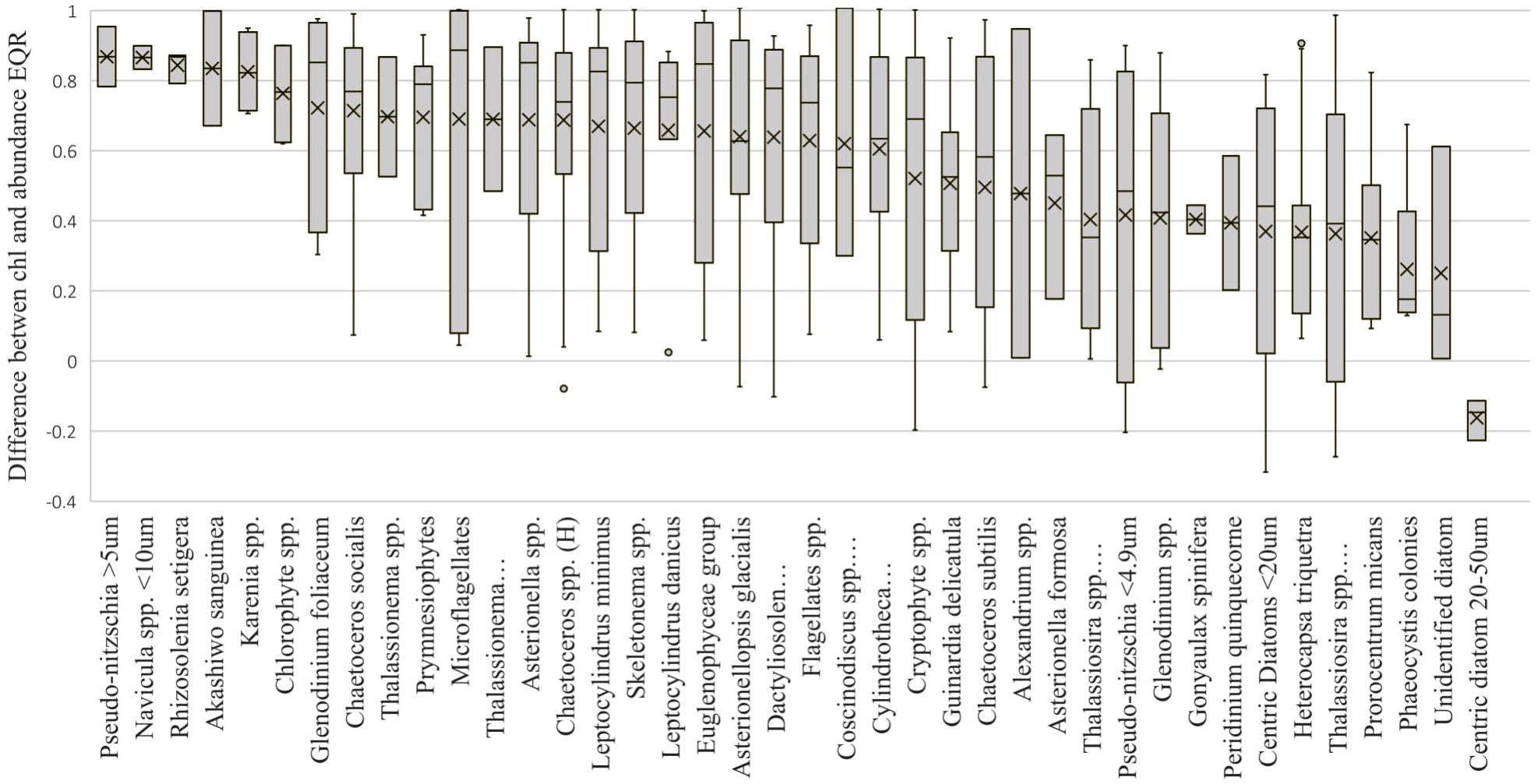
Figure 5. Boxplot representing the difference between the chlorophyll EQR and the abundance EQR relative to the species with the largest cell number during a bloom. In salinities below 17, this is a cell number of greater than 500,000 cells. In salinities above 17, this is a cell number of greater than 250,000. H refers to Hyalochaete.

Pressure–Response Relationships

Four distinctive tests were carried out using R-based statistical analysis to determine firstly, the influence of environmental drivers on the phytoplankton index of the entire dataset and during bloom periods, and secondly, the influence of drivers on the difference between chlorophyll and abundance EQRs for the entire dataset and during bloom periods. Following tests for collinearity (Pearson’s rank coefficients followed by variance inflation factors) and interactions between drivers (RF) a reduced number of parameters were chosen to build generalized linear models (GLMs). Following this AIC identified the best model for each relationship. The final model fit for each relationship identified varying parameters which influenced the results (Tables 5, 6). Hypotheses testing using ANOVAs in R suggested that all models were fit for purpose to a significance of P < 0.001.

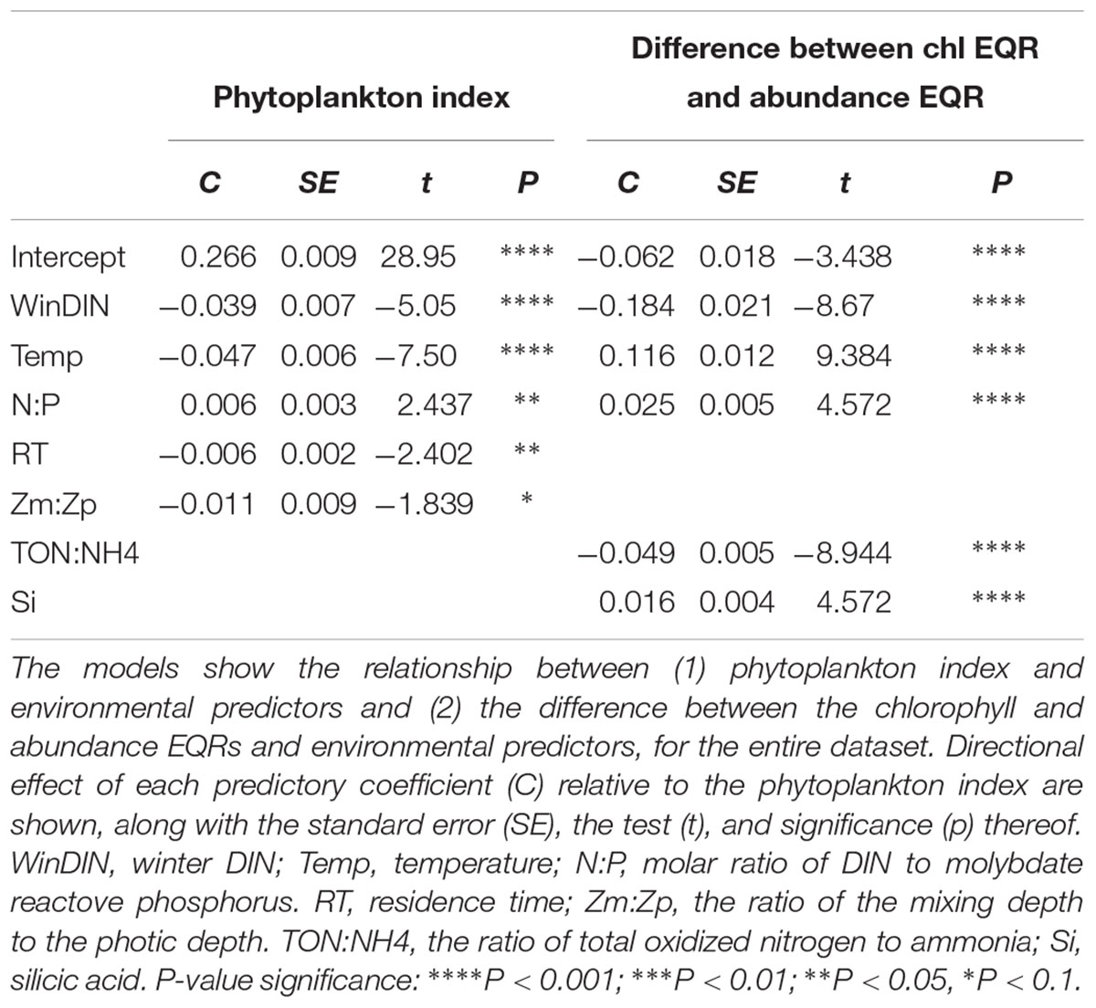
Table 5. Results of generalized linear models produced from Irish transitional and coastal water data from 2007 to 2016.

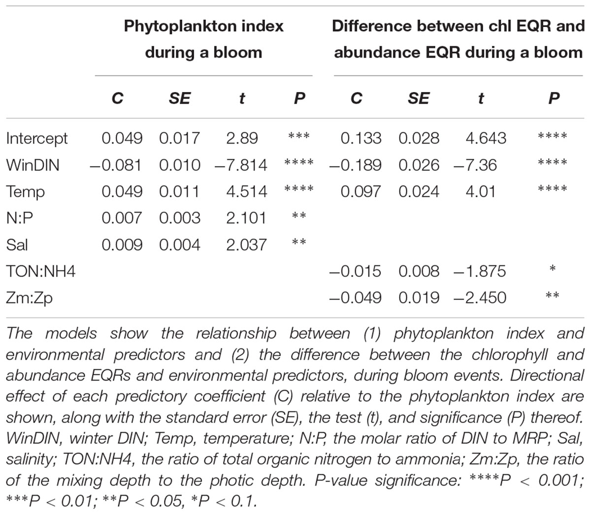
Table 6. Results of generalized linear models produced from Irish transitional and coastal water data from 2007 to 2012.

The model results indicated that for the entire dataset the phytoplankton index was negatively influenced by temperature, winter DIN, and to a lesser extent by residence time and light availability (Zm:Zp). As these parameters increased the phytoplankton index decreased (Table 5). Increased N:P had a positive impact on the phytoplankton index.

Winter DIN concentrations and the TON:NH4 ratio negatively influenced the difference between the chlorophyll and abundance EQRs (Table 5). Hence, in waterbodies where these parameters were elevated the difference between the phytoplankton index metrics tended to be reduced. Concurrently, temperature, N:P, and Si were all higher as the disparity between the two metrics increased.

During bloom events, higher concentration of winter DIN negatively impacted the entire community structure, while temperature had a positive influence (Table 6). High N:P ratios and salinity were also positively correlated to the phytoplankton index during a bloom, albeit with a weaker significance. The discrepancy between chlorophyll and abundance EQRs during a bloom appeared to be negatively influenced by winter DIN, and to a lesser extent TON:NH4 ratios and light conditions. Increased light limitation (determined by Zm:Zp) reduced the difference between the metrics. Temperature positively impacted on the difference between the metrics, so higher temperatures resulted in greater differences (Table 6).

Discussion

Phytoplankton Index Development

The multi-metric index developed in this study was proposed to provide an assessment of phytoplankton health in transitional and near coastal water systems and, further, investigate the influence of physico-chemical parameters on the phytoplankton community. The Phytoplankton index incorporates chlorophyll concentrations and bloom frequency to allow comparisons with past evaluations and in addition proposed metrics for abundance, diversity, and evenness of the community. The correlation between nutrient pressure and the individual metrics in the index validates their inclusion in the phytoplankton index developed. Correlation between the metrics themselves is also observed, and expected. As abundance and chlorophyll rise, and the number of species drops dramatically, impacting on both on species richness and the evenness of the community (Tsirtsis and Karydis, 1998; Bužančić et al., 2016).

The results indicated that the inclusion of additional metrics for community structure led to a greater level of agreement between the phytoplankton status and overall WFD status assignment between 2007 and 2012. Increasing the number of metrics in a tool is considered more robust, while allowing more sensitivity to changes in the structure of the community (Garmendia et al., 2013). At the same time, quantifying different metrics of a community can help overcome the wide diversity of cells sizes and biochemical compositions which are found in the different taxonomical groups that can comprise a phytoplankton community (Litchman and Klausmeier, 2008). In several waterbodies the inclusion of the additional metrics resulted in a reduction in the EQR and in some cases a lower status assignment for phytoplankton. This lead to greater agreement with the other biological and chemical indicators that are used to determine waterbody status under the WFD and respond to nutrient enrichment, hence reflecting an overall disturbance to the ecosystem.

Lower EQRs for one or all the metrics for abundance, diversity, and evenness suggested structural imbalances in the phytoplankton community. In some coastal systems, this structural imbalance was not reflected in the overall chlorophyll concentrations or the number of blooms recorded (Figures 3, 4 and Table 4). These waterbodies have low nutrient concentrations and anthropogenic influences are considered low (EPA, unpublished data; Ní Longphuirt et al., 2016). As such they are classed as high or good status under the WFD, but would drop a status class if the new phytoplankton index was applied. The reason for the disparity may come from either (1) extremely low phytoplankton numbers or (2) the suitability of the analyses techniques. Diversity can increase to intermediate productivity and subsequently decrease at higher cell numbers. Hence, when phytoplankton are in very low numbers diversity and evenness EQRs will be low. The data in this study were obtained from a monitoring data which, at its conception, were aimed at recording bloom events and not overall community structure. The assessment procedure uses a Sedgewick Rafter Cell, which only contains 1 ml of a sample. This may be an insufficient volume for lower productivity systems. Future applications in coastal systems will require investigation of the different counting techniques to assess the most suitable method for use with the phytoplankton index.

In several systems, the inclusion of additional metrics resulted in a reduction of the overall EQR and associated status. These results evidenced the disparity between the metrics used to determine the phytoplankton index, specifically abundance and chlorophyll. As the phytoplankton respond to increasing resource availability the community structure will comprise cells of a variety of sizes and biovolumes, with larger cells contributing most (Cloern, 2018). It has been shown that (1) larger microplankton dominate during bloom periods in estuarine systems, (2) the biovolume of these larger cells is highly variable, and (3) that biovolume will increase during a bloom as larger cells accumulate (Irwin et al., 2006; Cloern, 2018). This could explain the variability in the metrics and further the variability in EQR differences during bloom events for each species. Additional information on cell size or biovolume along with cell number would be an important consideration for phytoplankton functional traits and their contribution to the community structure (Acevedo-Trejos et al., 2015).

In Irish estuarine and near coastal systems, diatoms were the taxonomic group that dominated the bloom events, which is similar in other temperate areas (Carstensen et al., 2015). Diatoms are well adapted to varying physical and chemical gradients present in near shore estuarine and coastal systems (Lomas and Glibert, 2000) and are considered of high food value for consumers (Winder et al., 2017).

Cryptophytes also played a role representing over 6% of all blooms, slightly higher than in other temperate areas (Carstensen et al., 2015). While the biovolumes of the dominant species in this study were not measured, a comparative study in the Bay of Brest indicated that Chaetoceros spp. (Hyalochaete), Skeletonema spp., and Cryptophyte spp. have on average biovolumes of 1540, 331, and 265 μm³ cell^-1, respectively (Klein et al., unpublished in pers comm review). The biovolume of C. closterium (Lower Slaney Estuary) and A. glacialis (Ballysadare Estuary) has been measured at 325 and 444 μm³ cell^-1, respectively. In comparison Coscinodiscus spp., which often dominant in the Suir estuarine system, are considered to have high biovolumes (ca. 8,586–1,077,020 μm³ cell^-1) (Olenina et al., 2006). The relatively large size of these cells could explain the reversed relationship between the chlorophyll EQR and the lower abundance and bloom EQRs (Table 4) in this system.

While a disparity between the different metrics contained in the phytoplankton index is apparent, and in some cases, sizable, their inclusion allows the phytoplankton index to consider multiple facets of the phytoplankton community structure and consolidate them into a single EQR. Furthermore, shifts in the relationship between the different metrics can allow for trait-based diagnostics of the community. For example, a higher chlorophyll EQR relative to the abundance EQR could indicate a shift toward smaller faster growing phytoplankton in a system. This can then be correlated with other biological and physico-chemical elements of the ecosystem to understand response trajectories to climatic, physical, and anthropogenic forcings.

Phytoplankton Index Relationship With Environmental Factors

Pressure–impact relationships, a pre-requisite for ecologically meaningful indicators (Birk et al., 2012), were calculated at date and waterbody steps allowing an increased understanding of the relationship between anthropogenic pressures and physical constraints on Irish estuarine and coastal systems. The statistical analyses of the datasets indicated that the phytoplankton index responded significantly to several environmental pressures. Winter DIN, in this case considered a proxy for loadings of N to each system, had a negative relationship with the phytoplankton index over the entire dataset and concurrently when bloom events were considered alone. These results show a clear pressure–response relationship and validate the ability of a phytoplankton index, which considers not only enhanced biomass but also community structure, to respond to enrichment pressures. Concurrently, in periods where higher winter DIN concentrations were recorded the difference between the EQRs for abundance and chlorophyll was lower, indicating that the metrics were in greater agreement. As a blooming species continues to increase, its biomass peak is regulated by the nutrient supply (Chisholm, 1992), and the metrics used in the phytoplankton index will converge as both abundance and chlorophyll surpass the upper boundary levels.

The availability of lower amounts of ammonia relative to total oxidized nitrogen appeared to improve the agreement between the abundance and chlorophyll metrics, but had no influence on the overall phytoplankton index outcomes. The preference for oxidized or chemically reduced forms of N can result in shifts in biodiversity, and while diatoms appear to preferentially use nitrates, cyanobacteria, chlorophytes, and dinoflagellates may be adapted to assimilate ammonia [see Glibert (2017) for review]. While biodiversity shifts at higher relative ammonia concentrations may have occurred, the statistically significant relationship could also relate to larger overall dissolved nitrogen in the system which is mostly made up of inorganic nitrogen forms.

The GLM results suggest an increase in the ratio of nitrogen to phosphorus limits phytoplankton growth. These results reinforce the classic paradigm that reduction of a limiting nutrient (in this case phosphorus) can lead to a decrease in phytoplankton growth (Schindler et al., 2008). However, high N:P ratios are also known to alter phytoplankton biodiversity and species composition due to competition between algae with direct optimal nutrient requirements (Collos et al., 2009; Glibert and Burkholder, 2011). While not tested here, this could explain the greater differences between cell numbers and chlorophyll concentrations at higher N:P stoichiometric ratios, due to a shift in the size structure of the phytoplankton communities. The expression of this difference in metrics suggests that higher ratios will have a deleterious impact on the phytoplankton community which may not be captured using chlorophyll concentration alone.

Increased temperature was related to lower EQRs for the phytoplankton index when the entire dataset was considered. As with the nutrients, this relationship is anticipated, as growth rate, and hence the possibility of bloom occurrence, is intrinsically linked to temperature (Sherman et al., 2016). The influence of temperature on the phytoplankton community is however multifaceted; higher temperatures appeared to result in better EQRs during a bloom and at the same time correlated with greater difference between the abundance and chlorophyll EQRs in all cases. This may relate to the influence of controlling factors such as zooplankton which graze on the primary producers. At higher temperature, the grazing rate of zooplankton can accelerate faster than the growth rate of large cells, thereby curtailing their relative abundance (Nixon et al., 2009; Cloern, 2018). Small cells may thus increase in proportion in higher temperatures, augmenting their influence on the community structure. Theoretically this could result in greater divergence between the abundance and chlorophyll metrics as smaller cells will contain lower amounts of chlorophyll.

Phytoplankton biomass in Irish estuarine systems can be modulated by light and/or residence time (O’Boyle et al., 2015). The results of the current study confirm this with both physical factors impacting on the phytoplankton index. Light was also shown to impact on the difference between metrics during bloom events. As with other components limitation by light can alter the size scaling of metabolic rates, resulting in a decrease in the size-scaling exponent (Finkel et al., 2010), thus leading possible changes in phytoplankton community size structure.

The opposing predictor coefficients of the individual stressors on the phytoplankton index indicate that their interaction is, most likely, antagonistic. For example, short residence times can dampen the impact of nutrient concentrations on phytoplankton biomass (Paerl et al., 2014; Hart et al., 2015) and promote faster growing and inherently smaller phytoplankton groups (Reynolds, 2006; Hart et al., 2015). In an Irish context, O’Boyle et al. (2015) found that chlorophyll median and 90th percentile concentrations did not always correlate with nutrient concentrations due to either short residence time and/or low light conditions. The correlation of the phytoplankton index with high DIN, light, and residence time suggests that a multi-metric index may capture the complex relationship between drivers, which are not necessarily shown if biomass measurements are considered alone.

It has been recognized that a greater understanding and recognition of responses to multiple pressures are required when determining programs of measures (Carvalho et al., 2019). The expression of phytoplankton community response to modulating parameters and pressures can result in changes in the size structure, chlorophyll content, and species dominance. Metrics for chlorophyll, abundance, and community structure will represent these changes in diverse ways, while at the same time providing insight into the response mechanism. Examining the relationship between chlorophyll and abundance becomes a proxy for identifying the response of the phytoplankton community to pressures such as light conditions and ratios of available nutrients. This in turn could help flag potential issues before a more comprehensive analysis of community structure is undertaken.

Conclusion

Assessment tools which encompass both the structure and quantitative biomass response of phytoplankton communities are required to comply with the EU WFD and support management policies. The phytoplankton index proposed in this study appears to correlate well with existing methods and hence allows continuity and comparability with historic status classifications while concurrently improving the level of agreement between the status of Irish waterbodies and the overall WFD classification. Any future application of the phytoplankton index will need to consider the analytical methods used as the results appear to be influenced by the counting methods which may alter the assessment in low pressure species poor areas. The disparity between metrics shows their ability to represent different facets of the phytoplankton community structure and, in their amalgamation, a more holistic representation of the response to pressures can be portrayed.

The meta-analyses applied in this study validated the phytoplankton index through the statistically significant relationships between drivers and modulators of phytoplankton community structure and general community health. In addition, they reinforced the idea that changes in community structure, species composition, and cell size should also be considered alongside chlorophyll and abundance when considering the impact of anthropogenic forcings.

Author Contributions

SNL collated the data, undertook statistical analysis, and wrote the manuscript. GM undertook counting of phytoplankton, development of initial tool, and expert advise in phytoplankton species. RW inputted significantly to the text and provided Figures 1, 2. SO’B helped with initial tool conceptualization and reviewed the text. DS provided guidance throughout the project and reviewed the text and provided comment.

Funding

This research was fully funded under the EPA STRIVE Research Call, grant number 2012-W-FS-9. The publication fees will be provided by the EPA.

Conflict of Interest Statement

The authors declare that the research was conducted in the absence of any commercial or financial relationships that could be construed as a potential conflict of interest.

Footnotes

1. ^http://gis.epa.ie/
2. ^www.standardmethods.org

References

Acevedo-Trejos, E., Brandt, G., Bruggeman, J., and Merico, A. (2015). Mechanisms shaping size structure and functional diversity of phytoplankton communities in the ocean. Sci. Rep. 5:8918. doi: 10.1038/srep08918
Bacher, C., Duarte, P., Ferreira, J. G., Héral, M., and Raillard, O. (1998). Assessment and comparison of the Marennes-Oléron Bay (France) and Carlingford Lough (Ireland) carrying capacity with ecosystem models. Aquat. Ecol. 31, 379–394. doi: 10.1023/A:100992522830
Bharathi, M. D., Sarma, V. V. S. S., and Ramaneswari, K. (2018). Inter-annual variations in phytoplankton biomass and its composition in the tropical estuary: influence of river discharge. Mar. Poll. Bull. 129, 14–25. doi: 10.1016/j.marpolbul.2018.02.007
Birk, S., Bonne, W., Borja, A., Brucet, S., Courrat, A., Poikane, S., et al. (2012). Three hundred ways to assess Europe’s surface waters: an almost complete overview of biological methods to implement the water framework directive. Ecol. Indic. 18, 31–41.
Burnham, K. P., and Anderson, D. R. (2002). Model Selection and Multimodel Inference: A Practical Information–Theoretic Approach. 2nd Edn. Berlin: Springer.
Bužančić, M., Ninčević-Gladan,Ž, Marasović, I., Kušpilić, G., and Grbec, B. (2016). Eutrophication influence on phytoplankton composition in three bays on the eastern Adriatic coast. Oceanology 58, 302–316.
Carletti, A., and Heiskanen, A.-S. (2009). Water framework directive intercalibration technical report – part 3: coastal and transitional waters. JRC Sci. Techn. Rep. 240, 138–169.
Carlsson, P., and Granéli, E. (1999). Effects of N:P:Si ratios and zooplankton grazing on phytoplankton communities in the northern Adriatic Sea. II. Phytoplankton species composition. Aquat. Mar. Ecol. 18, 55–65. doi: 10.3354/ame018055
Carstensen, J., Klais, R., and Cloern, J. (2015). Phytoplankton blooms in estuarine and coastal waters: seasonal patterns and key species. Est. Coast. Shelf Sci. 162, 98–109. doi: 10.1016/j.ecss.2015.05.005
Carvalho, L., Mackay, E. B., Cardoso, A. C., Baattrup-Pedersen, A., Birk, S., Blackstock, K. L., et al. (2019). Protecting and restoring Europe’s waters: an analysis of the future development needs of the water framework directive. Sci. Tot. Environ. 658, 1228–1238. doi: 10.1016/j.scitotenv.2018.12.255
Chisholm, S. W. (1992). “Phytoplankton size,” in Primary Production and Biogeochemical Cycles in the Sea. eds P. G. Falkowski and A. D. Woodhead (New York, NY: Plenum Press), 213–237.
Cloern, J. E. (1987). Turbidity as a control on phytoplankton biomass and productivity in estuaries. Cont. Shelf Res. 7, 1367–1381. doi: 10.1039/b927243g
Cloern, J. E. (2018). Why large cells dominate estuarine phytoplankton limnol. Oceanography 63, 392–409. doi: 10.1002/lno.10749
Cloern, J. E., Foster, S. Q., and Kleckner, A. E. (2014). Phytoplankton primary production in the world’s estuarine-coastal ecosystems. Biogeosciences 11, 2477–2501. doi: 10.5194/bg-11-2477-2014
Cole, B. E., and Cloern, J. E. (1984). Significance of biomass and light availability to phytoplankton productivity in San Francisco Bay. Mar. Ecol. Prog. Ser. 17, 15–24.
Collos, Y., Bec, B., Jauzein, C., Abadie, E., Laugier, T., Lautier, J., et al. (2009). Oligotrophication and emergence of picocyanobacteriaand a toxic dinoflagellate in Thau Lagoon, southern France. J. Sea Res. 61, 68–75. doi: 10.1016/j.seares.2008.05.008
Desmit, X., Ruddick, K., and Lacroix, G. (2015). Salinity predicts the distribution of chlorophyll a spring peak in the southern North Sea continental waters. J. Sea Res. 103, 59–74. doi: 10.1016/j.seares.2015.02.007
Devlin, M., Barry, J., Painting, S., and Best, M. (2009). Extending the phytoplankton tool kit for the UK water framework directive: indicators of phytoplankton community structure. Hydrobiologica 633, 151–168.
Domingues, R. B., Barbosa, A. B., and Galvão, H. M. (2008). Constraints on the use of phytoplankton as a biological quality element within the water frame directive in Portuguese Waters. Mar. Poll. Bull. 56, 1389–1395. doi: 10.1016/j.marpolbul.2008.05.006
EC (2000). Directive 2000/60/EC of the European Parliament and of the Council Establishing a Framework for the Community Action in the Field of Water Policy. Brussels: European Commission.
EC (2018). COMMISSION DECISION (EU) 2018/229 of 12 February 2018 Establishing, Pursuant to Directive 2000/60/EC of the European Parliament and of the Council, the Values of the Member State Monitoring System Classifications as a Result of the Inter-Calibration Exercise and Repealing Commission Decision 2013/480/EU. Brussels: European Commission.
Elith, J., Leathwick, J. R., and Hastie, T. (2008). A working guide to boosted regression trees. J. Anim. Ecol. 77, 802–813. doi: 10.1111/j.1365-2656.2008.01390.x
EPA (2006). EU Water Framework Directive Monitoring Programme. Wexford: Environmental Protection Agency.
EPA (2011). Water Framework Directive Status Update 2007-2009. Wexford: Environmental Protection Agency.
Facca, C., Aubrey, F. B., Socal, G., Ponis, E., Acri, F., Bianchi, F., et al. (2014). Description of a multimetric phytoplankton index (MPI) for the assessment of transitional waters. Mar. Poll. Bull. 79, 145–154. doi: 10.1016/j.marpolbul.2013.12.025
Feld, C. K., Segurado, P., and Gutiérrez-Cánovas, C. (2016). Analysing the impact of multiple stressors in aquatic biomonitoring data: a ‘cookbook’ with applications in R. Sci. Tot. Environ. 573, 1320–1339. doi: 10.1016/j.scitotenv.2016.06.243
Ferreira, J. G., Vale, C., Soares, C. V., Salas, F., Stacey, P. E., Bricker, S. B., et al. (2007). Monitoring of coastal and transitional waters under the E.U. Water Framework Directive. Environ. Monit. Assess. 135, 195–216.
Finkel, Z. V., Beardall, J., Flynn, K. J., Quigg, A., Rees, T. A. V., and Raven, J. A. (2010). Phytoplankton in a changing world: cell size and elemental stoichiometry. J. Plankton Res. 32, 119–137. doi: 10.1093/plankt/fbp098
Garmendia, M., Borja,Á, Franco, J., and Revilla, M. (2013). Phytoplankton composition indicators for the assessment of eutrophication in marine waters: present state and challenges within the European directives. Mar Pol. Bull. 66, 7–16. doi: 10.1016/j.marpolbul.2012.10.005
Giordani, G., Zaldívar, J. M., and Viaroli, P. (2009). Simple tools for assessing water quality and trophic status in transitional water ecosystems. Ecol. Indicat. 9, 982–991.
Glibert, P. M. (2017). Eutrophication, harmful algae and biodiversity — challenging paradigms in a world of complex nutrient changes. Mar. Poll. Bull. 124, 591–606. doi: 10.1016/j.marpolbul.2017.04.027
Glibert, P. M., and Burkholder, J. M. (2011). Harmful algal blooms and eutrophication: strategies for nutrient uptake and growth outside the Redfield comfort zone. Chin. J. Limnol. Oceanol. 29, 724–738.
Government of Ireland (2009). S.I. No. 272/2009 – European Communities Environmental Objectives (Surface Waters) Regulations 2009. Available at: http://www.irishstatutebook.ie/eli/2009/si/272/made/en/print (accessed June 28, 2018).
Harrell, F. E. Jr. (2018). Hmisc: Harrell Miscellaneous. Available at: https://cran.rproject.org/web/packages/Hmisc/index.html (accessed June 2018).
Hart, J. A., Phlips, E. J., Badylak, S., Dix, N., Petrinec, K., Mathews, A. L., et al. (2015). Phytoplankton biomass and composition in a well-flushed, sub-tropical estuary: the contrasting effects of hydrology, nutrient loads and allochthonous influences. Mar. Environ. Res. 112, 9–20. doi: 10.1016/j.marenvres.2015.08.010
Hasle, G. R., and Syvertsen, E. E. (1997). “Marine diatoms,” in Identifying Marine Phytoplankton, ed. C. R. Tomas (San Diego, CA: Academic Press, Inc.), 5–385.
Houde, E. D., and Rutherford, E. S. (1993). Recent trends in estuarine fisheries: predictions of fish production and yield. Estuaries 16, 161–176. doi: 10.2307/1352488
Irwin, A. J., Finkel, Z. V., Schofield, O. M. E., and Falkowski, P. G. (2006). Scaling-up from nutrient physiology to the size-structure of phytoplankton communities. J. Plank. Res. 28, 459–471.
Lacouture, R. V., Johnson, J. M., Buchanan, C., and Marshall, H. G. (2006). Phytoplankton index of biotic integrity for Chesapeake Bay and its tidal tributaries. Estuar. Coasts 29, 598–616.
Litchman, E., and Klausmeier, C. A. (2008). Trait-based community ecology of phytoplankton. Annu. Rev. Ecol. Evol. Syst. 39, 615–639.
Lomas, M. W., and Glibert, P. M. (2000). Comparisons of nitrate uptake, storage and reduction in marine diatoms and flagellates. J. Phycol. 36, 903–913.
Ludwig, A. J., and Reynolds, J. F. (1988). Statistical Ecology: A Primer on Methods and Computing. New York, NY: John Wiley and Sons.
Lugoli, F., Garmendia, M., Lehtinen, S., Kauppila, P., Moncheva, S., Revilla, M., et al. (2012). Application of a new multi-metric phytoplankton index to the assessment of ecological status in marine and transitional waters. Ecol. Indicat. 23, 338–355.
McAlice, B. J. (1971). Phytoplankton sampling with the Sedgwick-rafter cell. Limnol. Oceangr. 16, 19–28. doi: 10.4319/lo.1971.16.1.0019
Menhinick, E. P. (1964). A comparison of some species-individuals’ diversity indices applied to samples of field insects. Ecology 45, 859–861. doi: 10.2307/1934933
Naimi, B. (2015). Usdm: Uncertainty Analysis for Species Distribution Models. Available at: https://cran.r-project.org/web/packages/usdm/index.html (accessed June 2018).
Ní Longphuirt, S., Mockler, E. M., O’Boyle, S., Wynne, C., and Stengel, D. B. (2016). Linking changes in nutrient source load to estuarine responses: an Irish perspective. Biol. Environ. Proc. R. Irish Acad. 116B, 295–311. doi: 10.3318/bioe.2016.21
Ninčevič-Gladan, Z., Bužančić, M., Kušpilić, G., Grbec, B., Matijević, I., and Morović, M. (2015). The response of phytoplankton community to anthropogenic pressure gradient in the coastal waters of the Adriatic Sea. Ecol. Indicat. 56, 106–115. doi: 10.1016/l.ecolind.2015.03.018
Nixon, S. W. (1995). Coastal marine eutrophication: a definition, social causes, and future concerns. Ophelia 41, 199–219. doi: 10.1080/00785236.1995.10422044
Nixon, S. W., Fulweiler, R. W., Buckley, B. A., Granger, S. L., Nowicki, B. L., and Henry, K. M. (2009). The impact of changing climate on phenology, productivity, and benthic-pelagic coupling in Narragansett Bay. Estuar. Coast. Shelf Sci. 82, 1–18. doi: 10.1016/j.ecss.2008.12.016
O’Boyle, S., Quinn, R., Dunne, N., Mockler, E., and Ní Longphuirt, S. (2016). What have we learned from over two decades of monitoring riverine nutrient inputs to Ireland’s marine environment? Biol. Environ. Proc. R. Irish Acad. 116B, 313–327. doi: 10.3318/bioe.2016.23
O’Boyle, S., Wilkes, R. J., Mcdermott, G., Ní Longphuirt, S., and Murray, C. (2015). Factors affecting the accumulation of phytoplankton biomass in Irish estuaries in nearshore coastal waters: a conceptual model. Estuar. Coast. Shelf Sci. 155, 75–88. doi: 10.1016/j.ecss.2015.01.007
Olenina, I., Hajdu, S., Edler, L., Andersson, A., Wasmund, N., Busch, S., et al. (2006). Biovolumes and size-classes of phytoplankton in the Baltic Sea HELCOM Balt.Sea. Environ. Proc. 106:144.
Paerl, H. W., Hall, N. S., Pierels, L., Rossignol, K. L., and Joyner, A. R. (2014). Hydrological variability and its control of phytoplankton community structure and function in two shallow, coastal lagoonal ecosystems: the Neuse and New River Estuaries, North Carolina, USA. Estuar. Coasts 37, 31–45. doi: 10.1007/s12237-013-9686-0
R Core Team (2013). R: A language and environment for statistical computing. Vienna: R Foundation for Statistical Computing.
Schindler, D. W., Hecky, R. E., Findlay, D. L., Stainton, M. P., Parker, B. R., Paterson, M. J., et al. (2008). Eutrophication of lakes cannot be controlled by reducing nitrogen input: results of a 37-year whole-ecosystem experiment. Proc. Natl. Acad. Sci. U.S.A. 105, 11254–11258. doi: 10.1073/pnas.0805108105
Shannon, C. E., and Weaver, W. (1949). The Mathematical Theory of Communication. Urbana: University of Illinois Press.
Sherman, E., Moore, J. K., Primeau, F., and Tanouye, D. (2016). Temperature influence on phytoplankton community growth rates. Global Biogeochem. Cycles 30, 550–559.
Smayda, T. J. (2004). “Eutrophication and phytoplankton,” in Drainage Basin Nutrient Inputs and Eutrophication: an Integrated Approach, eds P. Wassmann and K. Olli (Tromsø: University of Tromsø), 89–98.
Spatharis, S., and Tsirtsis, G. (2010). Ecological quality scales based on phytoplankton for the implementation of water framework directive in the eastern mediterranean. Ecol. Indicat. 10, 840–847.
Standing Committee of Analysts (1980). The Determination of Chlorophyll a in Aquatic Environments. London: Her Majesty’s Stationary Office.
Tett, P., Carreira, C., Mills, D. K., van Leeuwen, S., Foden, J., Bresnan, E., et al. (2008). Use of a phytoplankton community Index to assess the health of coastal waters. ICES. J. Mar. Sci. 65, 1475–1482. doi: 10.1093/icesjms/fsn161
Tsirtsis, G., and Karydis, M. (1998). Evaluation of phytoplankton community indices for detecting eutrophic trends in marine environments. Environ. Mon. Assess. 50, 255–269. doi: 10.1023/A:1005883015373
Tukey, J. W. (1977). Exploratory Data Analysis. Menlo Park, CA: Addison-Wesley Publishing Company Reading, Mass.
Keywords: bloom, water framework directive, phytoplankton, estuarine, eutrophication
Citation: Ní Longphuirt S, McDermott G, O’Boyle S, Wilkes R and Stengel DB (2019) Decoupling Abundance and Biomass of Phytoplankton Communities Under Different Environmental Controls: A New Multi-Metric Index. Front. Mar. Sci. 6:312. doi: 10.3389/fmars.2019.00312
Received: 01 October 2018; Accepted: 27 May 2019;
Published: 13 June 2019.
Edited by:
Katherine Richardson, University of Copenhagen, DenmarkReviewed by:
Erik Askov Mousing, Norwegian Institute of Marine Research (IMR), NorwayMichelle Jillian Devlin, Centre for Environment, Fisheries and Aquaculture Science (CEFAS), United Kingdom
Copyright © 2019 Ní Longphuirt, McDermott, O’Boyle, Wilkes and Stengel. This is an open-access article distributed under the terms of the Creative Commons Attribution License (CC BY). The use, distribution or reproduction in other forums is permitted, provided the original author(s) and the copyright owner(s) are credited and that the original publication in this journal is cited, in accordance with accepted academic practice. No use, distribution or reproduction is permitted which does not comply with these terms.
*Correspondence: Sorcha Ní Longphuirt, s.nilongphuirt@epa.ie