Argo Data 1999–2019: Two Million Temperature-Salinity Profiles and Subsurface Velocity Observations From a Global Array of Profiling Floats

Introduction

Prior to the turn of the 21st century, comprehensive in-situ ocean observations were difficult to obtain. Temperature and salinity data were collected mainly from ships and moored buoys, and were biased geographically toward the northern hemisphere oceans, where most of these platforms operated. Measurements acquired during ship-based surveys were mostly along transect lines, thus leaving large spatial gaps in sampling. Temporal coverage of data was also uneven, as sampling was limited to the years and seasons when ships were available. Data from the high latitudes during winter were especially sparse. Large-scale measurements of upper ocean temperature were made possible by the advent of the expendable bathythermograph (XBT), but with no accompanying salinity measurements and with relatively limited data coverage in the southern hemisphere. These limitations in spatial and temporal oceanographic data coverage, compounded by a lack of any systematic subsurface salinity data, impaired the progress in operational oceanography and ocean climate research.

In 1998, the Year of the Oceans, an international team of scientists proposed a design for a global array of autonomous profiling floats to enhance the temperature and salinity measurements of the upper ocean (Argo Science Team, 1998). This new network, called Argo, would be integrated into the global ocean observing system, filling in the large data gaps that existed in the in-situ ocean observations at that time. The initial endorsements came from the CLIVAR Upper Ocean Panel (UOP) and the Global Ocean Data Assimilation Experiment (GODAE). The Argo Science Team (later renamed the Argo Steering Team) was constituted at a joint meeting of the CLIVAR UOP and GODAE in mid-1998. The Argo Program was further endorsed as a pilot program by the Global Ocean Observing System (GOOS).

The name Argo was chosen because of the program's complementary nature with Jason, the Centre National d'Études Spatiales/National Aeronautics and Space Administration (CNES/NASA) satellite oceanography sea level mission (Roemmich and Owens, 2000). In Greek mythology, Jason sailed in a ship called Argo with his crew, the Argonauts. In oceanography, Jason and Argo together would provide regular global sea surface height and subsurface temperature and salinity measurements, the variables that are necessary for the proper interpretation of sea surface height. Argo's aim was to provide sustained and global sampling of subsurface temperature-salinity-pressure profiles and velocity fields by using the autonomous profiling float technology. Today, as an element of the GOOS, Argo has important synergies with many of the other in-situ observation networks, which include shipboard repeat hydrography, moored buoys, surface drifters, XBT, glider transects, sea level stations, and animal-borne profiling. The integration of the GOOS is coordinated by the Observations Coordination Group (OCG), with the Joint Technical Commission for Oceanography and Marine Meteorology in-situ Observations Programme Support Centre (JCOMMOPS) providing the technical support.

Conceptually, the design of the Argo array evolved from the World Ocean Circulation Experiment (WOCE)'s shipboard hydrographic program, deployment of Argo-type floats, and its XBT network. The initial design of Argo called for the deployment of over 3,000 profiling floats in a 3° × 3° array in the ice-free open ocean between 60°N and 60°S (Argo Science Team, 1998). In a departure from the practices of that era, the data from these floats would be freely disseminated in real-time, allowing use in operational ocean and atmospheric models. The data would be further quality-controlled, and this “delayed-mode” version would also be shared freely with the scientific community. It was recognized that Argo would require an international collaboration similar to that developed by WOCE. The floats would be deployed by separate groups from participating countries, but the data would be shared internationally.

The standard Argo mission is known as “park-and-profile” (Figure 1). The floats park at a target pressure of 1,000 decibars and drift with the ocean currents. Pressure in decibars (dbar; 1 dbar = 10,000 Pa) is approximately equal to depth in meters. The Argo park level of 1,000 dbar was chosen to extend the absolute velocity database collected during WOCE, which employed that level based on its favorable signal-to-noise ratio. Every 10 days the floats descend to 2,000 dbar and then collect a vertical profile of temperature and salinity during ascent to the surface. The positions of the floats at the sea surface are determined by orbiting platforms, and the data are transmitted via satellite back to shore. The floats then return to their target park pressure and the cycle is repeated. Deployments of Argo floats began in 1999, and the 3,000-float goal was reached in November 2007. Argo collected its one-millionth profile in October 2012 and its two-millionth profile in September 2018.

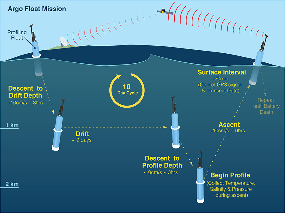
Figure 1. A schematic illustration of the standard Argo “park-and-profile” mission. The surface interval of ~20 min is applicable to floats that use Iridium satellite communication; floats that use ARGOS satellite communication require surface interval of several hours for data telemetry. [Source: Woods Hole Oceanographic Institution].

This paper describes the pressure (P), temperature (T), salinity (S), and subsurface velocity data from the Argo Program: the instrumentation used, the technical problems encountered, the scientific quality of the data, the data distribution system, and how the dataset has evolved in response to new technologies. It has been over 20 years since the first deployment of Argo floats in 1999. This has been a long journey for the scientists who first conceived the Argo array, and yet it is but a short step toward the goal of sustaining a comprehensive global ocean observation system. This paper therefore serves the dual purpose of documenting the characteristics and accuracy of the core Argo dataset from its inception to 2019, as well as foretelling the expansion of this global ocean dataset into 2020 and beyond.

Instrumentation Used in Argo

Platform History

The present-day autonomous profiling float was developed from the neutrally buoyant float with short-range acoustic tracking (Swallow, 1955; Gould, 2005). During WOCE, Russ Davis and Doug Webb in the United States, and teams at L'Institut Français de Recherche pour l'Exploitation de la Mer (Ifremer) in France, equipped a new generation of floats with a pumping system and satellite navigation, so they could cycle repeatedly to the sea surface for satellite tracking in the ice-free ocean (Davis et al., 1992; Ollitrault et al., 1994a). The float density was changed by pumping oil stored in an internal reservoir into an external bladder to ascend, and by deflating the bladder to descend. In WOCE, these early-model floats were used to determine the absolute velocity field at the park level. MARVOR floats were deployed in the eastern North Atlantic Ocean (Speer et al., 1999) and in the Brazil Basin of the South Atlantic Ocean (Ollitrault et al., 1994b). Autonomous Lagrangian Circulation Explorer (ALACE) floats were deployed more widely (e.g., Davis, 1998). By the end of the 1990s, the addition of conductivity-temperature-depth¹ (CTD) sensors allowed for the collection of vertical profiles of temperature and salinity during each ascent to the sea surface (Loaec et al., 1998; Davis et al., 2001). Early inductive-type CTDs used on floats did not perform reliably, but the first pumped electrode-type CTD, a prototype supplied by Sea-Bird Scientific (used on Float 063, with WMO ID² 41862, deployed by the University of Washington in 1997), demonstrated that an accuracy of 0.01 in Practical Salinity Scale 1978 (PSS-78) was obtainable for float salinity over the course of several years (Argo Science Team, 1998).

As Argo developed, early float models used in WOCE were augmented by newer ones. As a result, a variety of float types have been used in Argo. These include:

• the PROVOR and the ARVOR, designed by Ifremer and built by nke Instrumentation

• the APEX, built by Teledyne Webb Research

• the SOLO-I and the SOLO-II, built by³ Scripps Institution of Oceanography

• the S2A, a commercial version of SOLO-II, built by MRV Systems

• the NAVIS, built by Sea-Bird Scientific

• the NOVA, built by MetOcean

• the NINJA, built by Tsurumi-Seiki

Table 1 shows the percentage of profiles that each of these float types has obtained.

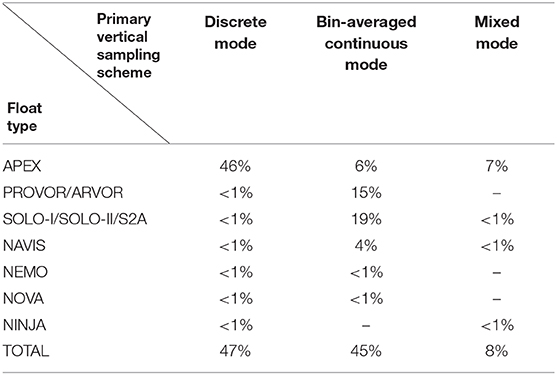
Table 1. The various float types and their primary vertical sampling schemes as a percentage of the total number of primary profiles in Argo, as of April 2019.

CTD Units and Pre-deployment Sensor Checks

The CTD units fitted to most Argo floats have been manufactured by two companies, Sea-Bird Scientific (SBE) and Falmouth Scientific (FSI). The FSI unit was an inductive-style sensor and was only used in a small number of floats (about 3% as of 2019) in the beginning of the program. The SBE CTD unit is an enclosed pump unit (Figure 2) and has been used on almost all Argo floats since 2005. The details of the operation of the SBE CTD unit are described in Riser et al. (2008) and Riser et al. (2018). Briefly, the CTD pump draws seawater through the intake past the temperature sensor and then through the conductivity cell. Fluid in the cell exits through an exhaust port that is aligned perpendicular to the intake, so as not to contaminate the water entering the cell. The pressure sensor is mounted on the float end cap, close to the CTD unit. The temperature and electrical conductivity of the seawater sample in the cell are measured directly. From temperature, pressure, and conductivity, salinity (in PSS-78) can be computed by using the equation of state for seawater (Fofonoff and Millard, 1983).

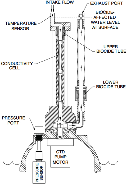
Figure 2. A schematic drawing of a Sea-Bird Scientific CTD unit. [Source: from (Riser et al., 2018). Copyright 2018 American Geophysical Union (AGU)].

Sea-Bird Scientific has supplied two main CTD models for Argo floats: the SBE-41 and the SBE-41CP. The SBE-41 operates in the spot-sampling mode only and collects discrete samples according to a pre-set pressure table, with the CTD pump turned off between samples. The SBE-41CP has the capability to operate in both the spot-sampling mode and the continuous-profiling (CP) mode. When used in the CP mode, the CTD pump remains on and samples are collected at nominally 1 Hz. These continuous data are then bin-averaged onboard the float before they are transmitted by satellite.

The manufacturer-quoted initial accuracies for the SBE-41/41CP, as of 2019, are 2 dbar for pressure⁴, 0.002°C for temperature, and 0.0035 PSS-78 for salinity. Some float-providing groups conduct independent CTD accuracy checks to ensure that the sensor calibrations are within the manufacturer's specifications before float deployment. The Euro-Argo group performs systematic tests of profiling floats in Ifremer's 20 m-depth seawater pool. Floats are tested simultaneously in batches of 10–40, and multiple test cycles (typically 6) are conducted over a 3-day period. The 20 m-depth profiles and park-phase data at pool depth are compared at sensor resolution level. As the test pool is a stable seawater environment, float sensors whose measurements differ from the ensemble averages are considered anomalous and are thus returned to the manufacturer.

At the University of Washington (UW), pre-deployment sensor checks consist of checking the pressure sensor and the conductivity cell. The pressure sensor is checked against a highly accurate Type T Hydraulic Deadweight Tester. Two sets of data are collected: the first at room temperature and the second at cold temperature, to simulate what the floats would experience in the ocean. At each of these two temperatures, measurements are collected at 5 different pressure levels spanning 0–2,000 dbar. At each pressure level, 3 consecutive measurements within 1 dbar of each other are taken and a median filter is applied to get the final value. If any of the final values from the test CTD differ from the standard pressure by more than 2.5 dbar, the test CTD is returned to the manufacturer for recalibration. The Commonwealth Scientific and Industrial Research Organization (CSIRO) at Hobart, Australia, also conducts a similar deadweight pressure test at 20,000 kPa and 20°C. For the conductivity cell check, UW uses an in-house reference SBE-41 CTD that is calibrated regularly at Sea-Bird Scientific. The reference CTD and the test CTD are then plumbed to sample from the same batch of standard seawater with the aid of a peristaltic pump. The mean values from 100+ samples are compared. If the mean values differ by <0.005 PSS-78, the test CTD is accepted for deployment. The Argo group at NOAA Pacific Marine Environmental Laboratory (PMEL) does a similar conductivity cell check.

At the Japan Agency for Marine-Earth Science and Technology (JAMSTEC), shipboard CTD casts are conducted as often as possible when floats are deployed from research vessels. By evaluating float temperature values at deployment against shipboard CTD casts over 300 floats, JAMSTEC found that the differences were mostly within ± 0.005°C.

Satellite Communications

At the beginning of Argo, almost all floats transmitted their data via the Système ARGOS⁵ location and data transmission system (Argos-2), operated by Collecte Localization Satellites (CLS/Argos in Toulouse, France, and CLS/America in Maryland, USA). These are one-way, low-bandwidth satellites, with an effective data throughput of no more than 1 bit per second. The data transmission rates are such that in order to guarantee error free data reception and location in all weather conditions, the float must spend between 6 and 18 h transmitting at the sea surface.

Other satellite transmission systems have been used on profiling floats over the history of Argo. The Argos-3 satellite system was implemented on ARVOR floats for evaluation of its interactive low- and high-data-rate modes, both offering bidirectional transmission and a higher throughput than the older Argos-2 satellite system. While the low-data-rate mode offered faster data transmissions, the high-data-rate mode suffered from electromagnetic noise around Europe (André et al., 2015). At regional scales, non-global transmission systems such as BeiDou in Asia and Orbcomm in North America have also had limited use on profiling floats.

At present, the majority of Argo floats (77% of the active fleet as of March 2020) use the Iridium satellite system for data communication (Figure 3). There are two methods by which data can be transmitted using Iridium (Riser et al., 2018). The first method uses a Circuit-Switched Data (CSD) channel and is usually routed via the Router-Based Unrestricted Digital Internetworking Connectivity Solutions (RUDICS). The second method uses Short-Burst Data (SBD) and is analogous to sending an SMS text message. In general, the CSD method is used when a large quantity of data needs to be transmitted, while the SBD method is used when the volume of data being transmitted is relatively small or when the data have been compressed.

Figure 3. Argo's geographical coverage by telecommunication type. This map shows the launch location of all floats deployed within the Argo Program, as of January 2020. The red and blue dots denote floats that used Iridium and ARGOS telecommunications, respectively. [Source: JCOMMOPS].

The first Argo float that used Iridium communication was deployed in 2005. Since then, Iridium has become the preferred means of satellite communication because it is a two-way, higher bandwidth system, with transmission rates of around 300 bits per second. Iridium allows more data to be transmitted in a shorter period of time than via Système ARGOS. The transition to Iridium dramatically reduced the time spent on the sea surface to <20 min for each cycle. Two-way communication via Iridium makes it possible to send instructions to the float for troubleshooting or for changing the float's mission (Roemmich et al., 2004). As a result of this transition from unidirectional to faster bidirectional satellite communication, there is now a large variety of float sampling missions and an even larger volume of float data. In 2014, Argo undertook a major revision of its data format in order to accommodate the increase in float data complexity as a result of Iridium telemetry and other auxiliary sensors, including biogeochemical sensors.

The Argo Data System and its Extension

Components of the Argo Data System

The initial design of the Argo data system took place in 2001 at the 1st Argo Data Management meeting at Ifremer in Brest, France. The main components of the initial system have generally continued to function well 20 years later (Figure 4). The Argo data system was a descendent of the WOCE Upper Ocean Thermal (UOT) Data Centers. Shortcomings of the WOCE UOT dataset, especially the lack of metadata, limited its application and were recognized and addressed in the design of the Argo data system. The data system was designed to serve the twin requirements of

• operational users, who require access to Argo data within 24 h of data telemetry, with obviously bad data flagged; and

• the research community, which requires high-quality data for scientific process studies and for climate monitoring.

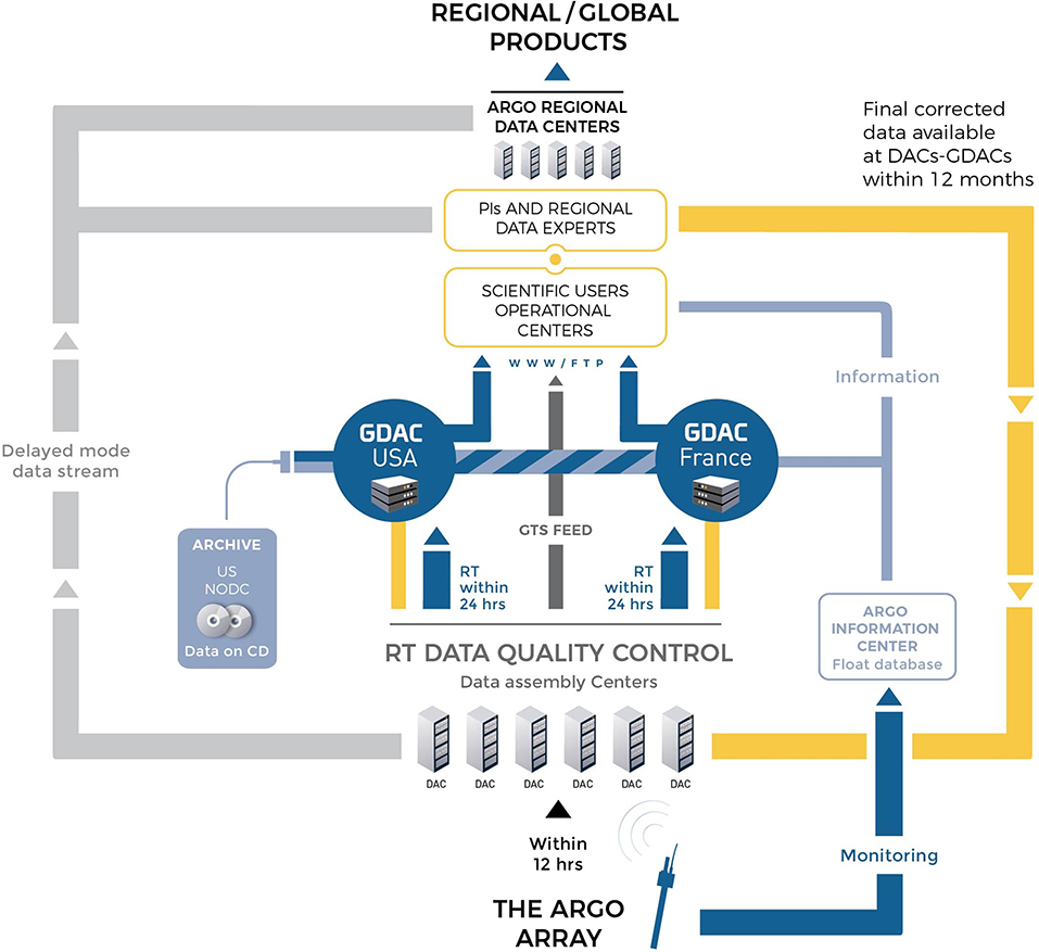
Figure 4. Components of the Argo data system and their interactions. [Source: Euro-Argo ERIC].

Implementing an open data policy at all levels of processing has made the Argo data system a pioneer in scientific ocean data delivery. Data are publicly and freely available via two Global Data Assembly Centers (GDACs): the Coriolis Data Center in France and the US Navy's Fleet Numerical Meteorology and Oceanography Center (FNMOC). Data are available in a common netCDF format and can be downloaded by File Transfer Protocol (FTP) or via a World Wide Web (WWW) interface. The two Argo GDACs receive data that have been processed by 11 national Data Assembly Centers (DACs). Each float is allocated to a specific DAC. Functions of a DAC, as described below, may be centralized at a single institution or spread across several as appropriate. Data holdings at the two Argo GDACs are synchronized once per day. The two GDACs are access points for all Argo data.

At the GDACs, data from each float are stored in 4 types of files:

• a metadata file that holds the float's specifications and sampling configurations, which can vary in time for Iridium floats;

• a technical data file that stores transmitted engineering information;

• a trajectory data file that stores positions, cycle timing, surface data, and park-phase data; and

• a profile data file for each float cycle that stores vertical profile data from that cycle. (For floats equipped with biogeochemical sensors, vertical profile data are stored in two separate profile data files. See section Extension of the Argo Data System.)

A file checker operated at the GDACs checks the format and content consistency of these data files before they are admitted into the global data holdings (Ignaszewski, 2018). Moreover, for each float, the GDACs concatenate the single-cycle profile files together to make a multi-cycle profile file for each float, for users who require all profiles from each float in one file.

Vertical profile data and trajectory data are subjected to a common set of quality control procedures (Wong et al., 2020) and are available via two pathways: real-time and the slower but more accurate delayed-mode.

Real-Time

Data are received via satellite transmission, decoded and assembled at national DACs. These DACs apply a set of automatic quality tests to the data, and quality flags are assigned accordingly. These flags warn users about grossly bad data that may result from corrupted data transmission or sensor malfunction. Data may be adjusted automatically in real-time in a preliminary manner, based on information from the float or results from the delayed-mode procedures described below. In such cases both the raw and real-time adjusted data are provided to users. The formatted and flagged data are passed on to the two Argo GDACs in netCDF files, as well as inserted onto the Global Telecommunications System (GTS) in the Binary Universal Form for the Representation (BUFR) format. The BUFR format replaced the earlier TESAC code form in 2018, which did not allow the inclusion of quality flags. The GTS channel is mainly used by operational meteorological agencies. Available within <24 h of satellite transmission, the real-time data are used for operational weather and ocean forecasting, data assimilation, and other applications that require timely data that are not necessarily of final and highest possible quality.

Delayed-Mode

In the delayed-mode process, data are subjected to visual examination by oceanographic experts and are re-flagged where necessary, as the real-time automatic procedures are not flawless. Float data can also be affected by sensor drift, but because retrieving floats for recalibration is rarely possible, statistical tools and climatological comparisons are used to adjust the data for sensor drift when needed. Determination of sensor drift requires accumulation of a relatively long time series. In Argo, the usual practice is to examine the profiles in delayed-mode initially about 12 months after they are collected, and then revisit several times as more data from the floats are obtained, until the floats become inactive. Thus, the most recent version of the global dataset should be used whenever possible to take advantage of these activities. The delayed-mode pathway aims to provide the highest-quality version of the data and includes realistic error estimates. Both the raw and adjusted versions of the data are retained, as well as comments on what adjustments have been made to the data. Delayed-mode quality data are suitable for use in scientific applications that require high accuracy, such as climate research.

In order to enhance the real-time and delayed-mode pathways for detecting data errors, three additional independent global analyses have been added to the Argo data system. First, since 2010, a satellite altimetry comparison is performed every 3 months at CLS, France, in partnership with the French GDAC at Coriolis. For each float time series, the steric heights from Argo profiles are compared with independent and contemporaneous (i.e., collocated in time and space) satellite altimetric height estimates (Guinehut et al., 2009). The comparison provides an overview of the behavior of the time series of the floats and can detect outliers in the float measurements, including those that may be affected by sensor drift or calibration offsets. Second, a statistical procedure for detecting outliers by exploiting mapping error residuals is performed daily at Coriolis (Gaillard et al., 2009). This method detects float data that are not consistent with their neighbors in time and space. And third, since 2019, a daily MIN-MAX test (Gourrion et al., 2020) has been implemented at Coriolis to compare float profiles with a climatology of minimum and maximum values computed from Argo delayed-mode data and high-quality CTD data. This aids in the identification of sensor drift at an early stage. Results of these global analyses are sent to the DACs regularly, where the anomalies are flagged or adjusted by expert examination.

Since 2013, regional reanalysis of delayed-mode salinity data has been performed regularly at Coriolis. For each float that has been processed in delayed-mode, the OWC method (Owens and Wong, 2009; Cabanes et al., 2016) is run with four different sets of spatial and temporal decorrelation scales and the latest available reference dataset. If the salinity adjustments obtained from the four runs all differ significantly from the existing adjustment, then the salinity data from the float are re-examined and a new adjustment is suggested if necessary. This step has been proven to be effective in increasing consistency of delayed-mode salinity adjustments for floats in the North Atlantic Ocean.

The final component of the Argo data system is a network monitoring system developed by JCOMMOPS. This was developed as a float tracking service to ensure compliance with Intergovernmental Oceanographic Commission (IOC) resolutions regarding Argo, and subsequently expanded. It monitors the status of data availability at the GDACs and provides Key Performance Indicators on the implementation of the data system.

Extension of the Argo Data System

The Argo data system has had to expand its capacity in response to the advent of new capabilities of the profiling floats. In 2014, the Argo data system underwent a major format change to manage mission changes due to two-way communications via Iridium, to better accommodate biogeochemical profiles, to cope with different vertical sampling schemes, and to store more metadata (Argo Data Management Team, 2019). A large effort was put into homogenizing the metadata and technical data files to facilitate comparisons of float and sensor models, tracking of the health of the array, and identifying of floats with potentially bad sensors by serial numbers. The trajectory data files were revamped to include more information about the events during a float mission cycle and the times associated with these events. The profile data files were re-formatted to allow multiple profiles from a single sampling cycle (instead of the traditional limit of one profile per cycle). The ability to store multiple profiles within one cycle has allowed the addition of biogeochemical data and other specialized data, such as the un-pumped temperature measurements, in the profile data files.

The Argo Program presently consists of three elements: Core, Biogeochemical (BGC), and Deep (Figure 5). Core-Argo is concerned with the standard mission of sampling CTD data from 0 to 2,000 dbar every 10 days. Deep-Argo aims to sample temperature and salinity over the full ocean depth up to 6,000 dbar. BGC-Argo is based on integrating new sensors onto standard float platforms to measure six BGC ocean variables: chlorophyll fluorescence, particle backscatter, dissolved oxygen, nitrate, pH, and irradiance, in addition to temperature and salinity. While Deep-Argo profiles require some increase in data management effort in terms of data processing and new quality control procedures, the introduction of BGC float data into the Argo data system has generated multiplicative challenges due to their complexity (Bittig et al., 2019). To minimize the impact of adding BGC data to the Argo data streams, the CTD and BGC data are stored in two separate profile data files: a Core-profile file, which contains the CTD data, and a BGC-profile file, which contains all the measured intermediate BGC parameters as well as the computed ocean state variables. Moreover, a synthetic profile file (the S-profile file) is generated by the GDACs to align the CTD and BGC parameters obtained with different vertical sampling schemes (Bittig et al., 2020). This vertical interpolation step is necessary because measurements from multiple BGC sensors are not always aligned during onboard processing by the floats. The S-profile file contains both the CTD and BGC data (without the intermediate parameters) and is a good product for users who want to study these BGC parameters as co-located measurements.

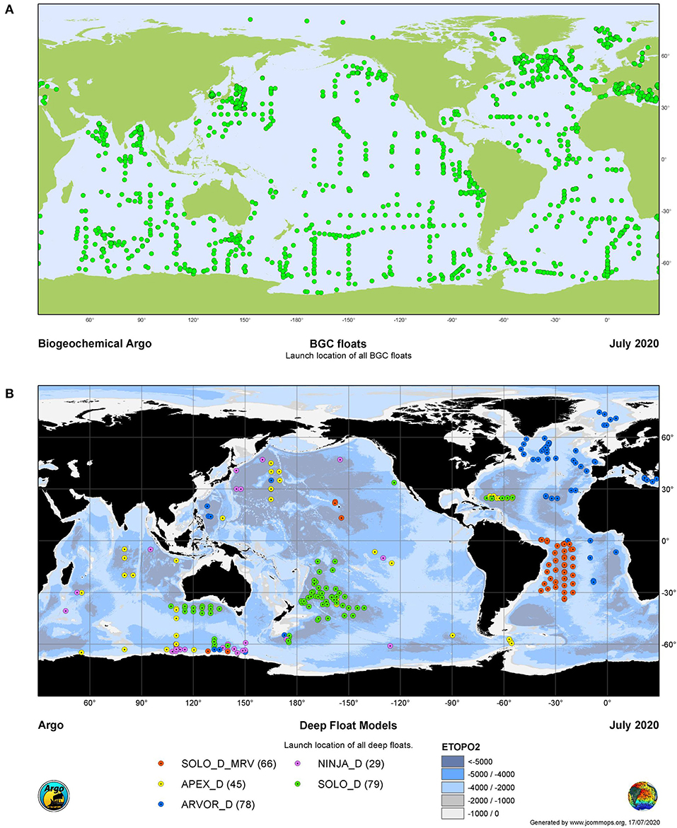
Figure 5. Global map of all (A) BGC-Argo floats, and (B) Deep-Argo floats, as of July 2020. The locations shown are the launch location of the floats. [Source: JCOMMOPS].

Lastly, to facilitate the development of experimental sensors and to satisfy the requirement that all measurements from a float are publicly available, an auxiliary directory has been established at the GDACs to distribute data from experimental sensors (e.g., passive acoustic listeners). The format of the data in the auxiliary directory is determined and documented by the float provider.

Argo Data Description

CTD Profile Vertical Resolution, Pressure Ranges, and Geographical Coverage

Vertical Resolution

The Argo CTD profile vertical resolution has been changing slowly in the past 20 years as float-providing groups switched to using Iridium for data telemetry (Figure 6). In the early days when only ARGOS telemetry was available, data transmission was limited to about 256 bytes of data per ARGOS message, which in turn limited the number of P-T-S triplets that could be transmitted per profile. Due to this data transmission limitation, and also as a means to conserve battery energy, early APEX floats used the SBE-41, which operated in the spot-sampling mode and returned low-resolution vertical profiles that typically contained about 50 to 80 discrete samples per 2,000-dbar profile. Early SOLO and PROVOR floats used the SBE-41CP and operated in the continuous-profiling mode, but yielded roughly the same number of sampling levels as the SBE-41, as the continuous data from the SBE-41CP were bin-averaged in coarse depth bins for ARGOS telemetry. With the transition to Iridium telemetry, continuous data from the SBE-41CP are averaged in smaller depth bins (typically 1-dbar or 2-dbar bins) to make good use of the increased data transmission capability, thus giving profiles with higher vertical resolutions. APEX floats subsequently switched to using the SBE-41CP as well.

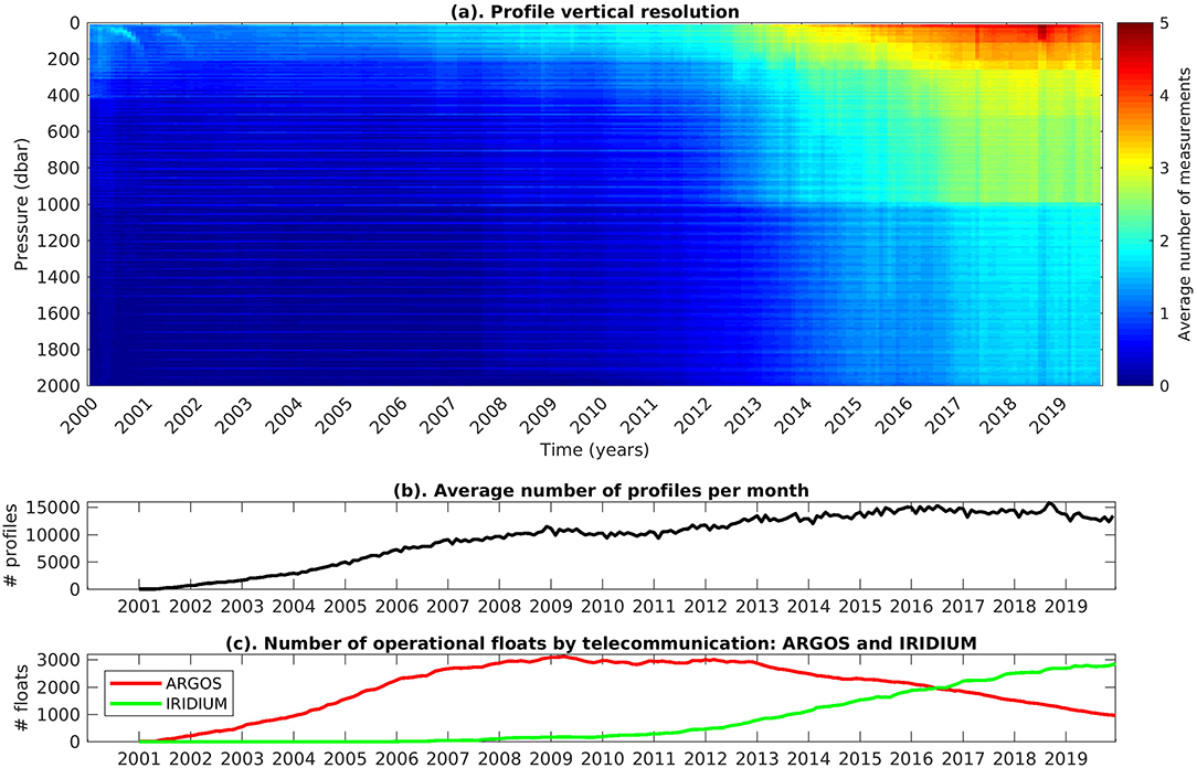
Figure 6. (a) Changes in Argo CTD profile vertical resolution from year 2000 to 2019. The color bar indicates the number of measurements divided by the number of profiles in every 10-dbar bin and in every month, averaged over each year. (b) The average number of total Argo profiles per month. (c) The number of ARGOS and Iridium floats. Note that the increase in vertical resolution is due to the increase in Iridium floats.

The SBE-41CP can operate in both the spot-sampling mode and the continuous-profiling mode. Some float operators prescribe a “mixed” vertical scheme that typically involves sampling the deeper (e.g., below 1,000 dbar), less variable part of the vertical profile in the low-resolution spot-sampling mode, and the shallower, more variable part of the vertical profile in the high-resolution CP mode. This “mixed” vertical sampling scheme is mainly used for the purpose of conserving the battery energy of the floats, especially those that are equipped with biogeochemical sensors (Riser et al., 2018). Table 1 gives an overview of the primary vertical sampling schemes used by the various float types in Argo as of 2019.

Pressure Ranges

The distribution of pressure ranges of Argo floats has also been changing over the past 20 years following the increase in float capability to profile to greater depths (Figure 7). Most early float models were only capable of profiling from shallower pressures (1,000, 1,200, or 1,500 dbar), particularly in the tropical oceans due to limited buoyancy generation and battery energy. As the buoyancy issue was resolved and floats became capable of profiling from as deep as 2,000 dbar, some floats adopted a scheme of only sampling from 2,000 dbar every 3rd or 4th profile (and from shallower pressures for other profiles) to save battery energy. Float lifetimes are ultimately limited by battery exhaustion, and many Argo floats were originally deployed with alkaline batteries. Over time, the use of lithium batteries became more common, and most floats now use them. Lithium batteries have more than twice the energy density of alkalines, hence considerably extending float lifetimes. Presently, with the transition from alkaline to lithium batteries, and the increased capacity of the buoyancy engines, modern Argo floats operate to pressures of 2,000 dbar on nearly every profile. Some new models of floats may have sufficient battery energy for 10 years of 10-day cycling to 2,000 dbar.

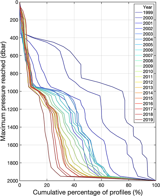
Figure 7. Cumulative percentage of Argo profiles that reached a given pressure (in 50-dbar intervals from 0 to 2,000 dbar) in each year from 1999 to 2019. For example, the percentage of profiles that sampled to at least 1,600 dbar increased from only 10% in 1999 to 80% in 2019.

In recent years, float models have been developed that are capable of 4,000 dbar and 6,000 dbar operations over a duration of several years (Roemmich et al., 2019). Improvements have also been made to the accuracy and stability of the CTDs used on these deep floats, so that they are suitable for sampling the small temperature and salinity signals of the abyssal oceans. In 2016, the first Argo profiles deeper than 2,000 dbar became available. These technological developments have enabled the formulation of the Deep-Argo program, which will extend Argo's sampling pressure ranges to full-ocean depths except over the deepest abyssal plains and trenches.

For most profiling floats, the CTD pump is normally switched off at around 5 dbar during ascent, in order to avoid contamination of the conductivity cell from the ingestion of material on the sea surface. Some floats now profile to within 2 dbar of the sea surface, as the pressure sensors have become more accurate and thus the risk of surfacing with the CTD pump on is much less. Several float types also continue to sample up to the sea surface with the pump off, or carry auxiliary modules for high-resolution near-surface sampling.

Geographical Coverage

The geographical coverage of Argo has expanded over the past 20 years largely due to the use of Iridium communications (Figure 3). ARGOS floats deployed in the equatorial region (5°S−5°N) tended to disperse poleward via Ekman transport while on the sea surface. Similarly, ARGOS floats in marginal seas or in near-coastal regions tend to have a higher probability of grounding because their prolonged surface times expose them to more cross-bathymetric wind transport. With their short surface times, Iridium floats are subjected to less Ekman divergence and wind transport, and therefore tend to disperse less in the equatorial and near-coastal regions.

The use of Iridium has also enabled the geographical coverage of year-round Argo data to expand to the seasonal sea ice zones in the Southern Ocean (Wilson et al., 2019) and in the Arctic Ocean (Smith et al., 2019). Early attempts to sample the ice-covered polar oceans showed high instrument mortality rates, either because of crushing between ice floes at the sea surface or hitting the bottom of the ice packs during ascent. However, the inclusion of a robust ice avoidance algorithm in the float software has enabled floats to operate more successfully in the seasonal sea ice zones without additional hardware requirements. The ice avoidance algorithm (originally called the ice sensing algorithm, ISA) was first developed at the Alfred Wegener Institute (AWI) for Polar and Marine Research, and was based on the assumption that the likelihood of the presence of sea ice was related to the temperature of the water column below (Klatt et al., 2007). In practice, the algorithm computes the median temperature of the near-surface mixed layer between depths Z₁ and Z₂ as the float ascends. If the median temperature is less than a prescribed threshold T_ref, the presence of sea ice is assumed, and the float will abort its ascent to the sea surface, store the profile data onboard, and descend to park pressure to begin its next cycle. For floats that use the Iridium satellite system for data communication, under-ice profiles that are collected and stored onboard the floats during winter are transmitted when surface conditions become ice-free during early summer (Riser et al., 2018).

The ice avoidance algorithm was first implemented by AWI on floats in the Weddell Sea in 2002 (Klatt et al., 2007). The first AWI algorithm set Z₁ = 50 m, Z₂ = 20 m, and T_ref = −1.79°C. In 2007, the University of Washington began deploying floats around the Antarctic continent with a version of the AWI algorithm modified for use with Iridium communication (Wong and Riser, 2011). Presently the ice avoidance algorithm is a feature in the float software of several float types. As of December 2019, more than 18,000 Argo CTD profiles have been collected from under winter sea ice around the Antarctic continent.

In the Arctic Ocean, the French-Canadian Green Edge Project has successfully deployed PROVOR/ARVOR floats with the ice avoidance algorithm in Baffin Bay (Smith et al., 2019). The PROVOR/ARVOR floats are able to overcome the strong pycnocline in the Arctic Ocean because of their large oil reserve. For the Arctic Ocean, the parameters of the algorithm were set to Z₁ = 30 m, Z₂ = 10 m, and T_ref = −0.5°C initially, with T_ref subsequently changed to −1.1°C or −1.3°C, based on sea conditions. Other Euro-Argo projects, such as the Monitoring the Oceans and Climate Change with Argo (MOCCA) project, have also deployed floats in the Arctic Ocean by using the ice avoidance algorithm with parameters tuned to local conditions.

An examination of a map of Argo's geographical sampling density indicates that there is a weak bias toward sampling near coasts with major population centers (e.g., the western North Pacific, the western North Atlantic, and near Australia), likely due to the ease of deploying in these regions. This bias does not appear to be severe or likely to affect global statistics derived from the data. With the increase in deployments in the Southern Ocean in recent years, especially resulting from the Southern Ocean Carbon and Climate Observations and Modeling (SOCCOM) program (Riser et al., 2018), and the reduction in float divergence at low latitudes resulting from the use of Iridium communication, Argo is improving its geographical coverage in regions that are historically sparse in observations due to difficult logistics.

Temperature: Accuracy and Issues

Manufacturer Static Calibration

Temperature sensors in SBE CTDs are calibrated with respect to the International Temperature Scale of 1990 (ITS-90) in stable, computer-controlled calibration baths. The basis of temperature calibration in the Sea-Bird Scientific metrology lab are two NIST-certified primary standards: the Jarrett triple-point of water cell (0°C) and the Isotech gallium melt cell (29.76°C). These physical standards provide temperature measurements with precision to 5 × 10⁻⁵ °C and accuracy to 0.0005°C. These standards are then transferred via a standardized, traceable procedure to the calibration baths, yielding static accuracy of 0.002°C for the SBE-41/41CP CTDs.

Long-Term Sensor Stability

At Sea-Bird Scientific, long term stability for temperature sensors in the SBE-41/41CP is determined from repeat multi-year laboratory calibrations of a reference set of sensors, which yield a typical stability of 0.0002°C yr⁻¹. Long-term sensor stability in the field is more difficult to assess than in the laboratory, as there are very few opportunities to retrieve floats from the ocean for post-deployment calibrations. Oka (2005) performed one such study. They investigated the long-term stability of the temperature sensors on the SBE-41 using 3 recovered floats. The floats were deployed by JAMSTEC and were in operation in the North Pacific Ocean for 2–2.5 years. They calculated differences from pre- and post-deployment sensor calibration by using an SBE-3 standard temperature sensor and an SBE-41 calibration bath system in JAMSTEC. Their results showed positive temperature changes of 1.36 (±0.62), 1.58 (±0.88), and 1.00 (±0.93) × 10⁻³ °C, respectively. Hence, although temperature sensor drifts were detected, the amounts of drift were <0.002°C over several years.

In another study, Janzen et al. (2008) assessed temperature sensor stability in the SBE-41 based on experiments in the laboratory and on recovered floats. They conducted repeat calibrations on two SBE-41 CTDs over 5 years and post-calibrations on 6 recovered floats that had been in operation for 2–6 years. They reported that from the repeat calibrations on the two SBE-41 CTDs, the standard deviation of temperature measurements was 0.001°C, and from the pre- and post-calibrations on the 6 recovered floats, negative sensor drifts of no > −0.002°C.

Currently the Argo delayed-mode QC procedure for temperature relies on visual inspection of float temperature profiles against nearby data to detect errors. After delayed-mode inspection, float temperature data are given the manufacturer quoted accuracy of 0.002°C.

Pressure: Accuracy and Issues

Manufacturer Static Calibration

All strain gauge pressure sensors used on SBE CTDs for Argo floats are calibrated at Sea-Bird Scientific. Calibrations spanning both temperature and pressure ranges are necessary, as strain gauge pressure sensors have a nominally linear response to pressure and a secondary, non-linear response to temperature. The pressure-span calibration is performed by using automated dead-weight testers. The pressure sensors measure absolute pressure, which is converted to gauge pressure by subtracting mean atmospheric pressure (equivalent to 14.7 pounds per square inch absolute).

Laboratory pre-deployment testing data from Argo teams indicate that the Druck pressure sensor displays a negative bias at cold temperatures that is a function of pressure. Therefore, in order to satisfy the accuracy requirements of the Argo Program, an additional temperature span calibration is performed at Sea-Bird Scientific. This extended calibration range improves the span correction at high pressures and low temperatures from ± 4 to ± 2 dbar for the 2,000-dbar sensors. Repeat calibrations of 10 sensors returned to Sea-Bird Scientific after more than a year after their initial calibration showed shelf drift of ± 0.30 dbar per year.

Long-Term Sensor Stability

The long-term stability of the pressure sensors can be evaluated by checking the time series of sea surface pressure (SP) values that are used in delayed-mode pressure adjustments. Floats normally collect at least one SP measurement at the end of each cycle while transmitting data at the sea surface. These SP readings are gauge pressures at sea level and are mostly within 1 dbar of zero if the pressure transducer is stable. Therefore, any pressure sensor drift will be seen in the SP readings and can be eliminated by subtracting SP from the measured pressures (Barker et al., 2011). This pressure adjustment is done onboard automatically for some float types (the auto-correcting floats, e.g., SOLO, PROVOR), but is done as part of the real-time and delayed-mode adjustment process for other float types (the non-auto-correcting floats, e.g., APEX, NAVIS).

APEX floats, one of the non-auto-correcting float types in Argo, report the raw pressure measurements and the SP values separately. Thus, examining the SP values from APEX floats is an effective way to gauge the long-term stability of pressure data from the SBE CTDs. Analysis of delayed-mode pressure data from 2,779 APEX floats showed that over the course of 280 cycles, about 5% of the SBE CTDs showed pressure sensor drift > 2.4 dbar, and only about 3% showed pressure sensor drift > 5 dbar (Figure 8).

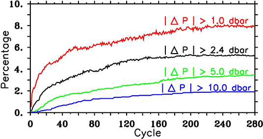
Figure 8. Percentage of pressure adjustments vs. the number of cycles, from 2,779 APEX floats.

After delayed-mode adjustment, float pressure data are given the accuracy of 2.4 dbar, which is historically (before 2011) the manufacturer's quoted accuracy for pressure. The method of using SP values to adjust pressure can eliminate the depth-independent error (the offset error) in long-term sensor drift, but cannot account for any depth-dependent error (the slope error). However, comparisons against ship-based CTD data show that the median of possible depth-dependent pressure bias in the Argo profiles is within the manufacturer quoted accuracy of 2.4 dbar, as will be discussed in section Assessment of Pressure Bias below.

Problems Encountered

Pressure measurements from Argo floats have been affected by several major sensor issues over the past 20 years (Barker et al., 2011). In 1999–2000, SBE CTDs were fitted with pressure transducers manufactured by the Paine Corporation. These were discontinued because they showed significant instrument drift over the course of a float's lifetime (e.g., Gouretski and Koltermann, 2007). Pressure transducers from Ametek were then employed during 2000–2002, but were then discontinued when a manufacturing defect, which also caused significant instrument drift over time, was discovered. Beginning in 2002, SBE used Druck pressure transducers. While the Druck pressure sensors typically produce stable measurements, two episodes of manufacturing defects affected one generation of Argo floats. These are the Druck “snowflakes” problem and the Druck “microleak” problem. The Druck “snowflakes” problem was due to internal electrical shorting by titanium oxide particles (“snowflakes”) in the oil-filled cavity in the pressure sensor, causing erratic pressure measurements and thus erratic temperature and salinity measurements. The Druck “microleak” problem occurred when oil leaked through fine cracks in the glass/metal seal of the inner chamber of the sensor, causing an internal volume loss and thus an increasing negative offset at all pressures. These problems no longer occur: Druck has rectified the “snowflakes” problem and SBE has implemented procedures that can screen for “microleaks”. Figure 9 shows the typical pressure sensor drift patterns from the Ametek, Paine and Druck sensors, and an example of a Druck sensor suffering an oil microleak. In 2010, due to a supply constraint of Druck sensors, SBE started fitting some CTD units with Kistler pressure sensors. Presently, SBE use pressure sensors from two manufacturers: Druck and Kistler (<10% Kistler as of April 2020).

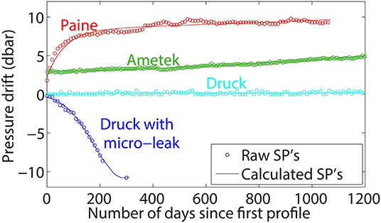
Figure 9. Typical SP offsets (dbar) for pressure sensors: Paine (WMO ID 56501), Ametek (WMO ID 2900089), Druck (WMO ID 3900263), and a Druck microleaker (WMO ID 5901649). [Source: from (Barker et al., 2011). Copyright 2011 American Meteorological Society (AMS)].

Controller board issues have also affected some float pressure measurements. In some APEX floats, the SP values were restricted to greater than zero. This was done as part of the mission control to turn off the CTD pump as the float neared the surface. These are APEX floats with controller boards identified as APF8 or earlier series. On these APEX floats, negative SP values are truncated to zero before telemetry. Thus, as a result of this onboard truncation, negative pressure drifts cannot be identified and therefore cannot be corrected. These data are labeled as having possible Truncated Negative Pressure Drifts (TNPDs), and account for about 5% of all Argo CTD profiles. Some APF8 controller boards were updated specifically to remove this “truncating” feature. All later series of controller boards on APEX floats, APF9 and above, return raw SP values with no truncation of negative values.

Another pressure problem that has affected Argo data results from processing errors onboard the floats. In 2007, it was discovered that some SOLO floats from the Woods Hole Oceanographic Institution (designated as SOLO-W) returned incorrect pressure values because of a bin-average error in the firmware. As a result, profile data from these SOLO-W floats are offset upward by one or more pressure levels, resulting in a cold bias at depth from these instruments (Willis et al., 2009). Data from the affected instruments have been identified and flagged as bad in the Argo dataset, and account for about 1% of all Argo CTD profiles. These affected SOLO-W floats are no longer active.

Salinity: Accuracy and Issues

Manufacturer Static Calibration

The SBE-41/41CP are calibrated as a complete unit such that the conductivity calibration is run concurrently with the temperature calibration. During the calibration process, an SBE-4 conductivity sensor is used as the reference sensor in the calibration bath. At the 24.0°C calibration, the bath salinity is checked with an Autosal laboratory salinometer standardized to International Association for the Physical Sciences of the Oceans (IAPSO) standard seawater. The conductivity ratio of the SBE-4 reference to the Autosal is used to correct the conductivity reference over the calibration range. This procedure is repeated 3–5 times in order to assess sensor stability. Static accuracy from the calibration process is 0.0003 Siemens per meter for conductivity, which corresponds to about 0.0035 PSS-78 in salinity accuracy at 2°C and 2,000 dbar.

Sensor Response Correction

Attaining the most accurate salinity from conductivity, temperature, and pressure measurements requires considerable processing and a number of corrections for various sensor response issues (e.g., McTaggart et al., 2010). For 1 Hz or more frequently sampled data, the mismatch between the 0.5 s response time of the SBE-41CP thermistor and the faster response of the conductivity cell must be taken into account. The combined effect of the difference in sampling time between conductivity and temperature by the CTD, plus the time required for water to flow from the thermistor into the cell must also be accounted for (e.g., Johnson et al., 2007; Martini et al., 2019). However, for bin-averaged data (on order of 10 s per dbar) or spot-sampled data, these adjustments, which amount to fractions of a second, are not possible. They could be done within the CTD onboard the float prior to bin-averaging and transmission, but those corrections have not yet been implemented internally on the SBE-41/41CP.

The conductivity cell thermal mass error (e.g., Johnson et al., 2007) represents a longer (multi-second) time-scale error. The error results from the fact that the conductivity cell and its surrounding protective jacket (the covering of the conductivity cell) both store substantial amounts of heat, which they exchange among themselves, with the water outside the float (in the case of the jacket), and the water flowing through the conductivity cell. When the CTD is moving through a vertical temperature gradient, this can mean that the temperature of the water in the conductivity cell is not the same as the temperature measured by the thermistor. Since conductivity is a strong function of temperature, the temperature of the water in the cell must be estimated (and used) to attain an unbiased salinity measurement. Although the most obvious manifestation of this error is a “spike” at the base of the mixed layer, this error, left uncorrected, also causes a bias in the thermocline, and can exceed 0.01 PSS-78 in some cases.

The conductivity cell thermal mass error can be corrected in a statistical sense, in spot-sampled data and 2-dbar bin-averaged data, assuming the temperature gradients are well-characterized at the telemetered data resolution, if the ascent rate of the float is known (Johnson et al., 2007). The correction coefficients depend on the CTD type, with different coefficients for the SBE-41 and the SBE-41CP because of their different pumping strategies. The SBE-41CP pumps slowly and continuously when operated in CP mode, whereas the SBE-41 pumps faster but intermittently, turning on only for spot samples. Coefficients for the SBE-41CP in spot-sample mode have not been determined, and work is ongoing to better characterize this error (e.g., Martini et al., 2019).

Long-Term Sensor Stability

The long-term stability of float salinity data is evaluated in delayed-mode by comparing time series of data from each float with nearby high-quality reference data on potential temperature surfaces. The differences between float-measured and reference values over several years are treated by statistical methods and represented by a piecewise linear fit to discern any observable trends over time (Wong et al., 2003; Bohme and Send, 2005; Owens and Wong, 2009; Cabanes et al., 2016). The observed trends are then evaluated by oceanographic experts to determine whether they are due to sensor drift or due to ocean variability. If the observed trends are determined to be due to sensor drift, then the salinity data from the affected floats are adjusted to the reference data according to the piecewise linear fit over time. The salinity adjustment is computed as a multiplicative correction in potential conductivity, which is equivalent to an additive correction in salinity, with slight variations as a function of pressure due to the non-linearity of the equation of state for seawater. This model assumes that the changes in reported salinities are due to changes in the measurement volume of the conductivity cell (Lueck, 1990). In practice, this model works well for any salinity sensor drifts that can be adjusted with an offset correction with no significant vertical variations.

The effectiveness of this statistical method relies on availability of contemporaneous reference data and/or the existence of water masses that have stable temperature-salinity characteristics for comparison. In Argo delayed-mode salinity analysis, two separate reference databases are used: a first one that is based on shipboard CTD data, and a second one that is based on Argo profiles that have been judged as accurate and needing no adjustment. Both databases are updated periodically to include more recently-acquired reference data, so as to account for temporal changes in the global ocean.

Analysis of delayed-mode salinity data from 10,048 Argo floats showed that for the first 2 years after deployment (about 72 cycles), <10% of the floats required any kind of sensor drift adjustment (Figure 10). After 280 cycles, about 40% required salinity adjustments > 0.01 PSS-78 in magnitude, while 30% required adjustments > 0.02 PSS-78 in magnitude. With adequate reference data and stable water masses, the statistical technique used in delayed-mode can usually produce adjusted float salinity data with about 0.01 PSS-78 uncertainty. In most cases, when the magnitude of sensor drift exceeds 0.05 PSS-78, the data will become erratic or will exhibit significant vertical variations in the amount of sensor drift. These salinity data are flagged as bad and not adjustable in delayed-mode.

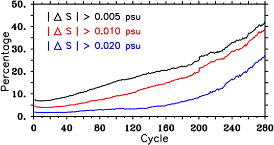
Figure 10. Percentage of salinity adjustments vs. the number of cycles, from 10,048 Argo floats.

Problems Encountered

The calibration drift of salinity sensors over time is a common problem in oceanography. Shipboard CTDs are recalibrated regularly to maintain their stability and accuracy, but this is obviously not possible for floats. Early float deployments that used the FSI inductive-style conductivity sensors with a dissolvable biocide coating showed that the cells tended to drift toward fresher values. SBE CTDs use an enclosed pumped system with the electrical conductivity of the seawater measured directly. This method of inferring salinity from conductivity produces highly accurate salinity estimates, but it relies on the geometry of the conductivity cell remaining stable and uncontaminated (Riser et al., 2008). Biocide is used in the pumped loop of the SBE conductivity cells to mitigate biological fouling on the cells. Occasionally the biocide can leak onto the cell, causing a fresh offset in salinity, but that usually gets washed away within a few sampling cycles and the salinity measurements return to being in calibration. An additional measure to prevent biofouling is to shut off the CTD pump before the instrument reaches the sea surface. As noted earlier, with the current use of Iridium telemetry, the time spent on the sea surface, where floats are most susceptible to biofouling and other hazards, is reduced (Roemmich et al., 2004).

Overall the SBE CTD design has worked well over the years, with only a minority of conductivity cells showing mild sensor drift over time. However, starting around 2015, a larger than average number of SBE CTDs in the serial number band 6000–7100 developed a drift toward higher salinities within 2–3 years of deployment (Figure 11). Many of these SBE CTDs were still active as of the time of this writing and, as a result, a higher than normal portion of Argo real-time salinity data were subject to errors that were larger than 0.01 PSS-78. The best estimate was that, at the time of this writing, about 25% of real-time profiles might be subject to this salinity error. In the real-time data stream, the Argo national DACs have flagged salinity from the SBE CTDs in the serial number range 6000–7100 as questionable data. In the delayed-mode data stream, the adjustment of these affected SBE CTDs has been treated with high priority. As a result, the residual salinity bias in the Argo dataset due to this sensor drift is now small. The cause of this conductivity drift is presently still under investigation.

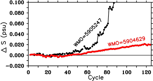
Figure 11. Two examples of SBE CTDs that showed salty sensor drift: a “slow” drift (WMO ID 5904629, in red), and a “fast” drift (WMO ID 5905247, in black).

Assessment of Argo Pressure and Salinity Bias Against GO-SHIP

Shipboard CTD systems, used with water sampling bottle salinities and recently calibrated sensor sets, deliver the highest possible accuracy data presently available. Here we have attempted to quantify any possible bias in Argo pressure and salinity by comparison with data from the Global Ocean Ship-Based Hydrographic Investigations Program (GO-SHIP). GO-SHIP grew out of the WOCE Hydrographic Program and adopted and built upon WOCE data standards. CTD data from 280 post-2000 GO-SHIP cruises were selected. Nearby Argo and GO-SHIP profile buddies, or pairs, were defined as profiles deeper than 1,300 dbar that were collected within 300 km and 30 days of each other. Individual Argo and GO-SHIP profiles could (and typically did) appear in multiple pairs, but each pairing was unique. In total, 294,373 Argo/GO-SHIP pairs were found with these search criteria, involving 31,056 unique Argo profiles. Only the highest-quality data have been selected (WOCE QC flag “2”; Argo QC flag “1”). The Argo profiles consist of both real-time profiles and delayed-mode profiles.

Argo/GO-SHIP differences were then examined on a density surface: specifically, potential density anomalies relative to 1,000 dbar (σ₁). In order to account for the wide variation in σ₁ stratification across latitudes, a separate σ₁ grid was defined for each 20° latitude band (−90° to −70°, −70° to −50°, etc.). These σ₁ grids were determined by averaging GO-SHIP σ₁ profiles in each latitude band and on 10-dbar pressure levels from the surface to 2,000 dbar. Salinity and pressure from each Argo/GO-SHIP profile pair were then interpolated onto the respective σ₁ grid based on their locations.

For each pair, a pressure difference (ΔP) and a salinity difference (ΔS) were computed from the interpolated values on the σ₁ level, where GO-SHIP values were subtracted from Argo values. Differences between Argo and GO-SHIP buddy profiles were due to short time- and space-scale ocean variability (such as mixed layer and eddy variability) and instrument error. In this analysis, we assumed the ocean variability was random and thus averaged to near zero across large numbers of pairs. Non-zero averaged differences were assumed to be due to instrumental bias.

Assessment of Pressure Bias

Profile pairs were analyzed in cohorts based on pressure sensor manufacturer. To illustrate statistical repeatability, we compared averages of ΔP as a function of pressure from 4 hemispheres: east, west, north, and south (Figure 12A). Argo profiles with Ametek and Paine pressure sensors had too few GO-SHIP buddies to deliver a statistically stable result, as medians from different hemispheres were divergent. By far the most abundant pressure sensor represented in the profile pairs was the Druck sensor. Our results showed that a slight high-pressure bias existed near 1,000 dbar, but its magnitude was within the manufacturer's stated sensor accuracy. At levels deeper than 1,200 dbar, the results were not stable statistically, as indicated by a lack of agreement between hemispheric averages. Kistler sensor results from this analysis were also noisy but suggested a slight high-pressure bias that was also near the manufacturer's stated sensor accuracy; in aggregate, across all pairs, the results were similar to those from the Druck cohort. Overall, we found no evidence of a large pressure bias for Druck and Kistler profiles, though a small bias might exist near the boundary of the historical manufacturer's stated sensor accuracy of 2.4 dbar.

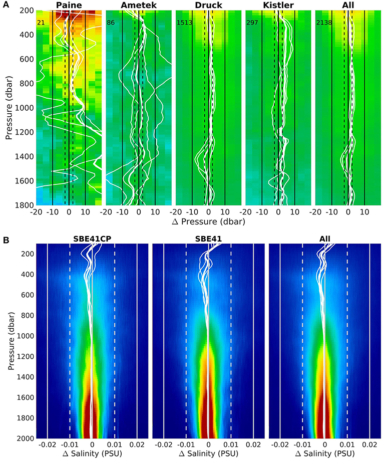
Figure 12. Bias (Argo minus GO-SHIP) on σ₁ surface as a function of pressure (dbar). The thick white line is the median for all pairs in a cohort, and the thin white lines are the medians across the 4 hemispheres: east, west, north, and south. Colors qualitatively indicate the fraction of data in a bias bin for any given pressure (high fraction in red, low fraction in blue). (A) Median pressure bias (Argo minus GO-SHIP), for buddy pairs averaged by pressure sensor makers. Black dashed lines show the manufacturer accuracy specification on deployment of 2.4 dbar. The number of floats in each buddy cohort is marked in the top left-hand corner. (B) Median salinity bias (Argo minus GO-SHIP), for buddy pairs averaged by CTD types. Gray dashed lines show expected accuracy of 0.01 PSS-78.

Assessment of Salinity Bias

A similar analysis was done for salinity differences ΔS on the σ₁ surface across the pairs. For the cohorts of CTD type for which there were enough pairs (SBE-41/41CP), any bias in the dataset was much smaller than 0.01 PSS-78 (Figure 12B). Across most of the water column, the bias was about 0.001 PSS-78 for the Druck and Kistler pressure sensor cohorts. There was a small fresh bias that peaked around −0.002 PSS-78 in the lower thermocline (400–800 dbar), but it was not evident in all the hemispheres. While GO-SHIP profiles do contribute to Argo's reference database used to assess salinity sensor drift, their small number, along with the fact that only about 15% of Argo profiles are adjusted, means that they likely do not dominate these estimates. Thus, it is remarkable that, in aggregate, Argo profiles show such small salinity bias compared to the contemporaneous GO-SHIP surveys. This result is also consistent with the small pressure bias analyzed above. For example, a pressure bias of 10 dbar will manifest as a salinity bias of 0.005 PSS-78 near 2,000 dbar, which is not evident in Figure 12.

Another way to assess float salinity accuracy is by comparing Argo salinity estimates on a deep potential temperature surface found in the ancient water masses of the deep Pacific with that measured by the GO-SHIP program (Figure 13). In the tropics and subtropics, the P18 line samples waters at 2.8°C that are low in oxygen and high in carbon isotopes, suggesting their great age and the relative absence of surface forced influences. On this isotherm, GO-SHIP salinities show very low variance between stations (<0.003 PSS-78) north of 20°S. In comparison, the Argo salinity estimates vary much more, but largely within 0.01 PSS-78 of the GO-SHIP values. The Argo values can be clumped above or below the GO-SHIP estimates, and these are associated with a single float record, suggesting that float salinity can be biased at the 0.01 PSS-78 level.

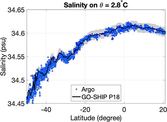
Figure 13. Salinity on the potential temperature surface of 2.8°C along the P18 GO-SHIP occupation from 2016. P18 lies roughly along 110°W in the Pacific Ocean. Black line is salinity from the GO-SHIP CTD casts, and the gray shading shows a 0.01 PSS-78 envelope around the GO-SHIP measurements. Individual Argo salinity estimates from within 1° of the GO-SHIP stations are shown in blue.

A similar study was done by Riser et al. (2008), which compared salinities from 142 floats with shipboard CTD data collected along 32°S in the South Pacific. On the 2.4°C potential temperature surface, it was found that float-derived salinities agreed with shipboard data to within 0.01 PSS-78. This salinity accuracy is in accordance with the experience of the Argo delayed-mode teams and their ability to remove sensor drift or offsets.

Positions, Subsurface Velocities, and Other Park-Phase Data

Positions

The ARGOS system uses the Doppler shift of received transmissions to estimate positions. As a result, its positioning accuracy depends on the number of satellites within range and the configuration of the constellation at the time the messages are received. ARGOS positions have four levels of accuracy ranging from better than 250-m radius to over 1,500-m radius. Some ARGOS position estimates are accompanied by an error ellipse, which gives a more exact error on individual positions than the broad horizontal error associated with the location classes.

Floats that employ the Iridium satellite system for data communications use the Global Positioning System (GPS) to establish their positions. GPS tracking is more accurate than ARGOS tracking, with a typical GPS horizontal accuracy being about 8 m (with a 95% confidence interval). Additionally, the Iridium satellite system itself can provide positions based on data from their satellites that are within range of the float. However, Iridium positions are of a much lower accuracy than GPS or ARGOS positions. Uncertainty in Iridium fixes is roughly 3 km in the meridional direction and about 20 km in the zonal direction; any individual Iridium fix can have much larger errors. Hence, Iridium positions are only used as a backup when GPS fixes cannot be obtained.

Many floats operating in the Southern Ocean are equipped with an ice-avoidance algorithm to prevent the floats from reaching the surface when sea ice is inferred to be present (see section Geographical Coverage). These under-ice profiles are stored in the memory of the floats, but they are without any satellite-derived positions. If they do not have underwater acoustic positioning capability, their positions are estimated, most commonly by linear interpolation between known positions from ice-free periods. Chamberlain et al. (2018) estimated that maximum position uncertainty over an 8-month period was 116 ± 148 km in the Weddell Sea, which was equivalent to about 1° in latitude and about 3° in longitude at 70°S.

Subsurface Velocities and Other Park-Phase Data

Computation of subsurface velocities from floats should ideally be based on the time and location of the float when it begins drifting at park pressure and the time and location when the float stops drifting and begins to descend in preparation for the ascending profile to the sea surface. Unfortunately, these positions and times are, in many cases, not well-known. The only portion of a float profile where positions are known is at the sea surface, where satellites are used to determine the float's location. Early APEX and SOLO floats transmitted some timing information, but the transmitted data were insufficient to determine both the times when the float reached the surface and when it began its descent. The first global subsurface velocity data product based on trajectories of Argo floats, YoMaHa'07, employed the last location and time on the sea surface from one cycle and the first location and time on the sea surface from the next cycle in order to make a subsurface velocity estimate (Lebedev et al., 2007). The YoMaHa'07 velocity product began with 290,247 cycles in 2007 and continued to be updated regularly. Ollitrault and Rannou (2013) used a similar method as YoMaHa'07, but with improved estimation of ascent end time and descent start time, and 600,000 deep displacements based on ARGOS and GPS fixes from floats prior to January 2010 to create the ANDRO Atlas, which continued to be updated yearly⁶. Using the ANDRO Atlas, Ollitrault and Colin de Verdière (2014) provided a gridded field of geostrophic velocities at 1,000 dbar. Gray and Riser (2014) estimated surface arrival and departure times and positions and, together with geostrophic shear estimates from profile data, created gridded absolute geostrophic velocity fields for a number of levels in the upper 2,000 dbar of the global ocean.

There are two main sources of errors in these velocity estimates: (i) unknown surface drift prior to the first and after the last location for ARGOS floats, and (ii) horizontal displacement when descending and ascending due to velocity shear. YoMaHa'07 estimated the global mean error due to both these sources to be 0.53 cm s⁻¹. Knowing that floats experience much higher currents at the surface than at depth, Park et al. (2005) tried to reduce the error due to surface drift and improve the accuracy of the subsurface velocity by using a combination of linear and circular motion at the sea surface with ARGOS float locations, along with surface arrival and departure times to estimate the corresponding positions of surface arrival and descent. They demonstrated a velocity uncertainty of the order of 0.2 cm s⁻¹ in the Sea of Japan by using this method.

In all of these efforts, the common difficulty in estimating velocities from Argo trajectory data results from a lack of timing information from the floats. In addition, for floats that use ARGOS communications, the locations at surfacing and descent are not well-known; the floats wait for unknown amounts of time at the surface prior to connecting with ARGOS satellites passing overhead in order to define a position, and then again wait for an undetermined amount of time after the last position before the float begins its descent. Newer float models that use Iridium communications return more timing information throughout the float mission, typically with a GPS fix at the beginning of the surface interval and a second GPS fix just prior to descending.

While drifting during their park phase (typically about 9 days in duration), some floats collect discrete samples of temperature, salinity, and other biogeochemical parameters. These underway data, available in the trajectory data files, have the same accuracy as the vertical profile data and have proven to be useful for studying high-frequency phenomena such as internal gravity waves (Hennon et al., 2014) and eddy diffusivity at 1,000 dbar (Roach et al., 2018).

How to Cite Argo Data: The Dynamic Doi Structure

The citation of Argo data used in scientific studies is a challenging subject since the Argo dataset is “dynamic,” evolving and growing in time. Dynamic data citation is an area of active research. To allow reproducibility of scientific studies that use Argo data, a snapshot of the entire dataset at the GDACs is preserved each month. The snapshot contains all the Argo data available at the time of the snapshot creation. To manage citation of this dynamic dataset, Argo adopted a Digital Object Identifier (DOI) format that gives a single DOI to track data usage, but that also allows users to cite specific time snapshots (Merceur, 2016). The Argo DOI takes the form http://doi.org/10.17882/42182# < nnnnn>, where < nnnnn> is the unique identifier for the specific time snapshot being used. Each snapshot identifier is appended to the DOI with a “#” character to delimit the suffix from the DOI. Based on this format, the Argo dataset can be cited in two ways:

1. The Argo GDAC as a whole (without data reproducibility) should be cited as follows: Argo Data Management Team (2019). Argo float data and metadata from Global Data Assembly Centre (Argo GDAC). SEANOE. https://doi.org/10.17882/42182.

2. An Argo snapshot (enabling data reproducibility) should be cited as follows: Argo Data Management Team (2019). Argo float data and metadata from Global Data Assembly Centre (Argo GDAC)—Snapshot of the Argo GDAC as of September 6th, 2019. SEANOE. https://doi.org/10.17882/42182#66797.

Future Challenges

While the Argo Program has made monumental progress in the past two decades on the technical problems relating to the collection of CTD data by profiling floats, work on these issues continues to this day. Individual floats now provide quality data over many years, sending megabytes of data including basic CTD parameters and a myriad of other types of observations to the GDACs, followed by adjustment of the data in a finely tuned delayed-mode process. Yet there remains room for improvement in each of these areas.

First, while many present floats provide excellent data for more than 5 years, there are still too many that fail in half of that time. While there are a number of reasons for these early failures, an all-too-often cause is the lack of adequate pre-deployment checks on the part of some float groups. A central lesson from 20 years of Argo is that there is no substitute for vigilance in making sure floats are operating properly before they are deployed. Argo has spent a considerable effort in recent years in attempting to identify and rectify these group-to-group differences. Second, while many of the CTD data returned by the floats are of good quality, there has been an alarming rise in drift in measured salinity in recent years that is still not well-understood, as noted in section Problems Encountered for Salinity. Work has been underway for several years between float deployers, data users, and manufacturers to characterize and fix this problem, and these efforts continue. In this case, as in the past with the CTD pressure sensor issues, it has been shown to be essential to monitor data quality as closely as possible and for scientists and manufacturers to remain in close communication. It is likely that there will always be sporadic problems with some components in the float and sensor supply chain that lead to compromised data quality, but the effects of such problems can be minimized with continued vigilance.

A third challenge for Argo is the delayed-mode quality control (DMQC) process of the ever-growing and diversifying dataset produced by the float array. To date, DMQC has been conducted by operators at various institutions examining each profile and determining what adjustments are necessary based on comparison with reference data. With an existing dataset comprised of over 2 million profiles, the burden placed on human resources is considerable. Argo seemingly now has an opportunity to make use of recent developments in machine learning (ML) techniques in order to improve quality control procedures, as outlined by Maze and Morrow (2017). An initial fruitful approach might be to develop automated DMQC checks on all new data, and then to direct the flow of data with problems (i.e., those not passing the explicit tests) to a ML algorithm for a second check, prior to human intervention. In such a scenario, ML could be used to sort the data, identify problems, and suggest the necessary changes, effectively reducing the workload of human operators. Such an approach has been successfully tested at Ifremer, resulting in a 25% reduction in DMQC operator workload (Maze et al., 2020). ML algorithms such as decision trees, neural networks, and Gaussian mixture models can also be used to determine the best combination of existing DMQC tests, to improve the quality of reference data (this is already in use for QC of biogeochemical Argo measurements, as noted by Bittig et al., 2018), and to improve the selection of historical profiles to be used to evaluate new, incoming data (Maze et al., 2017). In the future, advances in ML algorithms should provide an important resource to the Argo community to help to meet the challenge of maintaining the quality of its data from ever more floats and diversified missions.

Discussion and Conclusion

The original goal of the Argo Program was to provide a description of the mean state and variability in the upper 2 kilometers of the global ocean on sub-seasonal to decadal timescales. This aspiration was motivated by the success of WOCE in the 1990s to provide a first estimate of the state of the global ocean. The evolution of the float program from WOCE to Argo was not without technical challenges. The basic operation of the extant float buoyancy engine was problematic and needed redesign. The first CTD units in use performed poorly, and an effective alternative needed to be found. There was no systematic way to disseminate and manage real-time data. Furthermore, there were no agreed methods to compare data to reference datasets in order to make adjustments to measurements from floats once they were deployed. All of these issues represented daunting challenges at the turn of the 21st century.

Yet within a few years of the beginning of the Argo Program, all these technical challenges were addressed in ways that were adequate to make Argo successful. Continuing on from those early years, the Argo Program has overcome two decades of challenges because it has been supported by a multi-national team of dedicated scientists, engineers, and data experts, working in a collaborative manner. The clear goals of the Argo Program, the commitment to develop the necessary infrastructure, and the willingness to share innovative improvements in both technology and data methodology, have allowed Argo to revolutionize the way large-scale oceanographic data are collected, disseminated, and analyzed. Today, Argo is an international collaborative project that involves 34 countries. As of September 2019, data holdings at the Argo GDACs from 11 national DACs amounted to 338 gigabytes of data from 15,231 floats. The seasonal and spatial coverage of Argo is unprecedented, increasing the total available number of observed profiles in many regions from <10 per 1° square to over 50 nearly everywhere (Figure 14).

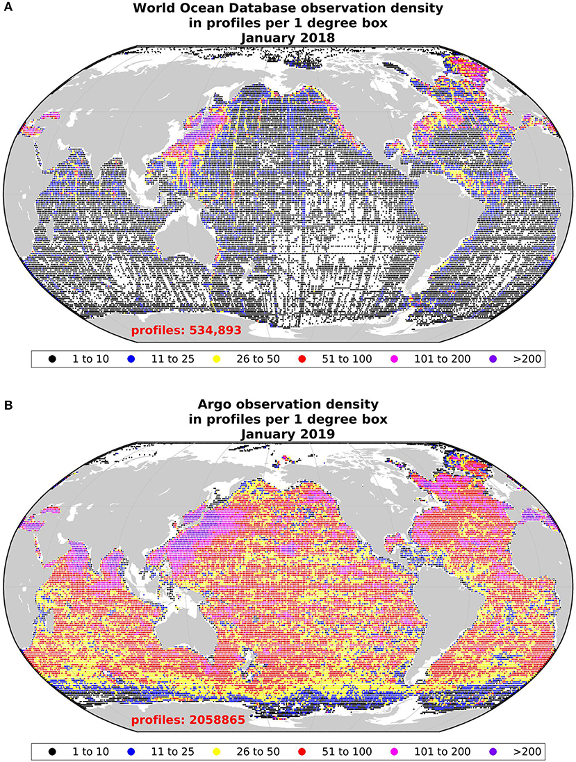
Figure 14. Total number of profiles with temperature and salinity that extend to at least 1,000 dbar for every 1° square of latitude and longitude. (A) World Ocean Database 2013 with updates from January 2018. These represent profiles collected by research or other vessels over the past 150 years. (B) Profiles collected by Argo up to January 2019.

From its inception, Argo has made its data freely available to the operational and research communities and the general public and, in doing so, has led to a new paradigm in ocean data sharing. This open-data policy, coupled with the exceptional data coverage, have driven an explosion in ocean and climate research (over 4,000 papers and 250 PhD theses have used Argo data). Argo's nearly global coverage makes it particularly useful for detection of climate change signals, for estimation of the ocean's heat content, and for observation of the intensification of the global hydrological cycle (Riser et al., 2016). Argo data also underpin ocean and climate forecasting services, through their now dominant role in ocean model initialization at most forecasting centers. After 20 years, Argo has exceeded its original aspirations. Science writer Justin Gillis of the New York Times has described Argo as “one of the scientific triumphs of the age” (Gillis, 2014).

In this paper, we have aimed to describe the core Argo dataset collected over the first 20 years of the program. When Argo was first conceived, aspirational uncertainties for the measurements of pressure, temperature and salinity were based on experience with other ocean observing programs, such as hydrographic cruises and moorings, and with the experiences acquired during WOCE. Today, we have been able to estimate accuracies of 0.002°C for temperature, 2.4 dbar for pressure, and 0.01 PSS-78 for salinity, after delayed-mode adjustments. As of 2019, the manufacturer calibration specification of salinity from the SBE-41/41CP CTDs is 0.0035 PSS-78. In reality, however, the achieved accuracy for float salinity to 2,000 dbar is closer to 0.01 PSS-78, as assessed by using independent observations from GO-SHIP measurements.

While the current accuracies in Argo data are sufficient to meet Argo's global change objectives, the program aims to improve on these. Ongoing sensor development by manufacturers and improvements in delayed-mode quality control processes will contribute to this goal. Looking forward, Argo is expanding to provide more coverage in marginal seas, more full-depth CTD profiles, and more biogeochemical measurements to study issues such as the ocean carbon cycle, deoxygenation, and ocean acidification. The future is evolving for this global ocean observing system, and the expanded vision will require similar international collaboration as over the past 20 years.

Data Availability Statement

The datasets presented in this study can be found in online repositories. The names of the repository/repositories and accession number(s) can be found in the article/supplementary material.

Author Contributions

AW, SW, SR, SP, SH, DR, JG, GJ, KM, DM, MS, TB, JB, FM, TC, GM, CC, XA, NP, IY, PB, and SG contributed to the writing of the manuscript. The remaining authors provided figures, data, and comments.

Funding

AW, SR, and other scientists at the University of Washington (UW) were supported by the US Argo Program through the NOAA Grant NA15OAR4320063 to the Joint Institute for the Study of the Atmosphere and Ocean (JISAO) at the UW. SW and other scientists at the Woods Hole Oceanographic Institution (WHOI) were supported by the US Argo Program through the NOAA Grant NA19OAR4320074 (CINAR/WHOI Argo). The Scripps Institution of Oceanography's role in Argo was supported by the US Argo Program through the NOAA Grant NA15OAR4320071 (CIMEC). Euro-Argo scientists were supported by the Monitoring the Oceans and Climate Change with Argo (MOCCA) project, under the Grant Agreement EASME/EMFF/2015/1.2.1.1/SI2.709624 for the European Commission.

Conflict of Interest

KM and DM were employed by the company Sea-Bird Scientific.

The remaining authors declare that the submitted work was conducted in the absence of any personal, professional, commercial, or financial relationships that could be construed as a potential conflict of interest.

Acknowledgments

The authors would like to acknowledge the following people who have made significant contributions to the core Argo Program in the past 20 years but who have retired or departed: Jeff Dunn, Ann Thresher—Australia; Bob Keeley, Ron Perkin—Canada; Shaohua Lin—China; Michel Arhan, Fabienne Gaillard, Catherine Lagadec, Michel Ollitrault—France; Sudheer Joseph—India; Shinya Minato, Keisuke Mizuno, Nobuyuki Shikama, Kensuke Takeuchi, Kazuhiko Hayashi, Mizuho Hoshimoto, Yoshiaki Kanno, Kensaku Kobayashi—Japan; HyunSuk Kang, SangBoom Ryoo, Moon-Sik Suk—South Korea; Stephanie Contardo, Rebecca McCreadie, Lesley Rickards, John Lawson—UK; Silvia Garzoli, Robert Molinari, Stephen Piotrowicz, Norge Larson—USA.

We wish to thank the many individuals who have contributed to float design, fabrication, testing, and deployment. In particular, John Hunt (NIWA) is acknowledged for his exceptional contribution to float deployment from the RV Kaharoa voyages.

Argo data are collected and made freely available by the International Argo Program and the national programs that contribute to it. (10.17882/42182). This paper is PMEL Contribution Number 5102.

Footnotes

References

André, X., Moreau, B., and Le Reste, S. (2015). Argos-3 satellite communication system: implementation on the arvor oceanographic profiling floats. J. Atmos. Ocean. Technol. 32, 1902–1914. doi: 10.1175/JTECH-D-14-00219.1
Argo Science Team (1998). On the design and implementation of argo - a global array of profiling floats. International CLIVAR Project Office.
Barker, P. M., Dunn, J. R., Domingues, C. M., and Wijffels, S. E. (2011). Pressure sensor drifts in Argo and their impacts. J. Atmos. Ocean. Technol. 28, 1036–1049. doi: 10.1175/2011JTECHO831.1
Bittig, H., Wong, A., and Plant, J. (2020). BGC-Argo Synthetic Profile File Processing and Format on Coriolis GDAC (Brest: Ifremer) 6:502. doi: 10.13155/55637
Bittig, H. C., Maurer, T. L., Plant, J. N., Schmechtig, C., Wong, A. P. S., Claustre, H., et al. (2019). A BGC-Argo guide: planning, deployment, data handling and usage. Front. Marine Sci. 6:502. doi: 10.3389/fmars.2019.00502
Bittig, H. C., Steinhoff, T., Claustre, H., Fiedler, B., Williams, N. L., Sauzède, R., et al. (2018). An alternative to static climatologies: robust estimation of open ocean CO2 variables and nutrient concentrations from T, S, and O2 data using bayesian neural networks. Front. Marine Sci. 5:328. doi: 10.3389/fmars.2018.00328
Bohme, L., and Send, U. (2005). Objective analyses of hydrographic data for referencing profiling float salinities in highly variable environments. Deep Sea Res. Part II. 52, 651–664. doi: 10.1016/j.dsr2.2004.12.014
Cabanes, C., Thierry, V., and Lagadec, C. (2016). Improvement of bias detection in Argo float conductivity sensors and its application in the North Atlantic. Deep Sea Res. Part I 114, 128–136. doi: 10.1016/j.dsr.2016.05.007
Chamberlain, P. M., Talley, L. D., Mazloff, M. R., Riser, S. C., Speer, K., Gray, A. R., et al. (2018). Observing the ice-covered Weddell Gyre with profiling floats: position uncertainties and correlation statistics. J. Geophys. Res. 123, 8383–8410. doi: 10.1029/2017JC012990
Davis, R. E. (1998). Preliminary results from directly measuring middepth circulation in the tropical and South Pacific. J. Geophys. Res. 103, 24619–24639. doi: 10.1029/98JC01913
Davis, R. E., Sherman, T. J., and Dufour, J. (2001). Profiling ALACEs and other advances in autonomous subsurface floats. J. Atmos. Ocean. Technol. 18, 982–993. doi: 10.1175/1520-0426(2001)018<0982:PAAOAI>2.0.CO;2
Davis, R. E., Webb, D. C., Regier, L. A., and Dufour, J. (1992). The autonomous lagrangian circulation explorer (ALACE). J. Atmosp. Ocean. Technol. 9, 264–285. doi: 10.1175/1520-0426(1992)009<0264:TALCE>2.0.CO;2
Fofonoff, N. P., and Millard, R. C. Jr. (1983). Algorithms for Computation of Fundamental Properties of Seawater. Paris: UNESCO Technical Papers in Marine Science.
Gaillard, F., Autret, E., Thierry, V., Galaup, P., Coatanoan, C., and Loubrieu, T. (2009). Quality control of large Argo data sets. J. Atmos. Ocean. Technol. 26, 337–351. doi: 10.1175/2008JTECHO552.1
Gillis, J. (2014). In the Ocean, Clues to Change. New York, NY: New York Times. Accessed: August 12, 2014.
Gould, W. J. (2005). From Swallow floats to Argo - the development of neutrally buoyant floats. Deep Sea Res. II 52, 529–543. doi: 10.1016/j.dsr2.2004.12.005
Gouretski, V., and Koltermann, K. P. (2007). How much is the ocean really warming? Geophys. Res. Lett. 34:L01610. doi: 10.1029/2006GL027834
Gourrion, J., Szekely, T., Killick, R., Owens, W. B., Reverdin, G., and Chapron, B. (2020). Improved statistical method for quality control of hydrographic observations. J. Atmosp. Ocean. Technol. 37, 789–806. doi: 10.1175/JTECH-D-18-0244.1
Gray, A. R., and Riser, S. C. (2014). A global analysis of Sverdrup balance using absolute geostrophic velocities from Argo. J. Phys. Oceanogr. 44, 1213–1229. doi: 10.1175/JPO-D-12-0206.1
Guinehut, S., Coatanoan, C., Dhomps, A. L., Le Traon, P. Y., and Larnicol, G. (2009). On the use of satellite altimeter data in Argo quality control. J. Atmos. Ocean. Technol. 26, 395–402. doi: 10.1175/2008JTECHO648.1
Hennon, T. D., Riser, S. C., and Alford, M. H. (2014). Observations of internal gravity waves by Argo floats. J. Phys. Oceanogr. 44, 2370–2386. doi: 10.1175/JPO-D-13-0222.1
Ignaszewski, M. (2018). Description of the Argo GDAC File Checks: Data Format and Consistency Checks (Brest: Ifremer). doi: 10.13155/46120
Janzen, C., Larson, N., Beed, R., Anson, K., and Sea-Bird Electronics, Inc. (2008). Accuracy and Stability of Argo SBE 41 and SBE 41CP CTD Conductivity and Temperature Sensors. Seattle: Sea-Bird Scientific Technical Papers.
Johnson, G. C., Toole, J. M., and Larson, N. G. (2007). Sensor corrections for Sea-Bird SBE-41CP and SBE-41 CTDs. J. Atmosp. Ocean. Technol. 24, 1117–1130. doi: 10.1175/JTECH2016.1
Klatt, O., Boebel, O., and Fahrbach, E. (2007). A profiling float's sense of ice. J. Atmos. Ocean. Technol. 24, 1301–1308. doi: 10.1175/JTECH2026.1
Lebedev, K. V., Yoshinari, H., Maximenko, N. A., and Hacker, P. W. (2007). YoMaHa'07: Velocity Data Assessed From Trajectories of Argo Floats at Parking Level and at the Sea Surface. Honolulu, HI: IPRC Technical Note.
Loaec, G., Cortes, N., Menzel, M., and Moliera, J. (1998). “PROVOR: a hydrographic profiler based on MARVOR technology,” in IEEE Oceanic Engineering Society, OCEANS'98. Conference Proceedings (Cat. No. 98CH36259) (Nice), 42–45.
Lueck, R. (1990). Thermal inertia of conductivity cells: Theory. J. Atmos. Ocean. Technol. 7, 741–755. doi: 10.1175/1520-0426(1990)007<0741:TIOCCT>2.0.CO;2
Martini, K. I., Murphy, D. J., Schmitt, R. W., and Larson, N. G. (2019). Corrections for pumped SBE 41CP CTDs determined from stratified tank experiments. J. Atmos. Ocean. Technol. 36, 733–744. doi: 10.1175/JTECH-D-18-0050.1
Maze, G., Mercier, H., and Cabanes, C. (2017). Profile classification models. Mer. Ocean J. 55, 48–56.
Maze, G., and Morrow, R. (2017). “Ocean and big data,” in Les Big Data à découvert, eds M. Bouzeghoub and R. Mosseri (CNRS) Paris, 368.
Maze, G., Tokunaga, S., Le Guen, R., and Carval, T. (2020). Machine Learning and Ocean Data Quality Control. Paris: MOCCA General Assembly.
McTaggart, K. E., Johnson, G. J., Johnson, M. C., Delahoyde, F. M., and Swift, J. H. (2010). “Notes on CTD/O2 data acquisition and processing using Seabird hardware and software (as available),” in GO-SHIP Repeat Hydrography Manual: A Collection of Expert Reports and Guidelines, eds E. M. Hood, C. L. Sabine, and B. M. Sloyan (IOCCP), 1–10.
Merceur, F. (2016). DOIs for Ocean Data, General Principles and Selected Examples (Argo, French cruises) (Brest: Ifremer). doi: 10.13155/44515
Oka, E. (2005). Long-term sensor drift found in recovered Argo profiling floats. J. Oceanogr. 61, 775–781. doi: 10.1007/s10872-005-0083-6
Ollitrault, M., and Colin de Verdière, A. (2014). The ocean general circulation near 1000-m depth. J. Phys. Oceanogr. 44, 384–409. doi: 10.1175/JPO-D-13-030.1
Ollitrault, M., Loaec, G., and Dumortier, C. (1994a). MARVOR: a multi-cycle RAFOS float. Sea Technol. 35, 39–44. Available online at: https://archimer.ifremer.fr
Ollitrault, M., and Rannou, J. P. (2013). ANDRO: an Argo-based deep displacement dataset. J. Atmos. Ocean. Technol. 30, 759–788. doi: 10.1175/JTECH-D-12-00073.1
Ollitrault, M. N., Cortes, G., and Loaec Rannou, J. P. (1994b). “MARVOR float present results from the SAMBA experiment,” in Proceedings of OCEANS'94 (Brest), III/17–III/22.
Owens, W. B., and Wong, A. P. S. (2009). An improved calibration method for the drift of the conductivity sensor on autonomous CTD profiling floats by θ-S climatology. Deep Sea Res. Part I. 56, 450–457. doi: 10.1016/j.dsr.2008.09.008
Park, J. J., Kim, K., King, B. A., and Riser, S. C. (2005). An advanced method to estimate deep currents from profiling floats. J. Atmos. Ocean. Technol. 22, 1294–1304. doi: 10.1175/JTECH1748.1
Riser, S. C., Freeland, H. J., Roemmich, D., Wijffels, S., Troisi, A., Belbeoch, M., et al. (2016). Fifteen years of ocean observations with the global Argo array. Nat. Clim. Change 6, 145–153. doi: 10.1038/nclimate2872
Riser, S. C., Ren, L., and Wong, A. (2008). Salinity in Argo: a modern view of a changing ocean. Oceanography 21, 56–67. doi: 10.5670/oceanog.2008.67
Riser, S. C., Swift, D., and Drucker, R. (2018). Profiling floats in SOCCOM: technical capabilities for studying the southern ocean. J. Geophys. Res. 123, 4055–4073. doi: 10.1002/2017JC013419
Roach, C. J., Balwada, D., and Speer, K. (2018). Global observations of horizontal mixing from Argo float and surface drifter trajectories. J. Geophys. Res. 123, 4560–4575. doi: 10.1029/2018JC013750
Roemmich, D., Alford, M. H., Claustre, H., Johnson, K., King, B., Moum, J., et al. (2019). On the future of Argo: a global, full-depth, multi-disciplinary array. Front. Mar. Sci. 6:439. doi: 10.3389/fmars.2019.00439
Roemmich, D., and Owens, W. B. (2000). The Argo project: global ocean observations for the understanding and prediction of climate variability. Oceanography 13, 45–50. doi: 10.5670/oceanog.2000.33
Roemmich, D., Riser, S., Davis, R., and Desaubies, Y. (2004). Autonomous profiling floats: Workhorse for broad-scale ocean observations. Mar. Technol. Soc. J. 38, 21–29. doi: 10.4031/002533204787522802
Smith, G. C., Allard, R., Babin, M., Bertino, L., Chevallier, M., Corlett, G., et al. (2019). Polar ocean observations: a critical gap in the observing system and its effect on environmental predictions from hours to a season. Front. Mar. Sci. 6:429. doi: 10.3389/fmars.2019.00429
Speer, K., Gould, J., and LaCasce, J. (1999). Year-long float trajectories in the Labrador Sea Water of the eastern North Atlantic Ocean. Deep Sea Res. II 46, 165–179. doi: 10.1016/S0967-0645(98)00103-9
Swallow, J. C. (1955). A neutral-buoyancy float for measuring deep currents. Deep Sea Res. 3, 74–81. doi: 10.1016/0146-6313(55)90037-X
Willis, J. K., Lyman, J. M., Johnson, G. C., and Gilson, J. (2009). In situ data biases and recent ocean heat content variability. J. Atmos. Ocean. Technol. 26, 846–852. doi: 10.1175/2008JTECHO608.1
Wilson, E. A., Riser, S. C., Campbell, E. C., and Wong, A. P. S. (2019). Winter upper-ocean stability and ice-ocean feedbacks in the sea ice-covered Southern Ocean. J. Phys. Oceanogr. 49, 1099–1117. doi: 10.1175/JPO-D-18-0184.1
Wong, A., Keeley, R., and Carval, T. Argo Data Management Team (2020). Argo Quality Control Manual for CTD and Trajectory Data, V3.3 (Brest: Ifremer). doi: 10.13155/33951
Wong, A. P. S., Johnson, G. C., and Owens, W. B. (2003). Delayed-mode calibration of autonomous CTD profiling float salinity data by theta-S climatology. J. Atmos. Ocean. Technol. 20, 308–318. doi: 10.1175/1520-0426(2003)020<0308:DMCOAC>2.0.CO;2
Keywords: global, ocean, pressure, temperature, salinity, Argo, profiling, floats
Citation: Wong APS, Wijffels SE, Riser SC, Pouliquen S, Hosoda S, Roemmich D, Gilson J, Johnson GC, Martini K, Murphy DJ, Scanderbeg M, Bhaskar TVSU, Buck JJH, Merceur F, Carval T, Maze G, Cabanes C, André X, Poffa N, Yashayaev I, Barker PM, Guinehut S, Belbéoch M, Ignaszewski M, Baringer MO, Schmid C, Lyman JM, McTaggart KE, Purkey SG, Zilberman N, Alkire MB, Swift D, Owens WB, Jayne SR, Hersh C, Robbins P, West-Mack D, Bahr F, Yoshida S, Sutton PJH, Cancouët R, Coatanoan C, Dobbler D, Juan AG, Gourrion J, Kolodziejczyk N, Bernard V, Bourlès B, Claustre H, D'Ortenzio F, Le Reste S, Le Traon P-Y, Rannou J-P, Saout-Grit C, Speich S, Thierry V, Verbrugge N, Angel-Benavides IM, Klein B, Notarstefano G, Poulain P-M, Vélez-Belchí P, Suga T, Ando K, Iwasaska N, Kobayashi T, Masuda S, Oka E, Sato K, Nakamura T, Sato K, Takatsuki Y, Yoshida T, Cowley R, Lovell JL, Oke PR, van Wijk EM, Carse F, Donnelly M, Gould WJ, Gowers K, King BA, Loch SG, Mowat M, Turton J, Rama Rao EP, Ravichandran M, Freeland HJ, Gaboury I, Gilbert D, Greenan BJW, Ouellet M, Ross T, Tran A, Dong M, Liu Z, Xu J, Kang K, Jo H, Kim S-D and Park H-M (2020) Argo Data 1999–2019: Two Million Temperature-Salinity Profiles and Subsurface Velocity Observations From a Global Array of Profiling Floats. Front. Mar. Sci. 7:700. doi: 10.3389/fmars.2020.00700
Received: 01 June 2020; Accepted: 31 July 2020;
Published: 15 September 2020.
Edited by:
Johannes Karstensen, GEOMAR Helmholtz Center for Ocean Research Kiel, GermanyReviewed by:
Borja Aguiar-González, University of Las Palmas de Gran Canaria, SpainFabien Roquet, University of Gothenburg, Sweden
Copyright © 2020 Wong, Wijffels, Riser, Pouliquen, Hosoda, Roemmich, Gilson, Johnson, Martini, Murphy, Scanderbeg, Bhaskar, Buck, Merceur, Carval, Maze, Cabanes, André, Poffa, Yashayaev, Barker, Guinehut, Belbéoch, Ignaszewski, Baringer, Schmid, Lyman, McTaggart, Purkey, Zilberman, Alkire, Swift, Owens, Jayne, Hersh, Robbins, West-Mack, Bahr, Yoshida, Sutton, Cancouët, Coatanoan, Dobbler, Juan, Gourrion, Kolodziejczyk, Bernard, Bourlès, Claustre, D'Ortenzio, Le Reste, Le Traon, Rannou, Saout-Grit, Speich, Thierry, Verbrugge, Angel-Benavides, Klein, Notarstefano, Poulain, Vélez-Belchí, Suga, Ando, Iwasaska, Kobayashi, Masuda, Oka, Sato, Nakamura, Sato, Takatsuki, Yoshida, Cowley, Lovell, Oke, van Wijk, Carse, Donnelly, Gould, Gowers, King, Loch, Mowat, Turton, Rama Rao, Ravichandran, Freeland, Gaboury, Gilbert, Greenan, Ouellet, Ross, Tran, Dong, Liu, Xu, Kang, Jo, Kim and Park. This is an open-access article distributed under the terms of the Creative Commons Attribution License (CC BY). The use, distribution or reproduction in other forums is permitted, provided the original author(s) and the copyright owner(s) are credited and that the original publication in this journal is cited, in accordance with accepted academic practice. No use, distribution or reproduction is permitted which does not comply with these terms.
*Correspondence: Annie P. S. Wong, apsw.uw@gmail.com