Spatiotemporal Variability of Microplastics in the Eastern Baltic Sea

Introduction

Plastic pollution is ubiquitous in the marine environment. Plastics, due to their durability, low cost, and lightweight, are important in our lives and have been shed to the environment in the last few decades like never. Since the beginning of plastic production in the early 20th century, it has continuously increased and reached 368 million tons globally in 2019 (Plastics Europe, 2020). Microplastics (MPs) are frequently defined as particles with lengths of less than 5 mm (Arthur et al., 2009; Cole et al., 2011).

MPs’ sources and pathways are of utmost importance to control and prevent plastics from entering the ecosystem (He et al., 2019). The exuberance of MPs in the aquatic environment is due to inappropriate human behavior and improper waste management (Jambeck et al., 2015). There is limited information on the amount of plastic waste entering the oceans, but it is widely cited that land sources contribute approximately 80% of the marine plastic debris (Jambeck et al., 2015). Rivers, surface water runoff, sewage treatment, and wind-induced air transport are the major gateways of plastic debris in the aquatic ecosystem (He et al., 2019). In addition, the plastic manufacturing industries release plastics in the form of pellets and resin powders that, via air-blasting, can contaminate the aquatic environment (Eriksen et al., 2013). Plastic pellets are also released from marine accidents during handling and transportation (Veerasingam et al., 2016). Coastal activities, including fisheries, aqua tourism, and marine industries, are also the sources of MP pollution in the marine environment (Eriksen et al., 2013).

MPs can be of two types, primary and secondary MPs. Primary MPs are produced as microscopic particles present before entering the environment and exist as microbeads found in personal care products and plastic pellets (or nurdles). Secondary MPs are formed by physical, biological, and chemical degradation of macroscopic plastic parts and are the main source of microparticles released into the environment (Boucher and Friot, 2017; Zhu et al., 2020). They are formed by the degradation of improperly disposed plastic waste, tire abrasion, and washing of synthetic textiles (Boucher and Friot, 2017; Zhu et al., 2020).

MP particles have different shape classes: fragments, films, filaments, foams, and pellets (GESAMP, 2019). In this study, we divided all MP particles into fibers and fragments. The fragments category includes all non-filament particles like films, foams, and pellets, and the fibers category includes both filaments and fibers. Some polymers, such as PVC, polyester, polyamide, and acrylic, are denser than seawater and, thus, sink to the bottom of the sea (Hidalgo-Ruz et al., 2012). Polymers with a lower density than seawater usually float on the surface, including polyethylene, polypropylene, and expanded polystyrene (Hidalgo-Ruz et al., 2012). Low-density MP accumulates especially within a layer of a few cm below the air–water interface (Andrady, 2011). Thus, most studies target MP abundance and distribution confined to the surface layer (Collignon et al., 2014). Plastic products, traditionally made of monomers, are linked to the form of the polymer structure. During plastic production, several additives are added for promoting specific properties towards its use (Lithner, 2011). As the plastics degrade over time, these chemicals tend to leach out, including coloring agents, and accumulate in animals’ stomachs, resulting in bioaccumulation and biological effects (Mato et al., 2001; Teuten et al., 2009). Worldwide, individuals are accustomed to seafood consumption, which makes it possible for people to be exposed to MPs (Wright and Kelly, 2017). Chemical additives or remaining monomers can pose a potential danger to human health and the ecosystem (Lusher et al., 2017).

Colored plastics impose a high threat to aquatic species (Li et al., 2021). From one side, marine species have difficulty distinguishing between transparent and colored plastics, which increases the risk of MPs ingestion. Moreover, colored MPs may be accidentally ingested by fishes, turtles, and birds (Zhao et al., 2016; Gago et al., 2019). On the other hand, the impact of color affects the selection of food made by aquatic species.

As demonstrated by studies from different Baltic Sea basins, the occurrence of MPs in the Baltic Sea is evident (Setälä et al., 2016; Tamminga et al., 2019; Uurasjärvi et al., 2021). However, the knowledge about the spatial distribution and temporal variability of MPs in the Baltic Sea is limited (Aigars et al., 2021). Also, the methodology used to collect MPs varies by instruments, mesh size, sampling depth, and sampling area.

The main objective of the present paper is to assess the spatiotemporal variability of MPs in the eastern Baltic Sea and analyze environmental drivers affecting it. We report and analyze 5-year measurements of MPs in the surface layer in the eastern Baltic Sea. Specifically, we address the following main questions in this study: What is the mean spatial distribution of MPs in the eastern Baltic Sea? Is there seasonality in the MP concentrations? What is the share of fibers/fragments, different particle sizes, and colors in the MP pool? What processes cause the short-term variability in the MP concentration?

Materials and Methods

Study Area

MP sampling was performed during monitoring cruises from 2016 to 2020 onboard the research vessel Salme in the four sub-basins of the Eastern Baltic Sea (Figure 1): the Gulf of Finland (GOF), the Gulf of Riga (GOR), the northern Baltic Proper (BP), and the Väinameri Sea (VS).

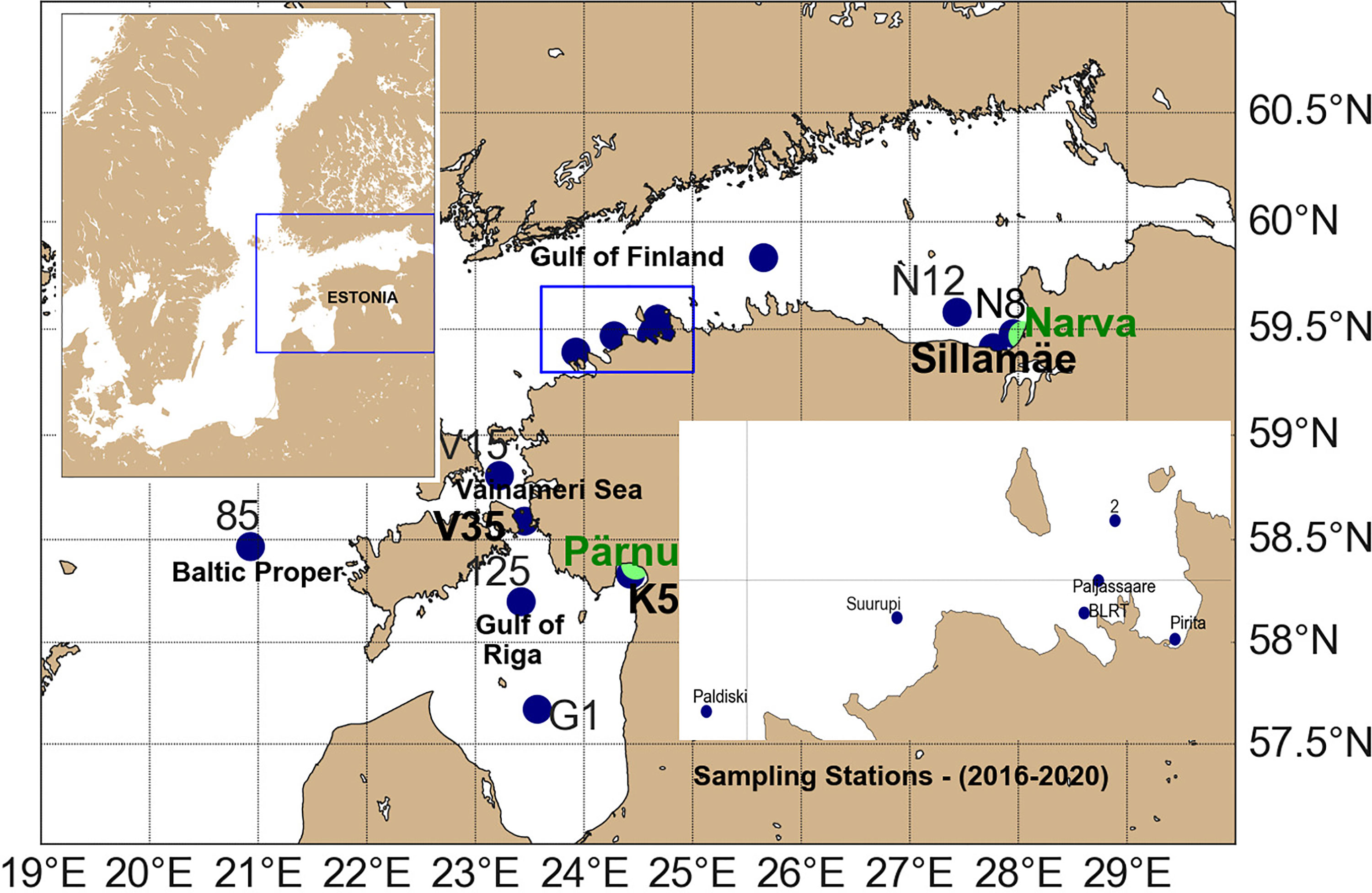
Figure 1 Map of the eastern Baltic Sea with 16 stations of surface water sampling in the BP region (85), GOR (G1, K5, and 125), VS (V15 and V35), GOFW (Paldiski, Suurupi, BLRT, Paljassaare, and Pirita), GOFC (14), and GOFE (N12, Sillamäe, and N8). The locations of Narva and Pärnu river are highlighted in green.

The GOF is an elongated estuarine basin located in the northeastern part of the Baltic Sea with an average depth of 37 m and a maximum depth of 123 m (Leppäranta and Myreberg, 2009). The gulf is about 400 km long, and its width varies between 48 and 135 km (Alenius et al., 1998). There is a free water exchange between the GOF and BP at the western border, and fresh water is discharged mostly to the eastern part of the GOF. The western Estonian coast has two semi-enclosed sub-basins. The GOR covers an area of 140 km from west to east and 150 km from south to north. The surface area of the VS is 2,243 km². The average depth of GOR and VS is 23 m and 4.7 m, respectively. These sub-basins are interconnected and connected with the BP via five straits.

In total, 16 sampling stations were visited in the western Gulf of Finland (GOFW), eastern Gulf of Finland (GOFE), central Gulf of Finland (GOFC), GOR, VS, and northern BP (Figure 1). Stations in the GOFW and GOFE were quite close to shore, while stations in the BP, GOFC, and GOR (excluding Station K5) were offshore. The station network was not the same each year. Visited stations in different years are shown in Table 1. Sampling stations N8 (visited 15 times), 14 (15), Sillamäe (Sill) (14), Paljassaare (Pal) (13), 2 (12), and K5 (11) were sampled more than ten times during the 5-year period. The frequency of sampling times in other stations is as follows: V15 (6), V35 (6), 125 (5), N12 (4), G1 (3), Pirita (Pir) (2), Paldiski (Pald) (1), Suurupi (Suu) (1), and BLRT (1). Please note that station Pal is located close to the largest city wastewater treatment plant outfall in the study area, station N8 close to the Narva river mouth, and station K5 close to the Pärnu river mouth. The detailed observational periods at each sampling site are mentioned in Supplementary Table 1.

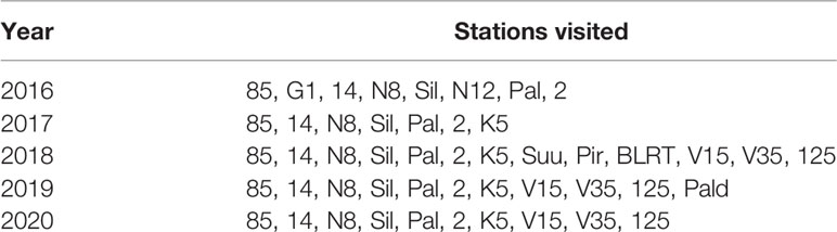
Table 1 MP sampling sites for each year.

MP Sampling and Sample Processing

Surface water samples were collected with a Manta trawl (mesh size 330 µm). The net was deployed 5 m from the side of the ship using a crane and towed at the water surface (not totally submerged) for 15 to 60 min at a speed of approximately 2 knots. The samples were collected in the cod end of the net. The content of the cod end was rinsed with tap water to a metal bucket and sieved through a set of stainless-steel sieves (5,000 µm, 1,000 µm, and 330 µm). Thereafter, particles from each sieve were flushed into a separate glass jar with ultrapure water. Formaldehyde (37%) was added in the proportion of 1 to 100 ml of sample. Samples were kept at room temperature until analysis in the lab.

If the samples contained a lot of organic material, they were left to settle. The solution on top of the settled organic material was pipetted and vacuum filtered onto a 1.6-µm pore size (VWR) glass fiber filter (47 mm diameter). Hydrogen peroxide (34.5%–36.5%) was added to the settled organic material in a proportion of 1:1 and left for oxidation under the ventilation cabinet for up to 7 days. After oxidation, the samples were diluted with ultrapure water and vacuum filtered as described above. The filters were dried in glass Petri dishes in a drying oven (SANYO MOV-212F) at 60°C for 15 min, and the particles remaining on the filters were analyzed using a stereomicroscope (Leica M205 C or Olympus SZX16). All MP particles were counted, partially photographed, and tested with a hot needle to distinguish plastics from other microliter particles (Devriese et al., 2014). The results were calculated by summing the number of MP particles in the analyzed water sample.

In this study, we divided all MP particles into fibers and fragments. The fragments category includes all non-fiber MPs: films, foam, and pellets, and in general, we have identified fibrous plastics. As the MPs monitoring was carried out by the Manta trawl with a mesh size of 330 µm, we categorized them into two size classes (330–999 µm and 1,000–4,999 µm) according to their longest dimension. The water volume was calculated by multiplying the whole area of the trawl mouth with the ship speed and towing time. MP concentration is presented as the number of MP counts per cubic meter (counts/m³). In addition, concentration per square meter (counts/m²) is given in brackets throughout the text.

The 8-color classification scheme by the European Marine Observation and Data Network (EMODnet) was used for color identification that combines similar colors into one group (Galgani et al., 2020). Black/gray, white, blue/green, red/pink/orange/purple, yellow, brown, transparent, and others (golden/silver/multicolor) distinguished from colors.

Reduction of Cross-Contamination

Reduction and monitoring of potential airborne cross-contamination are crucial during sampling, sample processing, and analysis in the laboratory. To detect MP airborne contamination during sampling, samples of plastic-free water were kept in glass jars open on the deck near the sample collection area and later analyzed in the laboratory.

Non-synthetic clothing and cotton lab coats were worn, and glass or metal laboratory supplies were used as much as possible throughout the laboratory analysis. All labware was thoroughly rinsed with ultrapure water before use. Sample processing was done in a ventilation cabinet, except for the filtering through the sieves. Samples were covered with aluminum foil or glass lids from Petri dishes whenever possible.

For the contamination assessment during sample processing in the lab, 100 ml of ultrapure water was filtered through a clean glass fiber filter before each sample processing and analyzed as real samples. Also, one dry blank filter was placed under a ventilation cabinet during filtration and on the table near the stereomicroscope during microscopic analysis. Both blanks were analyzed as samples. In the blank samples, only fibers were found, and blank filter contamination was only a few percentages. Blank samples were used only as a reference. Hence, the overall contamination was less than one plastic fiber per sample on average. The fibers found in the blank samples could be related to airborne contamination from textiles.

Paint flakes were often observed in the samples. All paint flakes data were removed from the dataset for the analysis as their potential sources could not be confirmed.

Statistical Analysis

One-way analysis of variance (ANOVA) was performed to analyze MPs’ spatial and temporal variability. When a substantial difference was discovered, a pairwise comparison using regression test was applied to determine whether the difference was statistically significant. The significance level was set to 5%.

The hourly wind speed components were extracted from ERA-5 (Hersbach, 2020) for seven monitoring stations and bi-linearly interpolated to the exact coordinates using CDO (climate data operators) software (Schulzweida, 2021). Linear regression analysis was used to relate the observed MP abundances to prevailing meteorological conditions (e.g., wind speed). Since the data series were relatively short, as an alternative to linear regression, the conditions during the sampling of lowest and highest MP concentrations were compared.

The sea surface temperature and salinity are taken from the long-term model simulations to understand the hydrophysical conditions during sampling dates. From the model output, two diagnostic parameters are calculated:

a. the lateral gradients of temperature and salinity as |∇_HT| and |∇_HS|

b. the divergence of the current field as u_x+v_y normalized with Coriolis parameter f

Numerical Modeling

The General Estuarine Transport Model (GETM) (Burchard and Bolding, 2002) has been applied to estimate temperature and salinity distributions. GETM is a three-dimensional primitive-equation hydrostatic model with a free surface and built-in vertically adaptive coordinate scheme (Hofmeister et al., 2010), which can significantly reduce numerical mixing in the simulations (Gräwe et al., 2015).

Vertical mixing is calculated using the General Ocean Turbulence Model (GOTM) (Umlauf and Burchard, 2005) using a two-equation k−ϵ model coupled with an algebraic second-moment closure (Canuto et al., 2001; Burchard and Bolding, 2002) to obtain the eddy viscosity and diffusivity. Sub-grid horizontal mixing is parameterized using the Smagorinsky approximation (Smagorinsky, 1963).

The model domain consists of the whole Baltic Sea (Figure 1), and horizontal grid spacing of 0.5 nm (approximately 926 m) is used with 60 vertically adaptive layers. The vertical resolution of the model during simulations is controlled by using the same parameters as in Hofmeister et al. (2010) and Gräwe et al. (2015). Baltic Sea Bathymetry Database (http://data.bshc.pro/, last access: 18 January 2022) with additional data for the GOF from Andrejev et al. (2010) has been used to construct the model bathymetry. The atmospheric forcing (wind stress and surface heat flux components) was calculated from the operational forecast model HIRLAM (High-Resolution Limited Area Model) maintained by the Estonian Weather Service with a spatial resolution of 11 km and a daily forecast interval of 1 h (Männik and Merilain, 2007). The model simulation was performed from April 1, 2010, to December 31, 2020, but the results for 2016 to 2020 have been used in this study.

An open boundary is located at the Danish Straits. Inflow and outflow from the model are calculated using the sea surface height measurements from Gothenburg Station with Flather (1994) radiation. Temperature and salinity at the boundary are relaxed towards climatological profiles by Janssen et al. (1999). Freshwater input from the 54 largest Baltic Sea rivers with basin-wide interannual variability corrected towards values as reported in HELCOM (Johansson and Jalkanen, 2016) has been used. Constant salinity of 0.5 g kg⁻¹ and target cell sea surface temperatures are used for the riverine values.

Initial temperature and salinity fields were taken from the Copernicus reanalysis of the Baltic Sea for the period 1989–2014 (https://doi.org/10.48670/moi-00013, last accessed February 14, 2022). As the product used lower resolutions both in the horizontal and vertical, the thermohaline fields were interpolated to the model grid. The simulation started with sea surface height and current velocities set to zero, i.e., the motionless state, but as previous studies (Lips et al., 2016) have shown, the wind-driven circulation of the Baltic Sea adjusts to forcing within 5 days. More information about the model setup and validation is available from Zhurbas et al. (2018) and Liblik et al. (2020).

Results

MPs were found at all 16 sampling stations. In total, 9,414 MP particles were extracted from 23,199 m³ water of 122 surface water samples. When total MP particles were divided by the total water volume, the mean was 0.41 counts/m³. However, the arithmetic mean of MP concentrations in samples was 0.49 counts/m³ (0.08 counts/m²), and in the regions of BP, GOFC, GOFW, GOFE, GOR, and VS, the mean concentrations were 0.65, 0.59, 0.65, 0.46, 0.33, and 0.11 counts/m³ (0.11, 0.10, 0.11, 0.08, 0.06, and 0.02 counts/m²), respectively. The results show high variability in concentrations (STD ±0.46 counts/m³) and heterogeneity in distribution patterns of MPs in the eastern Baltic Sea. The relative abundance of MP fibers and MP fragments at different sampling sites is presented in Figure 2. The average concentration of MP fibers and MP fragments across the dataset was almost the same: 0.25 and 0.24 counts/m³ (0.04 and 0.04 counts/m²), respectively. The annual mean of the share of fibers was higher in 2016, 2019, and 2020 (Figure 2).

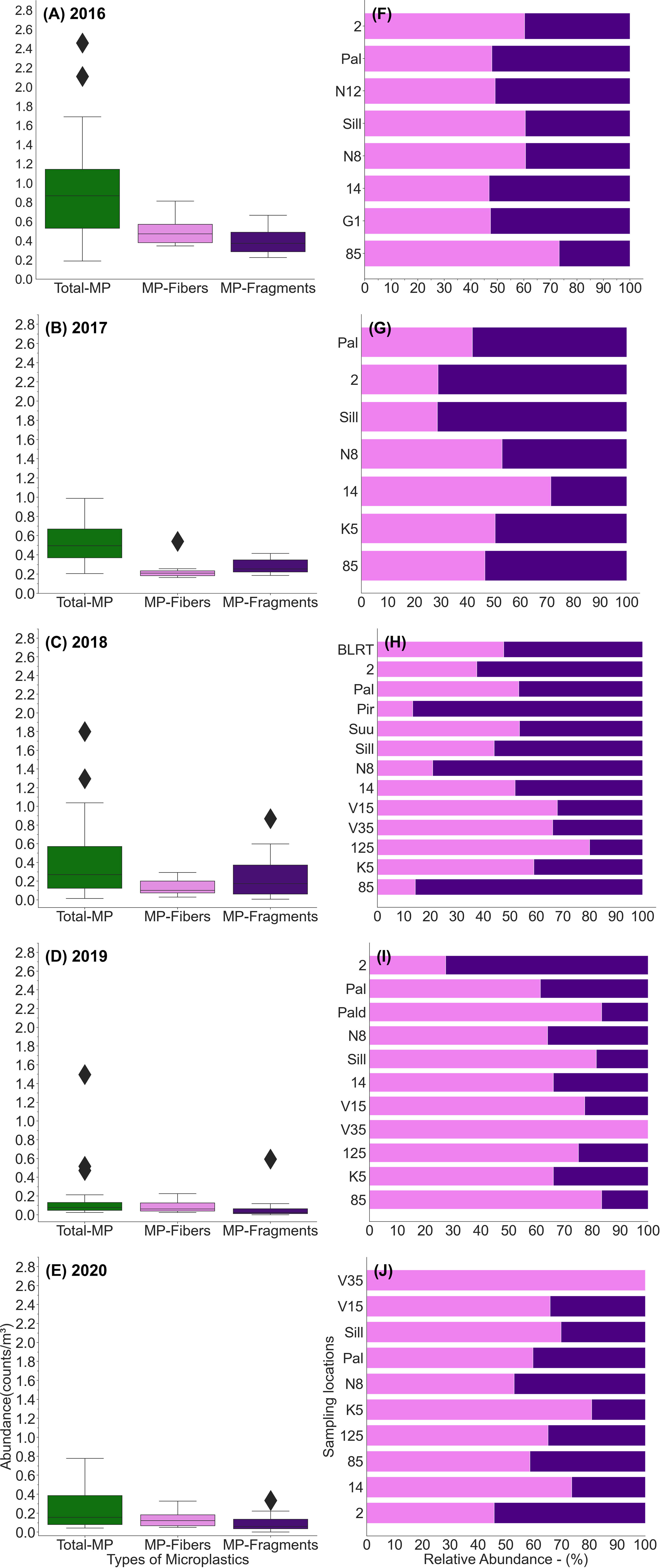
Figure 2 Variability in concentration (A–E) and relative abundance (%) (F–J) of two shapes of MPs at sampling stations in the eastern Baltic Sea.

Spatiotemporal Distribution of Microplastics

Relatively high annual mean MP concentrations (Figure 3; concentrations are shown if the station was visited more than once) were observed in 2016 (Figure 3A). The highest mean concentrations (>1.0 counts/m³) were observed in the GOR (station G1) and the BP (station 85) and at station Pal. Lower values were observed at the GOFE stations. Mean concentrations were in a quite narrow range (0.39–0.58 counts/m³) (0.07–0.1 counts/m²) in the whole area in 2017; only in the GOFC was the value higher (Figure 3B). The highest mean concentration (>1.0 counts/m³) was observed in the BP, while concentrations were 20-fold lower in the GOR and VS in 2018 (Figure 3C). Spatial distribution of the MP concentrations in the GOF had a large range, varying from 0.11 to 0.76 counts/m³ (0.02–0.13 counts/m²) (Figure 3C). Very low mean values (<0.08 counts/m³) were observed in the GOR and VS in 2019 (Figure 3D). Quite low values, except at station 2, were observed in the GOF and BP as well (Figure 3D). A similar pattern was observed in the study area in 2020 (Figure 3E).

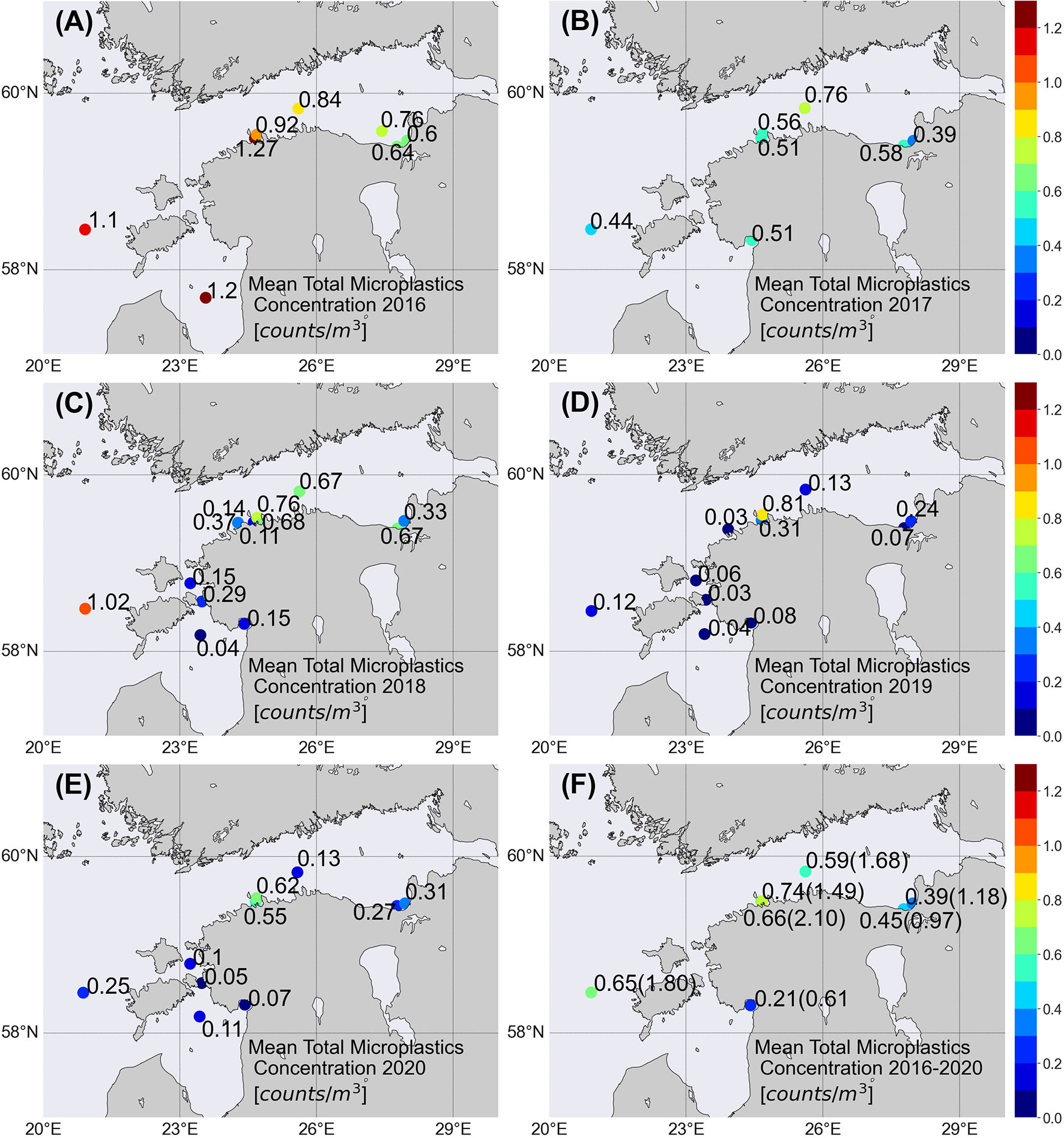
Figure 3 Average MP counts/m³ at each sampling station (A–E). The overall average for 2016–2020 was calculated as an arithmetic mean of all individual concentrations in the sampling location (F). The highest MP concentration (counts/m³) at sampling station is shown in parenthesis (F).

Despite high temporal variability, tendencies in the mean 5-year period spatial pattern can be found (Figure 3F). Significantly higher mean MP, MP fiber, and MP fragment concentrations occurred in the BP and the three areas of GOF compared to the GOR and VS (Figures 4A–C). It is noteworthy that the annual mean concentration in the VS was lower than in the BP in all 3 years (2018–2020) when the VS was sampled (Figures 3C–E). The 5-year mean concentration in the vicinity of Pärnu and Narva river mouths [stations K5 and N8, 0.21 and 0.39 counts/m³ (0.04 and 0.06 counts/m²), respectively] was lower than at the open sea stations (0.59–0.74 counts/m³) (0.10–0.13 counts/m²).

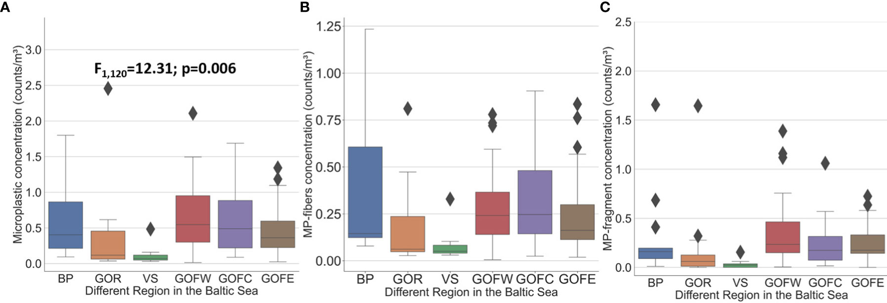
Figure 4 (A) The variability of MP concentrations in different regions of the eastern Baltic Sea in 2016–2020. (B) The variability of MP fiber concentrations in different regions of the eastern Baltic Sea in 2016–2020. (C) The variability of MP fragment concentrations in different regions of the eastern Baltic Sea in 2016-2020.

The maximum concentrations >1.6 counts/m³ were registered at offshore stations in the BP, GOF, GOR, and at station Pal. The highest MP concentration (2.45 counts/m³) (0.43 counts/m²) for the entire study period was recorded at station G1 in the GOR. Maxima were lower (0.6–1.2 counts/m³) at the GOFE stations and near the Pärnu river mouth (station K5). The maximum was only 0.15 counts/m³ (0.03 counts/m²) in the central VS (station V15). However, the latter station was visited only three times.

The mean share of fibers and fragments for the whole area in the 5 years was almost equal (Figure 2). The latter also roughly holds when considering the means of the regions (Figure 5). Thus, the mean spatial distribution of fibers and fragments taken separately (Figures 5A–F and Figures 5G–L) is similar to the total MP concentration (Figure 3F). This means 5-year mean concentrations of fibers and fragments in the vicinity of Pärnu and Narva river mouths are lower than at the open sea stations.

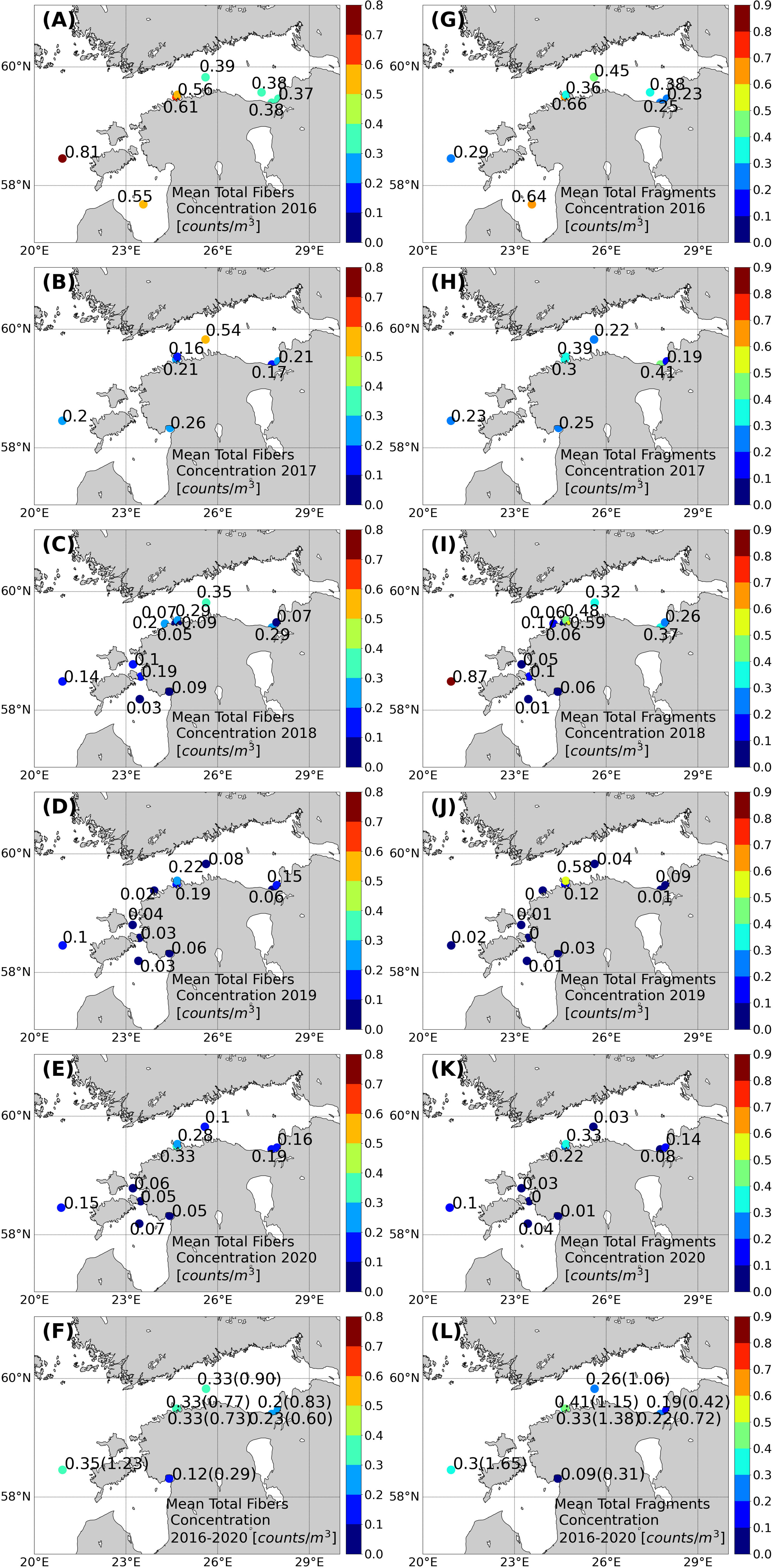
Figure 5 Average MP fiber counts/m³ (A–F) and average MP fragment counts/m³ (G–L) at each sampling station. The overall average for 2016–2020 was calculated as an arithmetic mean of all individual concentrations in the sampling location (F, L). The highest MP fiber and MP fragment concentration (counts/m³) at the sampling station is shown in parentheses (F, L).

The correlation between the concentrations of fibers and fragments in the whole dataset was significant, but rather low (r² = 0.21, p < 0.01, n = 122). Thus, often the spatiotemporal changes of fibers and fragments were not related. However, some of the stations separately revealed quite a strong correlation. High correlation was found at station K5 (r² = 0.87, p < 0.01, n = 11) and Pal (r² = 0.60, p < 0.01, n = 13). Weak but significant correlations were observed at stations 14, Sil, and N8. No correlation was found at stations 2 and 85. For instance, fibers (0.81 counts/m³) (0.14 counts/m²) had the major share at station 85 in the BP in 2016 (Figure 5A). Next year, the concentration of fragments was similar (approximately 0.2–0.3 counts/m³), but the fiber concentration was 0.20 counts/m³ (0.04 counts/m²) (Figure 5B). The share was reversed (compared to 2016) in 2018 when fragments (0.87 counts/m³) (0.15 counts/m²) had the major contribution (Figure 5I). Thus, the highest annual mean concentration of fragments and fibers in the study area was measured in the BP, but in different years. The annual share of fragments higher than 70% occurred only at the coastal stations in the GOF (five occasions) and once at station 85 in the BP. Other stations had a fiber share approximately 50% or higher. The annual mean shares of fragments were lowest in the VS. Note that the total MP concentrations were low there as well.

Microplastics Morphology

The MPs were assorted into eight colors. The most occurred MP color was gray/black (29.7%), followed by white (22.6%) and blue/green (22.4%). Other colors such as red/pink/purple (9.9%), transparent (9.8%), yellow (3.6%), and brown (1.5%) had a lower proportion. Gold-stained plastic was the rarest out of the eight colors, having a percentage share of less than 1%. The maximum share came from white particles when the highest concentrations were detected at stations Pal, 2, 85, and 14. The dominant color for the MP fragments was white and blue/green, and for MP fibers, it was gray/black and blue/green.

Seasonal Variability of Microplastics

The mean concentration in spring and summer was 0.46 counts/m³ (0.08 counts/m²) and 0.36 counts/m³ (0.06 counts/m²), respectively. This tendency of higher concentration in spring compared to summer was revealed at most of the stations (Supplementary Figure 1) except at stations 85, G1, Pir, and V35. The highest seasonal mean concentration (0.81 counts/m³) (0.14 counts/m²) in the study area occurred in the autumn. The mean concentration was higher in autumn than summer at all stations (Supplementary Figure 1). This is reflected in the seasonal pattern across all regions as well (Figure 6). Moreover, the only observations from winter in the GOFC confirm the increasing concentration trend from summer to the cold season. However, due to high variability within each season, the differences between the seasons were statistically not significant. MP fiber concentration differed significantly across all seasons; however, no significant difference was detected for MP fragments. Seasonally, no significant difference was observed between the two size classes—MP (330–999 µm) and MP (1,000–4,999 µm).

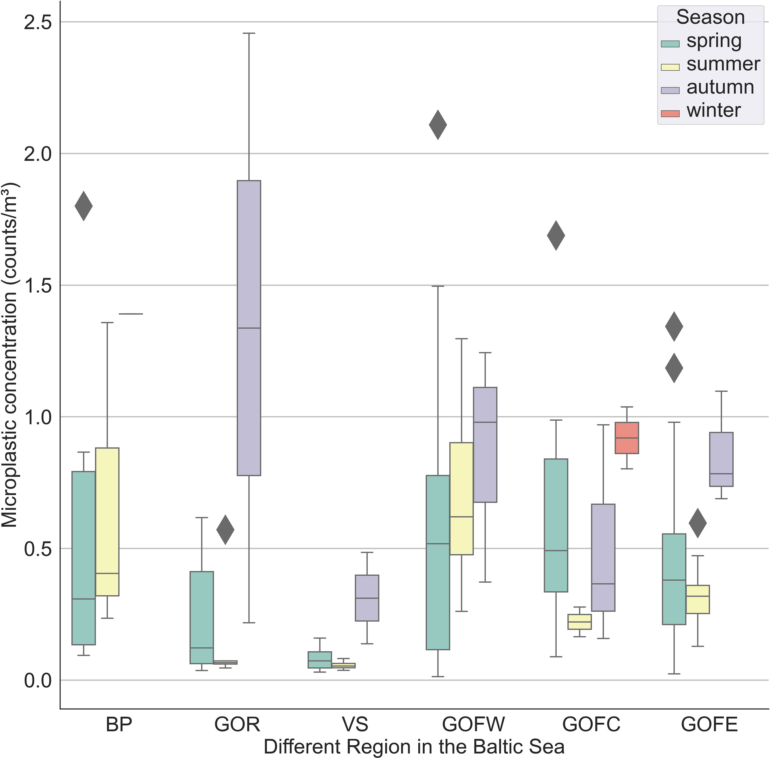
Figure 6 Seasonal variability of MP concentration across different regions in the Baltic Sea.

Impact of Physical Processes on the MP concentration

The impact of physical processes on the MP concentration was studied using the stations with the most consistent observations. Over the 5 years, seven stations had a higher number of samples. We selected two coastal (N8 and K5) and two offshore (14 and 85) stations for further analysis.

The wind is the most obvious physical parameter to affect concentrations on the sea surface, as with increasing wind speed, the particles are mixed deeper. Significant negative correlation between the wind speed and MP concentration was found only at station 14 for MP fragments (r² = 0.35, p = 0.01, n = 15). For the whole dataset and most individual stations, the correlation was low and insignificant. A significant positive relationship between the wind speed and MP abundance was found at the coastal station K5 (r² = 0.47, p = 0.01, n = 11).

At coastal stations K5 and N8, one can assume some effects of freshwater discharge and related MP input due to the vicinity of large rivers. Furthermore, not only the wind speed but also its direction could be critical via influencing convergence/divergence of surface waters. We selected the highest and lowest concentration cases for both stations to compare the effect of the river discharge and wind direction.

At coastal station N8, the highest MP concentrations were detected (1.18 counts/m³) (0.2 counts/m²) when the 3-day mean discharge (589 m³/s) from the Narva river prior to the sampling date was greater than the long-term mean discharge (440 m³/s). Moreover, before the observation of the highest MP concentration, the wind speed and direction at station N8 were favorable for the coastal downwelling (westerly winds with a maximum speed over 8 m/s), which supports the accumulation of MPs along the coast, thus resulting in a high MP concentration (Figure 7A).

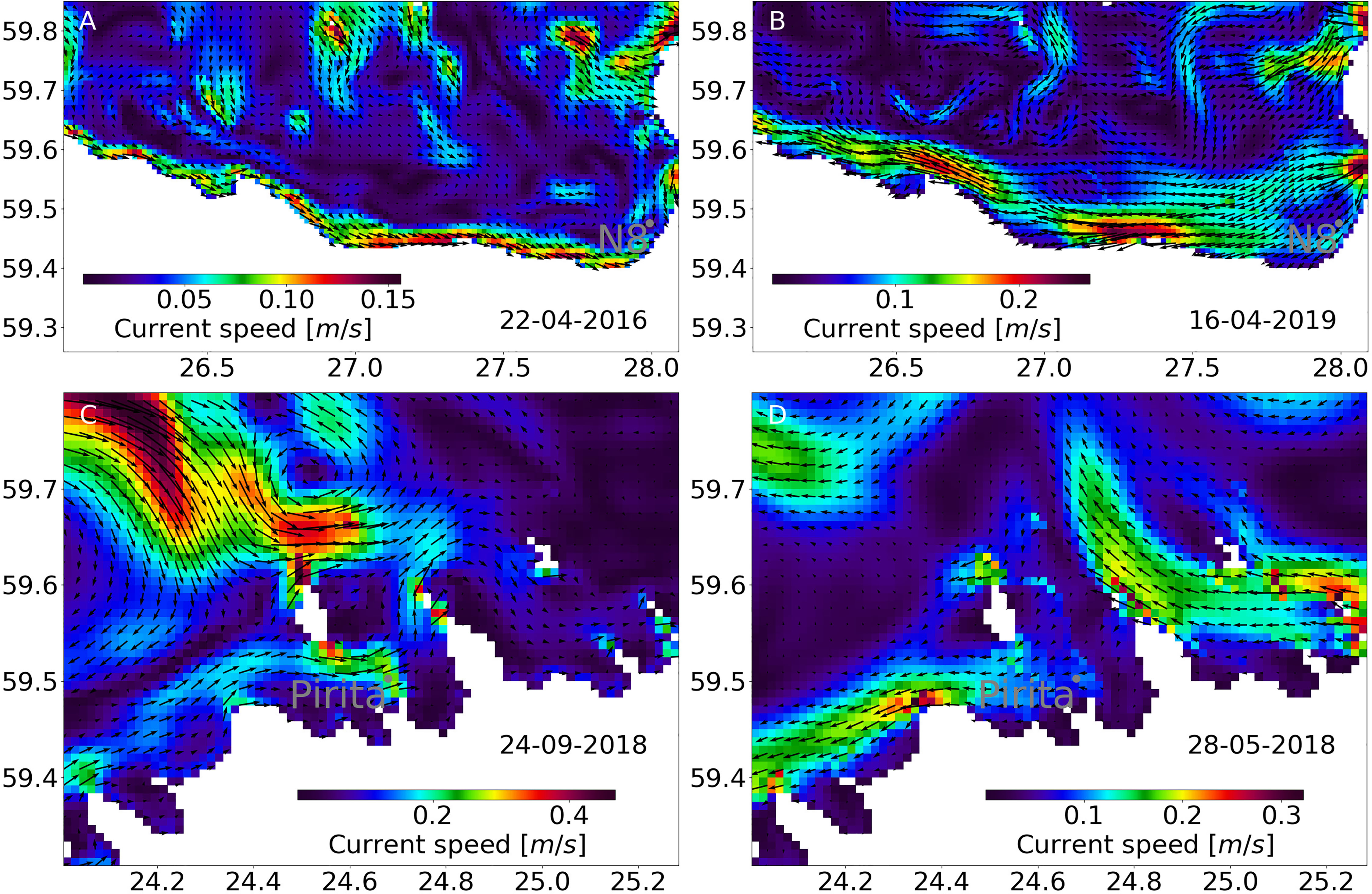
Figure 7 Mean surface current vectors and current speed averaged 3 days before observations of (A) highest concentrations at station N8, (B) lowest concentrations at station N8, (C) highest concentrations at station Pir, and (D) lowest concentrations at station Pir.

In contrast, when the MP concentration was the lowest (0.02 counts/m³) (0.004 counts/m²), the wind conditions before observation indicated the occurrence of coastal upwelling in the area (north easterly winds) (Figure 7B). This water mostly originated from the subsurface, which explains the low MP concentration. Thus, we suggest that variation in coastal mesoscale processes, leading to convergence and divergence of surface waters, could cause both extremely high and low MP.

The impact of coastal upwelling and downwelling events was also visible at the coastal stations in the Tallinn Bay. The highest concentrations at station Pir were measured under the coastal downwelling and the lowest concentrations were measured under the coastal upwelling conditions at the southern coast of the GOF (Figures 7C, D). There is a clear downwelling jet along the coast directed to the east with relatively large current velocities during the high-concentration case (Figure 7C) and an upwelling jet in the opposite direction to the west during the low-concentration case (Figure 7D). Obviously, the large-scale coastal divergence and convergence have a significant impact on the distribution of MPs in the coastal sea.

When comparing the conditions for the lowest and highest MP concentrations at coastal station K5 (depth 5m), strong winds prevailed before the highest MP concentrations were observed. Strong winds cause resuspension of bottom sediments and force MPs to migrate from sediments to the surface, thereby resulting in high MP concentrations at the sea surface. On the other hand, weakened wind-induced resuspension leads to lower MP concentrations at the sea surface in shallow areas.

In order to better understand the hydrodynamic conditions in the offshore stations 85 and 14, we looked at the simulated sea surface temperature and salinity fields in the vicinity of the stations along with the convergence and divergence based on the modeled current components during dates with the observed highest and lowest MP values (Figure 8). The statistical parameters of different fields are summarized in Table 2.

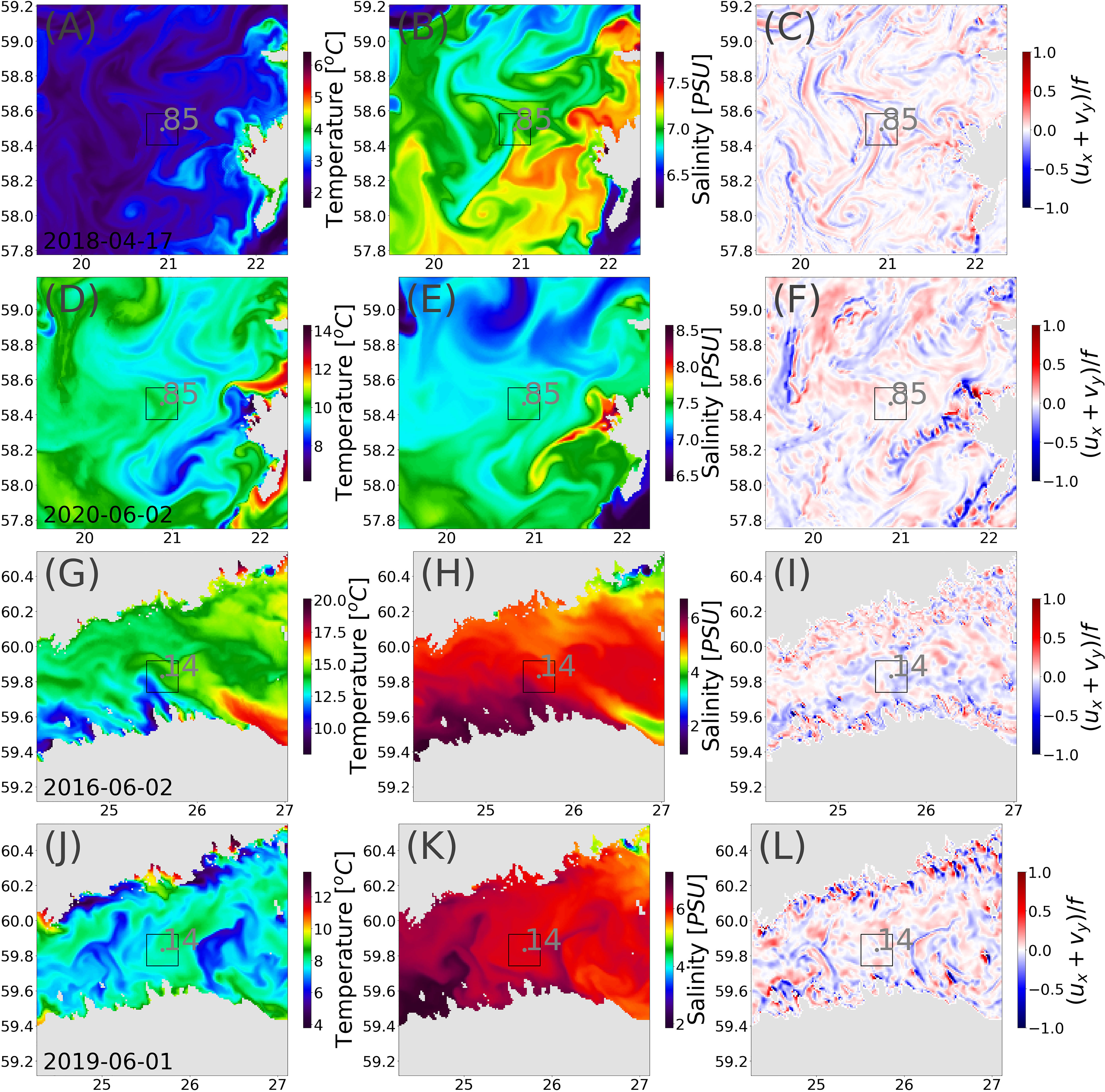
Figure 8 Snapshots of surface temperature (A, D, G, J), surface salinity (B, E, H, K), and current field divergence, u_x+v_y/f, in the surface layers (C, F, I, L) during the highest and lowest measured concentration of MPs at selected stations. The gray box indicates the location around measurement location with 10-km distance.

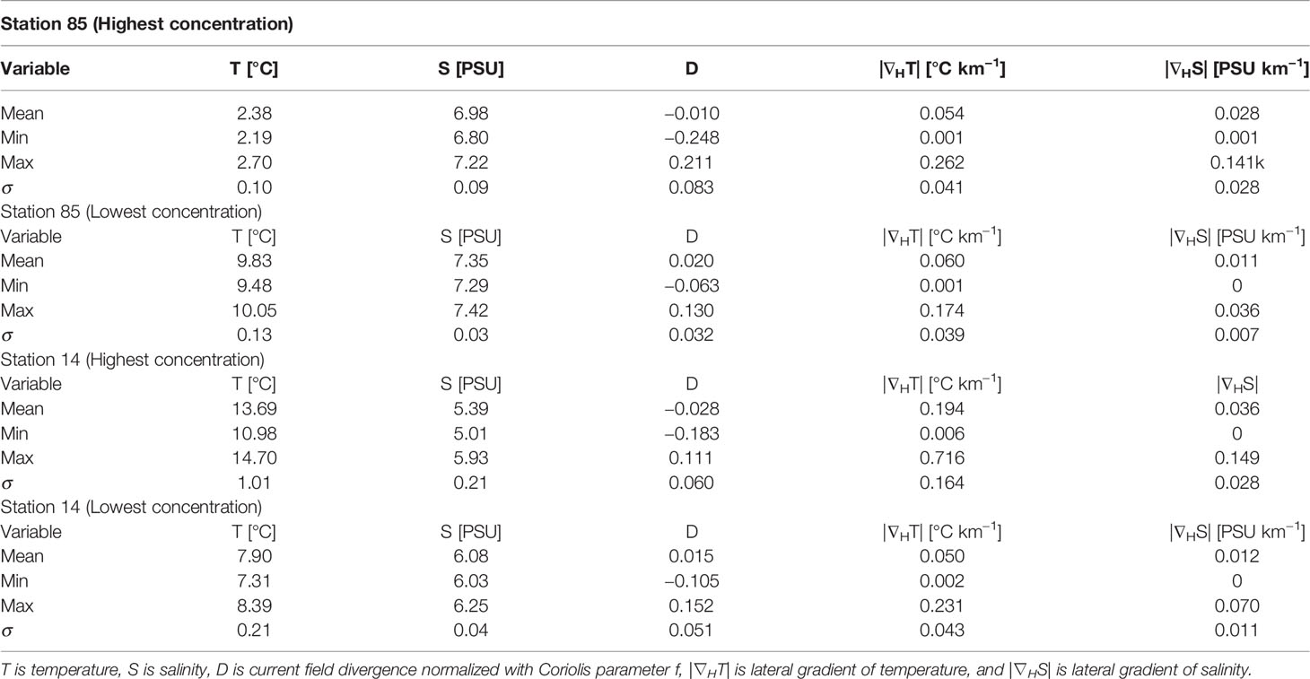
Table 2 Statistical values of different surface parameters around the monitoring stations during the observed highest and lowest value of MPs.

In the high-concentration cases at both stations, strong lateral gradients in the salinity and temperature fields in the vicinity of the stations are seen (Figures 8G, H). During low-concentration cases, the lateral gradients are much weaker, and the variance of the fields is much smaller. In addition, the divergence during the high-concentration case was mostly negative, suggesting convergence, i.e., accumulation of the matter in the surface layer. During the low-concentration case, the divergence was mostly positive in the vicinity of the station.

Although the mean temperature and range during the high-concentration case was smaller than during the low-concentration case at 85, the range and variability of salinity was at least two times larger (Table 2). The variability of the salinity gradient around the station was almost 6 times larger. At station 14, the variance (shown as standard deviation in Table 2) of all parameters are greater during the high-concentration case.

Discussion

We have reported results from the 5-year MP observations in the eastern Baltic Sea. Next, we compare our findings with previous studies that collected data using surface trawling (Manta trawl) like us in the Baltic and global oceans. In the sea surface layer of the Baltic Sea, Aigars et al. (2021) detected an MP concentration of 0.09–4.43 counts/m³, Karlsson et al. (2020) found 0.18–0.92 counts/m³ in the Gullmar fjord at the Swedish west coast, 0.05–0.09 counts/m³ were observed in the South Funen Archipelago (Tamminga et al., 2018), Gewert et al. (2017) measured 0.19–7.73 counts/m³ in the Stockholm Archipelago, and 0–0.8 counts/m³ were found in the GOF (Setälä et al., 2016). In the Arctic waters, Lusher et al. (2015) revealed MP concentrations of 0–1.31 counts/m³, 0.07–9.25 counts/m³ were measured in the Eastern Mediterranean Sea (Adamopoulou et al., 2021), 1.82 counts/m³ were observed in the Mediterranean Sea (Zeri et al., 2018), and 0.06–25.9 counts/m³ were found in the Eastern Indian Ocean (Li et al., 2021).

Although Aigars et al. (2021) collected samples at numerous stations during 1 year, while we conducted measurements at three stations, during 5 years, the mean concentrations in the central GOR were roughly in the same order. Our observations revealed lower concentrations in the northern GOR and the Pärnu Bay; however. Setälä et al. (2016) identified an average MP concentration of 0.3 counts/m³ in the GOFC region, and our investigation revealed 0.59 counts/m³. We can conclude that the concentrations registered in our study—in the range of 0.01 to 2.45 counts/m³ (0.002–0.43 counts/m²) with a mean concentration of 0.49 counts/m³ (0.08 counts/m²)—are in the same order as previous studies in the Baltic Sea.

The mean concentrations in the three subregions in the GOF were in the range of 0.46–0.65 counts/m³, while it was 0.33 counts/m³ in the GOR. The difference between concentrations in the GOR and GOF could be explained by human pressure. Population in the catchment area per surface area of the GOF is ca. 400 inhabitants km⁻² while it is 150 inhabitants km⁻² in the GOR catchment (HELCOM, 2004). Note that in the easternmost part of the GOF, in the area we did not cover, the MP concentrations are probably higher than we observed due to the impact of river Neva (Martyanov et al., 2021). If we combine our results with Aigars et al. (2021), a meridional pattern is revealed in the GOR: higher MP concentrations in the south and lower MP concentrations in the north. This could be related to the population in the catchment areas as well. The water entering the southern part of the GOR is impacted by ca. 2.4 million inhabitants while the total population in the catchment area of the GOR is ca. 2.7 million.

The low human pressure is a likely reason behind the small mean concentration in the VS. The catchment area of the VS has an extremely low population, and there are no larger towns or other considerable point sources at the coast of the VS. Low MP concentrations in a similar area, in the South Funen Archipelago in Denmark, were explained by the sheltered position of the study area, low human pressure on adjacent islands, and the absence of any major potential point sources (Tamminga et al., 2018).

We registered considerable amounts of MPs at stations Pal (2.10 counts/m³) and 2 (1.49 counts/m³) in proximity to the city of Tallinn. Our observations follow previous studies that reported that the MP particle concentrations are frequently greater near densely populated urban areas with pollution sources such as industry and wastewater treatment plants (Yonkos et al., 2014; Gewert et al., 2017; Schönlau et al., 2020).

High mean MP concentration was detected at offshore station 85. This is a somewhat controversial result as earlier studies have reported higher values near coasts and rather low values offshore in the BP (e.g., Aigars et al., 2021). No major rivers enter the area, or remarkable point sources (cities and towns) are nearby. On the one hand, a possible explanation could be that the northern BP is the accumulation zone, where the discharge and buoyant particles from different basins (the GOF, GOR, Bothnian region, and south- and eastern BP) are concentrated. Secondly, the mean cyclonic current structure of the BP (Placke et al., 2018; Liblik et al., 2022) recirculates/traps the surface water in the basin for a longer period. In addition, MPs exhibit different buoyancy characteristics based on their density, shape, size, and biofouling rate (Adamopoulou et al., 2021). Convergence and downwelling act as a sorting mechanism, with relatively larger particles staying in the surface layers and smaller particles getting transported deeper in the water column (van Sebille et al., 2020). The biofilm growth is generally faster for smaller particles due to their high surface-to-volume ratios (Tsiaras et al., 2021). Thus, the buoyancy patterns described above and the fact that nearly 81% of MPs detected were smaller than 1 mm allow us to justify the high mean MP concentration at station 85. Recently, it has been shown that the region is prone to be affected by the submeso- and mesoscale activity (Väli and Zhurbas, 2021; Zhurbas et al., 2022), which can contribute to the convergence and divergence of MPs in the surface layers. We showed that high variability and convergence at the (sub)mesoscale could be a factor leading to high MP concentrations, but further investigations are needed to understand the pathways and reasons behind the phenomenon.

We considered two shapes of the MP particles in the current study: fibers and fragments, which accounted for 96% of the encountered particles in the eastern Baltic according to the recent study (Aigars et al., 2021). MP fragments are more likely to break up into smaller pieces and are caught in the Manta trawl than other MPs (Li et al., 2021). Synthetic fibers derived from textile materials could enter the aquatic ecosystem through sewage systems, surface runoff, or atmospheric transport and deposition (Bai et al., 2018; Liu et al., 2019; Wang et al., 2020).

The share of fibers (51%) and fragments (49%) was approximately equal in the current study. The latter is valid for the whole dataset, as well as the subregions. However, the share of shapes and concentrations might be influenced by the sampling method: Manta trawling with the mesh size of 330 µm. Many studies reported more fibers on the sea surface (Setälä et al., 2016; Bagaev et al., 2017; Gewert et al., 2017; Tamminga et al., 2018; Aigars et al., 2021), compared with fragments. On the other hand, some studies showed a lower proportion of fibers (Zhang et al., 2017; Pan et al., 2019; Karlsson et al., 2020). When samples are collected using the Manta trawl, MP fibers might leak in high numbers through the 330-µm mesh but could be more efficiently trapped when the mesh size is smaller (<100 µm; Setälä et al., 2016). However, even when a smaller mesh size (100 µm) is used, the number of fibers does not appear to rise, as fiber size, particularly from clothes, is less than 20 µm (Setälä et al., 2016).

Despite the equal share of fibers and fragments, the correlation between the concentration of the two shapes in the whole dataset was weak, although significant. However, high correlations were found near the Pärnu river mouth at station K5 (r² = 0.87) and near the outlet of the Paljassaare wastewater treatment plant, at station Pal (r² = 0.60). In the rest of the stations, there was a significant weak correlation, except at station 2 in the GOF and offshore station 85 in the BP, where the correlation was not found. Due to disturbance-induced vertical transport, small size MPs get resuspended to the surface layer (Xia et al., 2021). As K5 is a shallow station (depth, 5 m), and nearly three-fourths of MP detected are small, we suggest that the high correlation is related to the resuspension of MP to the sea surface layer. Correlation further off the sources was weaker due to the impact of marine processes, e.g., biofouling and vertical mixing, which could have a different effect on the fibers and fragments.

The MP fragments were mostly white, blue/green, and gray/black, whereas MP fibers were mostly gray/black and blue/green in the current study. This result is consistent with other studies where MP fragments and MP fibers were reported (Zhang et al., 2017; Karlsson et al., 2020; Aigars et al., 2021). The share between the two size classes 330–999 µm and 1,000–4,999 µm was 75% and 25%, respectively. The higher number of particles with decreasing size has been documented earlier in the eastern Baltic Sea (Setälä et al., 2016; Aigars et al., 2021).

The mean concentration was higher in autumn than in summer in all regions and stations. This seasonal signal is likely related to the biofouling and consequent sinking of the MP (Kaiser et al., 2017). Spring and summer are biologically active seasons in the Baltic Sea (Lips et al., 2014; Kahru et al., 2016; Purina et al., 2018). Decay and deepening of the seasonal thermocline and cooling of the upper mixed layer water start in the second half of August in the eastern Baltic Sea (Liblik and Lips, 2011; Skudra and Lips, 2017), which leads to the decrease of organic matter production (e.g., Gasiūnaitė et al., 2005), reduced biofouling, and consequently declined sinking rate of the MP. Moreover, the density of the upper mixed layer increases in autumn, which increases the buoyancy of the MP and reduces the sinking probability as well.

The shorter-term and smaller-scale spatial variability of the MP concentration in the sea surface is shaped by various processes such as advection, divergence, convergence, and vertical mixing (Auta et al., 2017; Lebreton et al., 2018; Zhang et al., 2020). The wind mixing distributes the MP vertically (Kukulka et al., 2012); thus, the MP concentration in the surface layer and wind speed can be negatively correlated (e.g., Schönlau et al., 2020). We found a significant negative, but weak correlation between the wind speed and the MP concentration only at offshore station 14.

The highest concentrations of the MP at the coast of Narva Bay were observed during the downwelling event while the lowest value was detected during the coastal upwelling event. There was a 60-fold difference between the highest and lowest case. The low values during upwelling can be explained by the subsurface origin of the water. The upwelling water originates from the cold intermediate layer in the GOF (Lips et al., 2009). The downwelling causes convergence of the upper layer water and the upper mixed layer in summer could deepen over 40 m (Liblik et al., 2017). Despite the downward movement, the buoyant-enough particles tend to stay at the surface and accumulate (Kooi et al., 2016; Waldschläger and Schüttrumpf, 2019). Thus, in the enclosed sea, where wind from any direction causes downwelling/upwelling along some coastal sections (Myrberg and Andrejev, 2003), the coastal mesoscale processes can potentially cause remarkable variability in the MP concentrations. Moreover, mesoscale eddies could redistribute the MP. The anticyclonic eddies converge the debris, and thus, concentrations there can be much higher compared to cyclonic eddies as shown in other areas (Brach et al., 2018). It is probable that the submesoscale processes, which are evident in the observations (e.g., Lips et al., 2016) and which converge and diverge tracers according to simulations (e.g., Zhurbas et al., 2022) in the smaller spatiotemporal scale, affect the MP concentrations and pathways as well in the Baltic Sea. Our samples were collected along a 1- to 4-km long line; thus, to study the MP in the submesoscale in more detail, other measurement methods, e.g., in situ pumping (Karlsson et al., 2020), should be implemented.

Conclusions

The dataset analyzed in the present study provides the first view on MP pollution and its spatiotemporal variability in the surface water of the eastern Baltic Sea. MPs were found in all 122 samples, and their concentration varied from 0.01 to 2.45 counts/m³ with a mean concentration of 0.49 counts/m³. The obtained concentration ranges, the share of the MP fragments and fibers, and the color composition of MPs generally agree with previous studies in the neighboring areas. The regional differences in the mean MP concentrations in the GOF, GOR, and Väinameri Archipelago Sea are likely related to the human pressure (population) in the catchment areas. The seasonal increase in the concentration from summer to autumn can likely be explained by the decline in the biofouling in autumn and related decrease in the sinking rate of particles.

The high variability in the observations was probably the result of multiple processes, which could not be fully captured by the design of the monitoring program. However, we managed to show that upwellings and downwellings, and wind mixing play a role in the variability of the sea surface MP concentration. It is likely that other (sub)mesoscale processes alter the MP concentrations in the surface layer as well. To improve the knowledge on the pathways of the MPs, the processes in the (sub)mesoscale from the sources to offshore should be addressed by further dedicated observational and modeling studies. Likewise, the measurement and modeling effort to estimate the land–sea and water column–sediment fluxes of MPs should be sought.

Data Availability Statement

The raw data supporting the conclusions of this article will be made available by the authors, without undue reservation. The whole dataset is available via EMODnet Chemistry and Estonian Environmental Database (KESE).

Author Contributions

AM: Conceptualization, Data curation, Formal analysis, Methodology, Validation, Software, Visualization, and Writing—original draft. NB and KL: Methodology, Data curation, Writing—original draft, and Resources. IL: Conceptualization, Resources, Validation, Writing—review and editing. TL: Conceptualization, Data curation, Visualization, Validation, and Writing—review and editing. GV: Conceptualization, Data curation, Validation, Software, Visualization, and Writing—review and editing. UL: Conceptualization, Methodology, Formal analysis, Visualization, Validation, and Writing—review and editing. All authors contributed to the article and approved the submitted version.

Funding

Microplastics monitoring was financed by the Estonian Ministry of the Environment, Environmental Agency and Environmental Investment Center. This work was supported by the Estonian Research Council grant PRG602, H2020 project CLAIM (grant agreement no. 774586), and JPI Oceans projects ANDROMEDA (agreement no 4-1/20/160) and RESPONSE (agreement no 4-1/20/161).

Conflict of Interest

The authors declare that the research was conducted in the absence of any commercial or financial relationships that could be construed as a potential conflict of interest.

Publisher’s Note

All claims expressed in this article are solely those of the authors and do not necessarily represent those of their affiliated organizations, or those of the publisher, the editors and the reviewers. Any product that may be evaluated in this article, or claim that may be made by its manufacturer, is not guaranteed or endorsed by the publisher.

Acknowledgments

Allocation of computing time from HPC at Tallinn University of Technology and University of Tartu is gratefully acknowledged. The GETM community at Leibniz Institute of Baltic Sea research (IOW, Warnemünde) is acknowledged for the code maintenance and support.

Supplementary Material

The Supplementary Material for this article can be found online at: https://www.frontiersin.org/articles/10.3389/fmars.2022.875984/full#supplementary-material

References

Adamopoulou A., Zeri C., Garaventa F., Gambardella C., Loakeimidis C., Pitta E. (2021). Distribution Patterns of Floating Microplastics in Open and Coastal Waters of the Eastern Mediterranean Sea (Ionian, Aegean, and Levantine Seas). Front. Mar. Sci. 8. doi: 10.3389/fmars.2021.699000. ISSN 2296-7445.
Aigars J., Barone M., Suhareva N., Putna-Nimane I., Dimante-Deimantovica I. (2021). Occurrence and Spatial Distribution of Microplastics in the Surface Waters of the Baltic Sea and the Gulf of Riga. Mar. Pollut. Bull. 172, 1–10. doi: 10.1016/j.marpolbul.2021.112860
Alenius P., Myrberg K., Nekrasov A. (1998). The Physical Oceanography of the Gulf of Finland: A Review. Boreal Environ. Res. 3, 97–125.
Andrady A. L. (2011). Microplastics in the Marine Environment. Mar. Pollut. Bull. 62, 1596–1605. doi: 10.1016/j.marpolbul.2011.05.030. ISSN 0025-326X.
Andrejev O., Sokolov A., Soomere T., Värv R., Viikmäe B. (2010). The Use of High-Resolution Bathymetry for Circulation Modelling in the Gulf of Finland. Est. J. Eng. 16 (3), 187. doi: 10.3176/eng.2010.3.01
Arthur C., Baker J., Bamford H. (2009). Proceedings of the International Research Workshop on the Occurrence, Effects, and Fate of Microplastic Marine Debris. National Oceanic and Atmospheric Administration Technical Memorandum Nos-or&R-30. Silver Spring, MD, USA: NOAA Marine Debris Division.
Auta H. S., Emenike C. U., Fauziah S. H. (2017). Distribution and Importance of Microplastics in the Marine Environment: A Review of the Sources, Fate, Effects, and Potential Solutions. Environ. Int. 102, 165–176. doi: 10.1016/j.envint.2017.02.013
Bagaev A., Mizyuk A., Khatmullina L., Isachenko I., Chubarenko I. (2017). Anthropogenic Fibers in the Baltic Sea Water Column: Field Data, Laboratory and Numerical Testing of Their Motion. Sci. Total Environ. 599–600, 560–571. doi: 10.1016/j.scitotenv.2017.04.185. ISSN 0048-9697.
Bai M., Zhu L., An L., Peng G., Li D. (2018). Estimation and Prediction of Plastic Waste Annual Input Into the Sea From China. Acta Oceanol. Sin. 37, 26–39. doi: 10.1007/s13131-018-1279-0
Boucher J., Friot D. (2017). Primary Microplastics in the Oceans: A Global Evaluation of Sources. Gland, Switzerland: IUCN. doi: 10.2305/IUCN.CH.2017.01.en
Brach L., Deixonne P., Bernard M. F., Durand E., Desjean M. C., Perez E., et al. (2018). Anticyclonic Eddies Increase Accumulation of Microplastic in the North Atlantic Subtropical Gyre. Mar. Pollut. Bull. 126, 191–196. doi: 10.1016/j.marpolbul.2017.10.077
Burchard H., Bolding K. (2002). Getm – A General Estuarine Transport Model. Scientific Documentation. Tech Rep EUR 20253 En (Ispra: press. Copernicus Marine Service). Available at: https://resources.marine.copernicus.eu/products.
Canuto V. M., Howard A., Cheng Y., Dubovikov M. S. (2001). Ocean Turbulence. Part I: One-point Closure Model—Momentum and Heat Vertical Diffusivities. J. Phys. Oceanography 31 (6), 1413–1426. doi: 10.1175/1520-0485(2001)031<1413:OTPIOP>2.0.CO;2
Cole M., Lindeque P., Halsband C., Galloway T. S. (2011). Microplastics as Contaminants in the Marine Environment: A Review. Mar. Pollution Bull. 62 (12), 2588–2597. doi: 10.1016/j.marpolbul.2011.09.025. ISSN 0025-326X.
Collignon A., Hecq J. H., Galgani F., Collard F., Goffart A. (2014). Annual Variation in Neustonic Micro- and Meso-Plastic Particles and Zooplankton in the Bay of Calvi (Mediterranean-Corsica). Mar. Pollut. Bull. 79 (1-2), 293–298. doi: 10.1016/j.marpolbul.2013.11.023
Devriese L., De Witte B., Bekaert K., Hoffman S., Vandermeersch G., Cooreman K., et al. (2014). Quality Assessment of the Blue Mussel (Mytilusedulis): Comparison Between Commercial and Wild Types. Mar. Pollut. Bull. 85 (1), 146–155. doi: 10.1016/j.marpolbul.2014.06.006
Eriksen M., Mason S., Wilson S., Box C., Zellers A., Edwards W., et al. (2013). Microplastic Pollution in the Surface Waters of the Laurentian Great Lakes. Mar. Pollut. Bull. 77 (1-2), 177–182. doi: 10.1016/j.marpolbul.2013.10.007
Flather R. A. (1994). A Storm Surge Prediction Model for the Northern Bay of Bengal With Application to the Cyclone Disaster in April 1991. J. Phys. Oceanography 24 (1), 172–190. doi: 10.1175/1520-0485(1994)024<0172:ASSPMF>2.0.CO;2
Gago J., Portela S., Filgueiras A. V., Salinas M. P., Macías D. (2019). Ingestion of Plastic Debris (Macro and Micro) by Longnose Lancetfish (Alepisaurus Ferox) in the North Atlantic Ocean Reg. Stud. Mar. Sci. 33, 100977. doi: 10.1016/j.rsma.2019.100977
Galgani F., Giorgetti A., Vinci M., Moigne M., Moncoiffe G., Brosich A., et al. (2020). Proposal for Gathering and Managing Data Sets on Marine Micro-Litter on a European Scale. (Belgium: EMODnet Oostende). 34 pp. doi: 10.6092/8ce4e8b7-f42c-4683-9ece-c32559606dbd
Gasiūnaitė Z. R., Cardoso A., Heiskanen A., Henriksen P., Kauppila P., Olenina I., et al. (2005). Seasonality of Coastal Phytoplankton in the Baltic Sea: Influence of Salinity and Eutrophication. Estuarine Coastal Shelf Sci. 65, 239–252. doi: 10.1016/j.ecss.2005.05.018
GESAMP (2019). Guidelines on the Monitoring and Assessment of Plastic Litter and Microplastics in the Ocean. GESAMP Rep. Stud. Ser. 99, 130.
Gewert B., Ogonowskia M., Barth A., MacLeoda M. (2017). Abundance and Composition of Near Surface Microplastics and Plastic Debris in the Stockholm Archipelago, Baltic Sea. Mar. Pollut. Bull. 120, 292–302. doi: 10.1016/j.marpolbul.2017.04.062
Gräwe U., Naumann M., Mohrholz V., Burchard H. (2015). Anatomizing One of the Largest Saltwater Inflows Into the Baltic Sea in December 2014. J. Geophys Res. Ocean 120 (11), 7676–7697. doi: 10.1002/2015JC011269
He P., Chen L., Shao L., Zhang H., Lü F. (2019). Municipal Solid Waste (MSW) Landfill: A Source of Microplastics? -Evidence of Microplastics in Landfill Leachate, Water Research, Vol. Volume 159. Pages 38–45 ELSEVIER. doi: 10.1016/j.watres.2019.04.060
HELCOM (2004). The Fourth Baltic Sea Pollution Load Compilation (Plc-4). Baltic Sea Environ. Proc. No 93, 1–189.
Hersbach H. (2020). The ERA5 Global Reanalysis. Q. J. R. Meteorol. Soc. 146.730, 1999–2049. doi: 10.1002/qj.3803
Hidalgo-Ruz V., Gutow L., Thompson R. C., Thiel M. (2012). Microplastics in the Marine Environment: A Review of the Methods Used for Identification and Quantification. Environ. Sci. Technol. 46 (2012) pp, 3060–3075. doi: 10.1021/es2031505
Hofmeister R., Burchard H., Beckers J. M. (2010). Non-Uniform Adaptive Vertical Grids for 3D Numerical Ocean Models, Ocean Modelling, Vol. Volume 33. ELSEVIER. doi: 10.1016/j.ocemod.2009.12.003
Jambeck J. R., Geyer R., Wilcox C., Siegler T. R., Perryman M., Andrady A., et al. (2015). Marine Pollution. Plast. Waste Inputs Land. Into Ocean Sci. 347, 768–771. doi: 10.1126/science.1260352
Janssen F., Schrum C., Backhaus J. O. (1999). A Climatological Data Set of Temperature and Salinity for the Baltic Sea and the North Sea. Dtsch. Hydrogr. Z. 51 (S9), 5–245. doi: 10.1007/BF02933676
Johansson L., Jalkanen J. P. (2016). Emissions From Baltic Sea Shipping in 2015 (HELCOM: Baltic Sea Environment Fact Sheets).
Kahru M., Elmgren R., Savchuk O. P. (2016). Changing Seasonality of the Baltic Sea. Biogeosciences 13, 1009–1018. doi: 10.5194/bg-13-1009-2016
Kaiser D., Kowalski N., Waniek J. J. (2017). Effects of Biofouling on the Sinking Behavior of Microplastics. Environ. Res. Lett. 12, 1–12. doi: 10.1088/1748-9326/aa8e8b
Karlsson T. M., Kärrman A., Rotander A., Hassellöv M. (2020). Comparison Between Manta Trawl and In Situ Pump Filtration Methods, and Guidance for Visual Identification of Microplastics in Surface Waters. Environ. Sci. Pollut. Res. 27, 5559–5571. doi: 10.1007/s11356-019-07274-5
Kooi M., Reisser J., Slat B., Ferrari F., Schmid M., Cunsolo S., et al. (2016). The Effect of Particle Properties on the Depth Profile of Buoyant Plastics in the Ocean. Sci. Rep. 6, 1–10. doi: 10.1038/srep33882
Kukulka T., Proskurowski G., Morét S., Meyer D., Law K. (2012). The Effect of Wind Mixing on the Vertical Distribution of Buoyant Plastic Debris. Geophysical Res. Lett. 39, L07601. doi: 10.1029/2012GL051116
Lebreton L., Slat B., Ferrari F. (2018). Evidence That the Great Pacific Garbage Patch Is Rapidly Accumulating Plastic. Sci. Rep. 8, 4666. doi: 10.1038/s41598-018-22939-w
Leppäranta M., Myreberg K. (2009). Physical Oceanography of the Baltic Sea (Berlin, Heidelberg: Springer Berlin Heidelberg). doi: 10.1007/978-3-540-79703-6
Liblik T., Lips U. (2011). Characteristics and Variability of the Vertical Thermohaline Structure in the Gulf of Finland in Summer. Boreal Environ. Res. 16, 73–83.
Liblik, Taavi, Lips, Urmas (2017). Variability of Pycnoclines in a Three-Layer, Large Estuary: The Gulf of Finland. Boreal Environ. Res. 22, 27–47.
Liblik T., Väli G., Lips I., Lilover M. J., Kikas V., Laanemets J. (2020). The Winter Stratification Phenomenon and Its Consequences in the Gulf of Finland, Baltic Sea. Ocean Sci. 16, 1475–1490. doi: 10.5194/os-16-1475-2020
Liblik T., Väli G., Salm K., Laanemets J., Lilover M.-J., Lips U. (2022). Quasi-Steady Circulation Regimes in the Baltic Sea. Ocean Sci. Discuss. doi: 10.5194/os-2021-123
Lips U., Kikas V., Liblik T., Lips I. (2016). Multi-Sensor in Situ Observations to Resolve the Sub-Mesoscale Features in the Stratified Gulf of Finland, Baltic Sea. Ocean Sci. 12, 715–732. doi: 10.5194/os-12-715-2016
Lips I., Lips U., Liblik T. (2009). Consequences of Coastal Upwelling Events on Physical and Chemical Patterns in the Central Gulf of Finland (Baltic Sea). Continental Shelf Res. 29, 1836–1847. doi: 10.1016/j.csr.2009.06.010
Lips I., Rünk N., Kikas V., Meerits A., Lips U. (2014). High-Resolution Dynamics of the Spring Bloom in the Gulf of Finland of the Baltic Sea. J. Mar. Syst. 129, 135–149, 129. doi: 10.1016/j.jmarsys.2013.06.002. ISSN 0924-7963.
Lips U., Zhurbas V., Skudra M., Väli G. (2016). A Numerical Study of Circulation in the Gulf of Riga, Baltic Sea. Part I: Whole-Basin Gyres and Mean Currents. Cont Shelf Res. 112, 1–13. doi: 10.1016/j.csr.2015.11.008
Lithner D. (2011). Environmental and Health Hazards of Chemicals in Plastic Polymers and Products (Gothenburg: University of Gothenburg).
Liu K., Wang X., Wei N., Song Z., Li D. (2019). Accurate Quantification and Transport Estimation of Suspended Atmospheric Microplastics in Megacities: Implications for Human Health. Environ. Int. 132, 105127. doi: 10.1016/j.envint.2019.105127. ISSN 0160-4120.
Li C., Wang X., Liu K., Zhu L., Wei N., Zong C., et al. (2021). Pelagic Microplastics in Surface Water of the Eastern Indian Ocean During Monsoon Transition Period: Abundance, Distribution, and Characteristics. Sci. Total Environ. 755, 755. doi: 10.1016/j.scitotenv.2020.142629
Lusher A., Hollman P., Mendoza-Hill J. (2017). Microplastics in Fisheries and Aquaculture: Status of Knowledge on Their Occurrence and Implications for Aquatic Organisms and Food Safety (Rome, Italy: FAO Fisheries and Aquaculture Technical Paper).
Lusher A., Tirelli V., O'Connor I., Officer R. (2015). Microplastics in Arctic Polar Waters: The First Reported Values of Particles in Surface and Sub-Surface Samples. Sci. Rep. 5, 14947. doi: 10.1038/srep14947
Männik A., Merilain M. (2007). Verification of Different Precipitation Forecasts During Extended Winter-Season in Estonia. HIRLAM Newslett. 52, 65–70. doi: 10.1126/science.1260352
Martyanov S., Isaev A., Ryabchenko V. (2021). Model Estimates of Microplastic Potential Contamination Pattern of the Eastern Gulf of Finland in 2018. Oceanologia, in press. doi: 10.1016/j.oceano.2021.11.006. ISSN 0078-3234.
Mato Y., Isobe T., Takada H., Kanehiro H., Ohtake C., Kaminuma T. (2001). Plastic Resin Pellets as a Transport Medium for Toxic Chemicals in the Marine Environment. Environ. Sci. Technol 35, 318–324. doi: 10.1021/es0010498
Myrberg K., Andrejev O. (2003). Main Upwelling Regions in the Baltic Sea – a Statistical Analysis Based on Three-Dimensional Modelling. Boreal Environ. Res. 8, 97–112. ISSN 1239-6095.
Pan Z., Guo H., Chen H., Wang S., Sun X., Zou Q., et al. (2019). Microplastics in the Northwestern Pacific: Abundance, Distribution, and Characteristics. Sci. Total Environ. 650, 1913–1922. doi: 10.1016/j.scitotenv.2018.09.244
Placke M., Meier M., Gräwe U., Neumann T., Frauen C., Liu Y. (2018). Long-Term Mean Circulation of the Baltic Sea as Represented by Various Ocean Circulation Models. Front. Mar. Sci. 5. doi: 10.3389/fmars.2018.00287. ISSN- 2296-7745.
Plastics Europe (2020) Plastics-the Facts 2020. An Analysis of European Plastics Production, Demand and Waste Data. Available at: https://www.plasticseurope.org/en/resources/publications/4312-plastics-facts-2020.
Purina I., Labucis A., Barda I., Jurgensone I., Aigars J. (2018). Primary Productivity in the Gulf of Riga (Baltic Sea) in Relation to Phytoplankton Species and Nutrient Variability. Oceanologia 60, 544–552. doi: 10.1016/j.oceano.2018.04.005
Schönlau C., Karlsson T., Rotander A., Nilsson H., Engwall M., Bavel B., et al. (2020). Microplastics in Sea-Surface Waters Surrounding Sweden Sampled by Manta Trawl and in-Situ Pump. Mar. Pollut. Bull. 153, 1–8. doi: 10.1016/j.marpolbul.2020.111019
Schulzweida U. (2021). Cdo User Guide (Version 2.0.0) (Hamburg: Zenodo). doi: 10.5281/zenodo.5614769
Setälä O., Magnusson K., Lehtiniemi M., Norén F. (2016). Distribution and Abundance of Surface Water Microlitter in the Baltic Sea: A Comparison of Two Sampling Methods. Mar. Pollut. Bull. 110, 177–183. doi: 10.1016/j.marpolbul.2016.06.065
Skudra M., Lips U. (2017). Characteristics and Inter-Annual Changes in Temperature, Salinity and Density Distribution in the Gulf of Riga. Oceanologia 59, 37–48. doi: 10.1016/j.oceano.2016.07.001. ISSN 0078-3234.
Smagorinsky J. (1963). General Circulation Experiments With the Primitive Equation I the Basic Experiment. Monthly Weather Rev. 91, 99–164. doi: 10.1175/1520-0493(1963)091<0099:GCEWTP>2.3.CO;2
Tamminga M., Hengstmann E., Fischer E. K. (2018). Microplastic Analysis in the South Funen Archipelago, Baltic Sea, Implementing Manta Trawling and Bulk Sampling. Mar. Pollut. Bulletin 128, 601–608. doi: 10.1016/j.marpolbul.2018.01.066
Tamminga M., Stoewer S. C., Fischer E. K. (2019). On the Representativeness of Pump Water Samples Versus Manta Sampling in Microplastic Analysis. Environ. Pollut. 254 (Pt A), 112970. doi: 10.1016/j.envpol.2019.112970
Teuten E. L., Saquing J. M., Knappe D. R., Barlaz M. A., Jonsson S., Björn A., et al. (2009). Transport and Release of Chemicals From Plastics to the Environment and to WildlifePhilosophical Transactions of the Royal Society B. Biol. Sci. 364 (1526), 2027–2045. doi: 10.1098/rstb.2008.0284
Tsiaras K., Hatzonikolakis Y., Kalaroni S., Pollani A., Triantafyllou G. (2021). Modeling the Pathways and Accumulation Patterns of Micro- and Macro-Plastics in the Mediterranean. Front. Mar. Sci. 8. doi: 10.3389/fmars.2021.743117. ISSN 2296-7745.
Umlauf L., Burchard H. (2005). Second-Order Turbulence Closure Models for Geophysical Boundary Layers. A Review of Recent Work. Cont Shelf Res. 25 (7–8), 795–827. doi: 10.1016/j.csr.2004.08.004
Uurasjärvi E., Pääkkönen M., Setälä O., Koistinen A., Lehtiniemi M. (2021). Microplastics Accumulate to Thin Layers in the Stratified Baltic Sea. Environ. Pollut. 268, 1–9. doi: 10.1016/j.envpol.2020.115700
Väli G., Zhurbas V. M. (2021). Seasonality of Submesoscale Coherent Vortices in the Northern Baltic Proper: A Model Study. Fundamentalnaya I Prikladnaya Gidrofizika 14, 122—129. doi: 10.7868/S2073667321030114
van Sebille E., Aliani S., Law K., Maximenko N., Alsina J. M., Bagaev V., et al. (2020). The Physical Oceanography of the Transport of Floating Marine Debris. Environ. Res. Lett. 15, 023003. doi: 10.1088/1748-9326/ab6d7d
Veerasingam S., Saha M., Suneel V., Vethamony P., Rodrigues A., Bhattacharyya S., et al. (2016). Characteristics, Seasonal Distribution and Surface Degradation Features of Microplastic Pellets Along the Goa Coast Vol. Volume 159 (India: Chemosphere), Pages 496–505. ISSN 0045-6535. doi: 10.1016/j.chemosphere.2016.06.056
Waldschläger K., Schüttrumpf H. (2019). Effects of Particle Properties on the Settling and Rise Velocities of Microplastics in Freshwater Under Laboratory Conditions. Environ. Sci. Technol. 53, 1958–1966. doi: 10.1021/acs.est.8b06794
Wang X., Li C., Liu K., Zhu L., Song Z., Li D. (2020). Atmospheric Microplastic Over the South China Sea and East Indian Ocean: Abundance, Distribution and Source. J. Hazard Mater. 389, 1–9. doi: 10.1016/j.jhazmat.2019.121846
Wright S., Kelly F. (2017). Plastic and Human Health: A Micro Issue? Environ. Sci. Technol. 51 (12), 6634–6647. doi: 10.1021/acs.est.7b00423
Xia F., Yao Q., Zhang J., Wang D. (2021). Effects of Seasonal Variation and Resuspension on Microplastics in River Sediments. Environ. Pollut. 286, 117403. doi: 10.1016/j.envpol.2021.117403. ISSN 0269-7491.
Yonkos L., Friedel E., Perez-Reyes A., Ghosal S., Arthur C. (2014). Microplastics in Four Estuarine Rivers in the Chesapeake Bay, U.S.A. Environ. Sci. Tech. 48 (2014), 14,195–14,202. doi: 10.1021/es5036317
Zeri C., Adamopoulou A., Varezić D. B., Fortibuoni T., Viršek M. K., Kržan A., et al. (2018). Floating Plastics in Adriatic Waters (Mediterranean Sea): From the Macro- to the Micro-Scale. Mar. Pollution Bull. 136, 341–350. doi: 10.1016/j.marpolbul.2018.09.016
Zhang Z., Wu H., Peng G., Xu P., Li D. (2020). Coastal Ocean Dynamics Reduce the Export of Microplastics to the Open Ocean. Sci. Total Environ. 713, 136634. doi: 10.1016/j.scitotenv.2020.136634. ISSN 0048-9697.
Zhang W., Zhang S., Wang J., Wang Y., Mu J., Wang P., et al. (2017). Microplastic Pollut. in the Surface Waters of the Bohai Sea, China. Environ. Pollut. 231, 541–548. doi: 10.1016/j.envpol.2017.08.058
Zhao S., Zhu L., Li D. (2016). Microscopic Anthropogenic Litter in Terrestrial Birds From Shanghai, China: Not Only Plastics But Also Natural Fibers. Sci. Total Environ. 550, 1110–1115. doi: 10.1016/j.scitotenv.2016.01.112
Zhurbas V., Väli G., Golenko M., Paka V. (2018). Variability of Bottom Friction Velocity Along the Inflow Water Pathway in the Baltic Sea. J. Mar. Syst. 184, 50–58. doi: 10.1016/j.jmarsys.2018.04.008
Zhurbas V., Väli G., Kuzmina N. (2022). Striped Texture of Submesoscale Fields in the Northeastern Baltic Proper: Results of Very High-Resolution Modelling for Summer Season. Oceanologia 64, 1–21. doi: 10.1016/j.oceano.2021.08.003. ISSN 0078-323.
Keywords: microplastics, Manta trawl, Baltic Sea, spatiotemporal variability, physical factors
Citation: Mishra A, Buhhalko N, Lind K, Lips I, Liblik T, Väli G and Lips U (2022) Spatiotemporal Variability of Microplastics in the Eastern Baltic Sea. Front. Mar. Sci. 9:875984. doi: 10.3389/fmars.2022.875984
Received: 14 February 2022; Accepted: 12 April 2022;
Published: 23 May 2022.
Edited by:
George Triantafyllou, Hellenic Centre for Marine Research (HCMR), GreeceReviewed by:
Christina Zeri, Hellenic Centre for Marine Research (HCMR), GreeceShinsuke Iwasaki, Public Works Research Institute (PWRI), Japan
Copyright © 2022 Mishra, Buhhalko, Lind, Lips, Liblik, Väli and Lips. This is an open-access article distributed under the terms of the Creative Commons Attribution License (CC BY). The use, distribution or reproduction in other forums is permitted, provided the original author(s) and the copyright owner(s) are credited and that the original publication in this journal is cited, in accordance with accepted academic practice. No use, distribution or reproduction is permitted which does not comply with these terms.
*Correspondence: Arun Mishra, arun.mishra@taltech.ee