Alternative Form of Standard Linear Solid Model for Characterizing Stress Relaxation and Creep: Including a Novel Parameter for Quantifying the Ratio of Fluids to Solids of a Viscoelastic Solid

Introduction

Biomaterials play an important role in many areas of biomedicine, for example, as materials of implants, as scaffolds for regeneration of engineered tissues for biomedical research or for replacement of pathological natural tissues (Petit-Zeman, 2001; O'Brien, 2011; Smith and Grande, 2015). Since biomaterials are intended to be used in living bodies or for mimicking nature tissues, there are several important parameters that must be considered during the development of biomaterials, such as biocompatibility, biodegradability, mechanical properties, structural properties, and so on (O'Brien, 2011). Among these parameters, mechanical properties of biomaterials are important in determining biomechanical requirements for applications. As materials of implants, they should have proper mechanical properties for providing support, stabilization, adequate flexibility, and satisfactory function (Agarwal and García, 2015). In tissue engineering, mechanical properties of scaffolds in microscopic and macroscopic scales play an important role in regulating cell behaviors (Vedadghavami et al., 2017), and directly determine the appropriateness of the environment for the development of cells and tissues (Wright et al., 2011). In addition, the mechanical properties of an engineered tissue should be carefully designed such that it can emulate the biomechanical function of the natural native tissue it replaces, and can drive the formation of new tissues (Diego et al., 2007; Smith and Grande, 2015).

Since mechanical properties are important parameters to be designed for biomaterials, it is essential to accurately characterize mechanical properties during the development and maintenance of biomaterials (Deng et al., 2016; Hong et al., 2016). The ability to finely characterize and turn mechanical properties of biomaterials can expedite their clinical uses and enable the development of new biomaterials for biomedical applications (Deng et al., 2016; Hong et al., 2016).

Like biological tissues, biomaterials exhibit viscoelastic behaviors such as stress relaxation and creep (Stammen et al., 2001; Hong et al., 2016, 2018). The standard linear solid model (Figure 1) is a typical model used to analyze the experimentally measured stress relaxation and creep behaviors for obtaining the corresponding viscoelastic properties of materials (Plaseied and Fatemi, 2008; Chester, 2012). The standard linear solid model has two forms: Maxwell form and Kelvin form (Figure 1). In this paper, the Maxwell form is used, and the term “standard linear solid model” means the Maxwell form of the standard linear solid model. The standard linear solid model consists of a spring and a Maxwell body in parallel, where a Maxwell body is a series connection of a spring and a dashpot. The standard linear solid model is a special case of the generalized Maxwell model (Figure 2), in which a spring and an arbitrary number of Maxwell bodies are connected in parallel. The standard linear solid model is much simpler compared to other more general models like the generalized Maxwell model and fractional-order viscoelastic model (Xiao et al., 2016). Nevertheless, the standard linear solid model is still useful for analyzing viscoelastic behaviors of many biomaterials like polycaprolactone scaffolds (Sethuraman et al., 2013) and hydrogels (Shazly et al., 2008; Feng et al., 2010; Tirella et al., 2014; Cacopardo et al., 2019). In addition, the results by using the standard linear solid model is easier to interpret since the model produces only three parameters (Braunsmann et al., 2014).

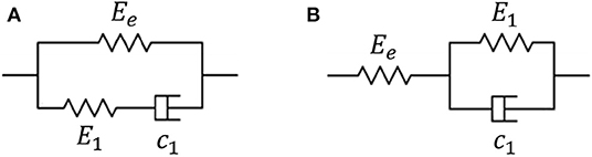
Figure 1. The standard linear solid model has two forms: Maxwell form (A) and Kelvin form (B). In this paper, the Maxwell form is used, and the term “standard linear solid model” means the Maxwell form of the standard linear solid model.

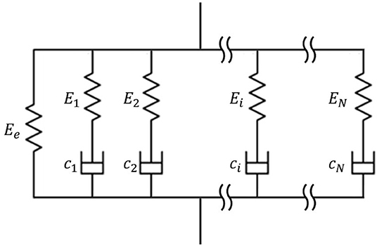
Figure 2. In the generalized Maxwell model, a spring and an arbitrary number of Maxwell bodies are connected in parallel. The standard linear solid model is a special case of the generalized Maxwell model with N = 1.

Although the standard linear solid model is a useful and easy-to-interpret model for analyzing viscoelastic behaviors, the analysis results (i.e., the obtained values of the three model parameters by curve fitting) cannot be directly compared to the parameters commonly adopted for defining the mechanical properties of viscoelastic solids. For example, in several finite element simulation packages, the modulus of elasticity as well as the parameters in the dimensionless form of the relaxation modulus, are used to define the mechanical properties of a linear viscoelastic solid. It introduces a problem that the parameters set in the finite element simulation package cannot be directly compared to those in the standard linear solid model, which is the model commonly used to curve fit the experimentally measured stress relaxation and creep curves. Since the parameters set in the finite element simulation package are often served as the standard for defining the mechanical properties of a linear viscoelastic solid, it is important to evaluate these parameters based on the experimental analysis results. In some applications, it is also important to compare the experimental and simulation results for the purpose of validation, as will be discussed in the Discussion section.

The main purpose of this paper is to introduce an alternative form of the standard linear solid model in terms of the modulus of elasticity and the parameters in the dimensionless form of the relaxation modulus for characterizing stress relaxation and creep of viscoelastic solids. By using the alternative form to analyze data, the experimental results can be directly compared to the theoretical parameters set in the finite element simulation. In this paper, the proposed model is validated by finite element simulation. It is also applied to analyze the experimental data of real materials. The physical meanings of the parameters in the dimensionless form of the relaxation modulus are investigated. It will be shown that the physical meaning of a parameter in the dimensionless form of the relaxation modulus, g is associated with the ratio of viscous fluids to solids of a viscoelastic solid. The theoretical background of the generalized Maxwell model, the standard linear solid model and its solutions for stress relaxation and creep are reviewed in the Appendix.

Materials and Methods

Derivation of the Alternative Form of the Standard Linear Solid Model for Characterizing Stress Relaxation and Creep

Please firstly note that the standard linear solid model has two forms, Maxwell form and Kelvin form (Figure 1). In the following derivation, the Maxwell form is used.

The stress as a function of time during the stress relaxation test using a unit step strain function described by the standard linear solid model:

where τ₁ = c₁/E₁ is the relaxation time constant, and ϵ₀ is the constant strain during the stress relaxation test.

The strain as a function of time during the creep test using a unit step stress function described by the standard linear solid model:

where τ₂ = c₁(E₁ + E_e)/E₁E_e is the creep time constant (or called retardation time constant), and σ₀ is the constant stress during the creep test.

Please refer to the Appendix for the derivation and relevant concepts of Equations (1) and (2).

Dividing Equation (1) by ϵ₀, the relaxation modulus is defined as:

Equation (3) can be written as:

where E₀ is equal to E₁ + E_e. It is the relaxation modulus at the beginning of stress relaxation, and is the stiffness of the material.

E_e is the constant relaxation modulus after the material is totally relaxed as t → ∞, and is the modulus of elasticity of the material.

E₁ =_{E0 − Ee} can be interpreted as how much the relaxation modulus drops from the beginning of the stress relaxation to the steady state as t → ∞.

Figure 3 illustrates the physical interpretations of E₀, E_e, and E₁.

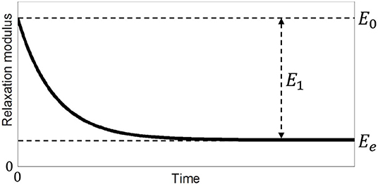
Figure 3. Illustration of E₀, E_e and E₁. E₀ is the relaxation modulus at the beginning of stress relaxation. E_e is the constant relaxation modulus as t → ∞, and is the modulus of elasticity of the material. E₁ can be interpreted as how much the relaxation modulus drops from the beginning of stress relaxation to the constant relaxation modulus as t → ∞.

Dividing Equation (4) by E₀, the dimensionless form of the relaxation modulus is:

where g = E₁/E₀ = E₁/(E_e + E₁), and g is a real number between 0 and 1. From this, the relationship between g (a parameter in the dimensionless form of the relaxation modulus), and E₁ and E_e (two parameters in the standard linear solid model) can be established.

In several finite element simulation packages, the modulus of elasticity E_e, and the two parameters g and τ₁ in the dimensionless form of the relaxation modulus, are used to define the mechanical properties of a linear viscoelastic solid.

Since g = E₁/(E_e + E₁), E₁ can be expressed as the function of g and E_e:

Substituting Equation (6) into Equation (1) yields:

It is the alternative form for describing the stress as a function of time during the stress relaxation test using a unit step strain function described by the standard linear solid model, in terms of g, E_e and τ₁.

Substituting Equation (6) into Equation (2) yields:

It is the alternative form for describing the strain as a function of time during the creep test using a unit step stress function described by the standard linear solid model, in terms of g, E_e and τ₂.

In practice, conventionally, we use the governing equation for the stress relaxation, i.e., Equation (1), or the governing equation for the creep, i.e., Equation (2), to curve fit the experimental stress relaxation or creep data for obtaining the three parameters in the standard linear solid model, E_e, E₁, and c₁. Next, we use the equation g = E₁/(E_e + E₁) to obtain the corresponding g, and use the definitions of the relaxation and creep time constants to obtain the two time constants. Now, we can directly use Equations (7) or (8) to curve fit the experimental stress relaxation or creep data to obtain the corresponding E_e, g and relaxation or creep time constants. By using this technique, we will be able to compare the experimental results (E_e, g, and τ₁ obtained from the experiment) to the theoretical parameters (E_e, g, and τ₁ set in the finite element simulation package). In this paper, finite element simulation is used to validate this proposed technique, as described in the next section.

Before closing this section, there are two important points to be addressed:

First, let's discuss the associated physical meaning of g. The physical meaning of g can be understood by examining Equation (4). There are two cases: first, if g → 1 as E₁ → E₀, f(t) drops to zero as t → ∞, and it means that the material contains more viscous fluids and less solids and behaves like a viscoelastic fluid; second, if g → 0 as E₁ → 0, f(t) remains a constant as t → ∞, and it means that the material behaves more like an elastic solid. Hence, g can be interpreted as a parameter governing the ratio of viscous fluids to solids of a viscoelastic solid. The more g closes to 1, the larger the ratio of viscous fluids to solids.

Second, let's discuss the relationship between the relaxation time constant τ₁ and creep time constant τ₂. From the definitions of τ₁ and τ₂, i.e., τ₁ = c₁/E₁, τ₂ = c₁(E₁ + E_e)/E₁E_e, and the equation g = E₁/(E_e + E₁), the relationship between τ₁, τ₂ and g can be obtained:

This equation demonstrates that the relaxation time constant is equal to 1−g times the creep time constant for the standard linear solid model. Since g is a real number between 0 and 1, Equation (9) implies that the creep time constant τ₂ is always larger than the relaxation time constant τ₁.

Finite Element Simulation

Finite element simulation was performed using ABAQUS/CAE 2019 (Dassault Systems Simulia Corp., Johnson, RI, USA) to validate the proposed alternative form of the standard linear solid model, i.e., Equations (7) and (8). The idea is to utilize the mechanical property parameters set in the computer simulation as the golden standard to validate the proposed Equations (7) and (8). More specifically, the simulation produces simulated stress relaxation and creep curves based on the set mechanical property parameters. Then, after using Equations (7) and (8) to curve fit the simulated stress relaxation and creep curves, respectively, the evaluated mechanical property parameters by curve fitting can be obtained. If the evaluated parameters are comparable to the parameters set in the computer simulation, the equations used for curve fitting can be validated to be effective. On the other hand, if the equations for curve fitting are not valid, the evaluated parameters by curve fitting will not be comparable to the parameters set in the computer simulation. Figure 4 illustrates the flowchart of this finite element simulation and numerical analysis.

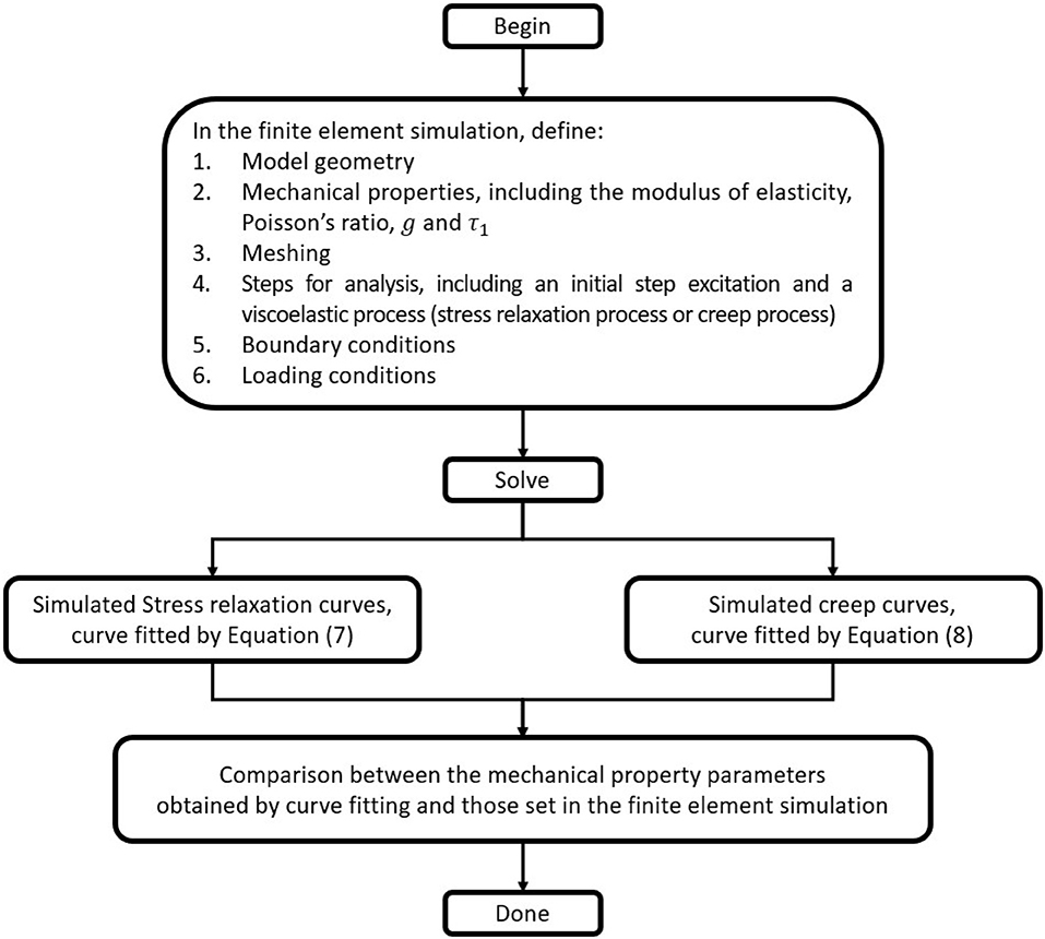
Figure 4. Flowchart of the finite element simulation and numerical analysis.

In the finite element simulation, an asymmetric homogeneous model was constructed for simulating the viscoelastic behaviors, including stress relaxation and creep, of a viscoelastic solid. The radius of the cross-sectional area and thickness of the model were 50 and 100 mm, respectively. The model was meshed by quadrilateral elements of dimensions 1.25 × 1.25 mm. The setting of the boundary conditions of the model was that the top and sides of the model were not fixed (i.e., displacements and rotations were allowed along all directions) while the bottom was fixed along the depth direction (i.e., displacements were not allowed along the depth direction, and rotations were not allowed along the lateral direction). The geometry and basic setting of the model are shown in Figure 5.

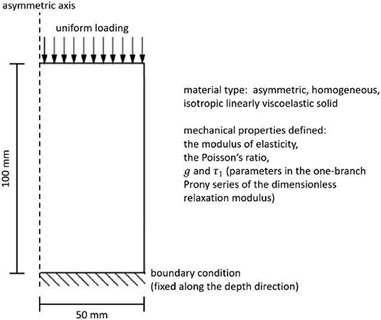
Figure 5. Geometry and basic setting of the model for the finite element simulation.

The model was constructed by an isotropic linearly viscoelastic solid. The mechanical properties of the material were defined by four parameters, including the modulus of elasticity (or called the Young's modulus), Poisson's ratio (set as 0.495 in this paper since the material was assumed to be incompressible), and the two parameters g and τ₁ in the one-branch Prony series of the dimensionless relaxation modulus in Equation (5).

In the stress relaxation simulation, the top edge of the model was uniformly applied by a deformation of the magnitude of 2.5 mm for a very short duration of 500 μs for simulating a step forcing function. The deformation was then kept constant at 2.5 mm until the stress response (i.e., the stress over time) of each element in the model reached the steady state. The stress and strain responses of all of the elements in the model were taken for analysis. The stress and strain responses along the depth direction of each element were collected, and then imported into MATLAB (R2019a; Mathworks, Natick MA) for analysis. Equation (7) was used to curve fit the stress response (i.e., stress relaxation curve) of each element for obtaining the corresponding E_e, g, and τ₁. During the curve fitting using Equation (8), ϵ₀ was taken as the strain value at the beginning of stress relaxation. The average value obtained from all of the elements for each parameter (E_e, g and τ₁) was used to compared to the theoretical value, i.e., the one set in ABAQUS during the simulation.

In the creep simulation, a uniform pressure was applied on the top edge of the model for a very short duration of 500 μs for simulating a step forcing function. The magnitude of pressure was such that the strain in the steady state was 5%. The pressure was then kept constant until the strain response (i.e., the strain over time) of each element in the model reached the steady state. Similar to the method used in the stress relaxation simulation, the stress and strain responses of each element were collected, and then imported into MATLAB for analysis. Equation (8) was used to curve fit the strain response (i.e., creep curve) of each element for obtaining the corresponding E_e, g and τ₂. During the curve fitting using Equation (8), σ₀ was taken as the stress value at the beginning of creep. Both g and τ₂ obtained by curve fitting and Equation (9) were used to obtain the corresponding τ₁. Similar to the method in the stress relaxation simulation, the average value for each parameter (E_e, g, and τ₁) was compared to the theoretical value set in ABAQUS during the simulation.

For each simulation scenario (stress relaxation or creep), three groups of materials were studied. In the first group, E_e = 1,000, 5,000, 10,000, 50,000, and 100,000 Pa while τ₁ = 5 s and g = 0.8. In the second group, τ₁ = 0.5, 1, 5, 10, and 20 s while E_e = 5,000 Pa and g = 0.8. Finally, in the third group, g = 0.01, 0.2, 0.4, 0.6, 0.8, 0.85, 0.9, 0.95, 0.99 while E_e = 5,000 Pa and τ₁ = 5 s. In each group, the value for each parameter obtained from the simulated curve by curve fitting was compared to the theoretical one set in ABAQUS.

Experimental Data Analysis

Equations (7) and (8) were used to curve fit the experimental data of stress relaxation and creep, respectively, for preliminarily investigating how the alternative form of the standard linear solid model works on the experimental data.

First, the stress relaxation behaviors of magnetorheological gels with different carbonyl iron particle concentrations (40, 50, 60, and 70 wt%) under shear loading (Figure 6A) were analyzed (curve fitted) by Equation (7). The data were reproduced from the paper by Xu et al. (2017). ϵ₀ in Equation (7) was set as 0.2% during the curve fitting (Xu et al., 2017). The three parameters, E_e, g, and τ₁, of each sample with a specific concentration obtained by curve fitting were descriptively reported.

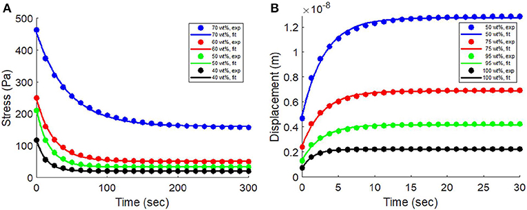
Figure 6. (A) The stress relaxation behaviors of magnetorheological gels with different carbonyl iron particle concentrations (40, 50, 60, and 70 wt%) were curve fitted by Equation (7). (B) The creep behaviors of nanocomposite thin films with different CdSe quantum dot concentrations (50, 75, 95, and 100 wt%) were curve fitted by Equation (8).

Second, the creep behaviors of nanocomposite thin films with different CdSe quantum dot concentrations (50, 75, 95, and 100 wt%) under nanoindentation (Figure 6B) were analyzed (curve fitted) by Equation (8). The data were reproduced from the paper by McCumiskey et al. (2010). σ₀ in Equation (8) was set as 24.3 μN during the curve fitting (McCumiskey et al., 2010). The three parameters, E_e, g, and τ₁, of each sample with a specific concentration obtained by curve fitting were descriptively reported.

Results

Results of the Finite Element Simulation

The finite element simulation results are shown in Table 1. The r² values for curve fitting of all of the cases were higher than 0.98. The results show that the values of E_e, g, and τ₁ obtained from the simulated curve by curve fitting were approximately equal to the theoretical ones (i.e., those set in ABAQUS) both for stress relaxation and creep. However, in the group 3, it can be observed that the error of τ₁ increased nonlinearly with increasing g (Figure 7). The error of τ₁ became significant when g approached 0.95 (error = 6.3 and 7.0% for stress relaxation and creep, respectively, when g = 0.95), and was unacceptable when g was larger than 0.95 (error = 33.0 and 41.6% for stress relaxation and creep, respectively, when g = 0.99). The results suggest that the alternative form of the standard linear solid model for characterizing stress relaxation and creep of viscoelastic solids, i.e., Equations (7) and (8), can accurately evaluate the corresponding E_e, g. and τ₁, except for a material with a value of g approximately larger than 0.95.

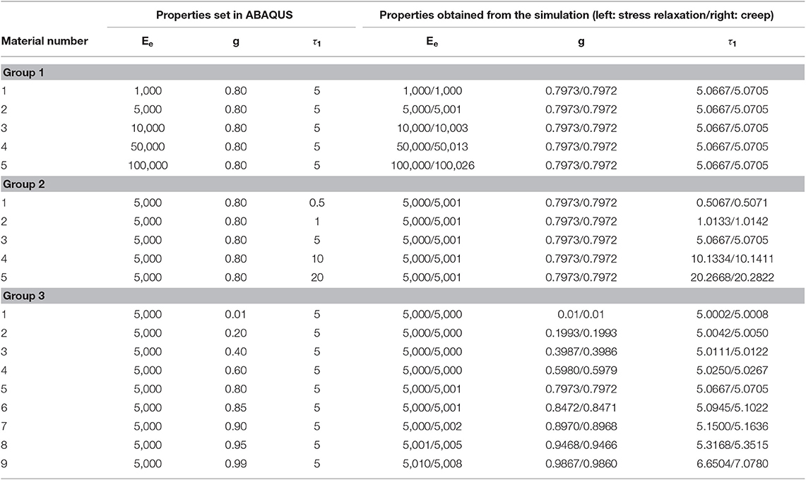
Table 1. Comparison between the values of properties set in ABAQUS and the ones obtained from the simulation.

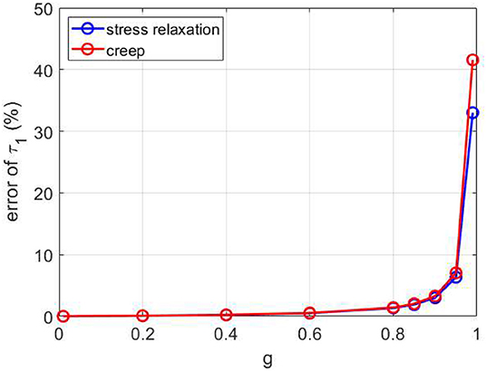
Figure 7. The error of τ₁ increased nonlinearly with increasing g.

Figure 8A shows several stress and strain responses over time of different materials in the group 3 during the stress relaxation test. Figure 8B shows the corresponding relaxation moduli. It should be reminded that the values of E_e and τ₁ were the same (E_e = 5,000 Pa and τ₁ = 5 s) while the g values were different for different materials in the group 3. It can be observed that the stress and relaxation modulus values at the beginning of stress relaxation were larger for larger g. The stress and relaxation modulus values after the material was totally relaxed were the same for different g. The strain responses were the same for different g. Figure 8C shows the corresponding dimensionless form of the relaxation moduli. It can be observed that the dimensionless relaxation modulus dropped more as t → ∞ for larger g, and dropped less for small g. For g = 0.01, the dimensionless relaxation modulus dropped just a little bit.

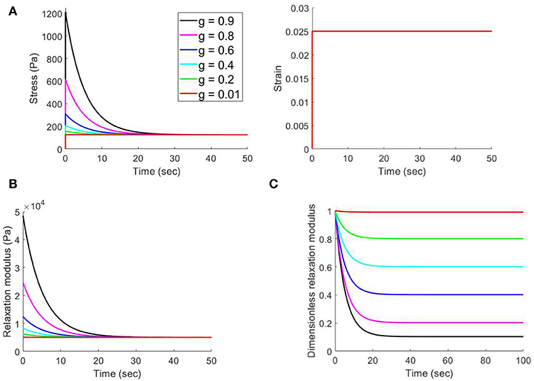
Figure 8. (A) Stress and strain responses over time of different materials in the group 3 during the stress relaxation test. (B) Corresponding relaxation moduli. (C) Corresponding dimensionless form of the relaxation moduli.

Figure 9A shows several stress and strain responses over time of different materials in the group 3 during the creep test. Figure 9B shows the corresponding creep compliance. It can be observed that the strain and creep compliance values at the beginning of creep were smaller for larger g. The strain and creep compliance values after the material was totally creeped were the same for different g. The stress responses were the same for different g.

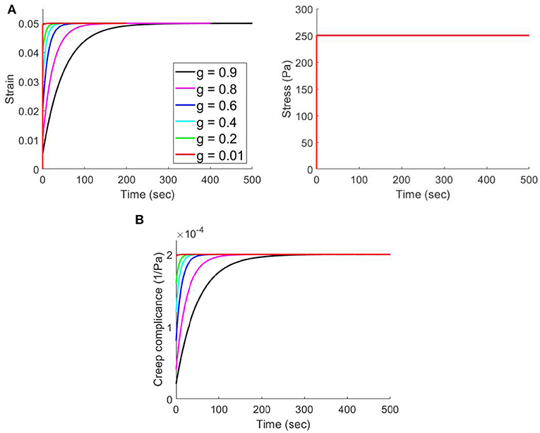
Figure 9. (A) Strain and stress responses over time of different materials in the group 3 during the creep test. (B) Corresponding creep compliance.

Results of the Experimental Data Analysis

Figure 6A shows that Equation (7) fitted the stress relaxation behaviors of magnetorheological gels quite well (the r² values for curve fitting of all of the cases were higher than 0.98). The values of E_e were 9.82, 16.7, 25.4, and 80.0 kPa, the values of g were 0.85, 0.84, 0.79 and 0.65, the values of τ₁ were 13.99, 18.15, 24.39 and 44.68 s, for carbonyl iron particle concentrations of 40, 50, 60, and 70 wt%, respectively. It means that the gel's modulus of elasticity increases, and ratio of viscous fluids to solids decreases with increasing particle concentrations.

Figure 6B shows that Equation (8) provided a very good fit to the creep behaviors of nanocomposite thin films (the r² values for curve fitting of all of the cases were higher than 0.98). The values of E_e were 1.91, 3.53, 5.80, and 11.0 kPa, the values of g were 0.61, 0.63, 0.66, and 0.67, the values of τ₁ were 3.11, 2.90, 2.78, and 1.54 s, for CdSe quantum dot concentrations of 50, 75, 95 and 100 wt%, respectively. It means that the film's modulus of elasticity increases, and ratio of viscous fluids to solids increases with increasing quantum dot concentrations.

Discussion

There are two main and important findings in the present study, as summarized and discussed in the next four paragraphs.

First, the alternative form of standard linear solid model introduced in the present study provides a link between the parameters in the traditional linear viscoelastic models (experimental results obtained by curve fitting the experimental data) and those in the dimensionless form of the relaxation modulus (theoretical parameters set in the finite element simulation package), so that they can be compared to each other. In some applications, it is very important to compare the parameters set in the finite element simulation package to those in the traditional standard linear solid model. For example, a technology for noninvasive measurement of the viscoelastic properties of materials is going to be developed. Before constructing the real system, it would be better to use finite element computer simulation to implement the theories and mechanisms of the technology to simulate the performance of the technology for understanding if it can accurately measure the viscoelastic properties of materials or not, according to the logic described below. First, the simulated data of viscoelastic behaviors (stress relaxation and creep curves) can be obtained from the computer simulation. Second, a viscoelastic model is used to curve fit the simulated viscoelastic behavior to obtain the corresponding viscoelastic properties. Third, if the evaluated viscoelastic properties obtained by curve fitting are similar to the ones set in the finite element simulation package during the computer simulation, it can be claimed that the design of the technology is proper; on the other hand, if the theories and mechanisms of the technology are not proper, the evaluated viscoelastic properties obtained by curve fitting will not be similar to the ones set in the finite element simulation package during the computer simulation. The problem is, the standard linear solid model frequently used to curve fit the data of viscoelastic behaviors is not the same as the model used to define the viscoelastic properties in the finite element simulation package (the dimensionless form of the relaxation modulus) such as ABAQUS, ANSYS and COMSOL and FEBio. Hence, the viscoelastic properties obtained by curve fitting cannot be compared directly to those set in the finite element simulation package. Since the alternative form is formulated in terms of the parameters used to define the mechanical properties in the finite element simulation package, the parameters obtained by curve fitting can be directly compared to those set in the finite element simulation package.

It should be emphasized again that the important role of the traditional standard linear solid model cannot be replaced. The purpose of using the alternative form is not to replace the traditional form. The main purpose of using the alternative form to curve fit the data is that, the parameters obtained by curve fitting can be compared directly to the parameters used to define the mechanical property parameters in the finite element simulation package. It is because the alternative form is formulated in terms of the parameters used to define the mechanical properties in the finite element simulation package. Or, researchers can also use the traditional standard linear solid model to curve fit the data, and then construct the parameters used to define the mechanical properties in the finite element simulation package by using the parameters in the traditional standard linear solid model (E_e E₁, and c₁), based on the equations g = E₁/(E_e + E₁) and τ₁ = c₁/E₁.

The other main finding is the introduction of the physical meaning of g. How g affects the behaviors of stress relaxation and creep curves was also studied. To the best knowledge, it could be the first time that the associated physical meaning of g is proposed. g is a parameter in the dimensionless form of the relaxation modulus used to define the linear viscoelastic properties in the simulation finite element simulation package. In the past, the physical meaning of g is unclear, therefore there would be a problem of setting the numerical value of this parameter during the simulation. In the present study, it was found that g is associated with the ratio of viscous fluids to solids of a viscoelastic solid; the more g closes to 1, the larger the ratio of viscous fluids to solids. This parameter can be applied to quantify the ratio of viscous fluids to solids of a viscoelastic solid, and could lead to many interesting and important applications. For example, this parameter can be used to determine the characteristics of biomaterials, since biomaterials with different characteristics may have different ratios of fluids to solids. This parameter can also be used to evaluate the degree of injury of a tissue, since tissues with different degrees of injuries may have different ratios of fluids to solids. Researchers can use the alternative form of the standard linear solid model introduced in the present study to calculate g. Or, researchers can measure E_e and E₁ of the traditional standard linear solid model firstly and then calculate g, since g = E₁/(E_e + E₁) as demonstrated in the present study.

The parameters in the traditional standard linear solid model are still important since they have clear physical meanings and are strictly related with the elastic and viscous properties (Shahidi et al., 2014, 2015a,b, 2016). Introducing the role of g is not for replacing the parameters in the traditional standard linear solid model, but is for providing another parameter having physical meaning that may have interesting and important application value.

The physical meaning of g_i in the generalized Maxwell model can be explained in a similar manner. Let's consider Equation (A.16) (Please see the Appendix), the dimensionless form of the relaxation modulus in the generalized Maxwell model:

Each $g_i\left(1-e^{-t/{\tau }_i}\right)$ in the equation can be interpreted as a viscoelastic component, corresponding to a local region of the material. Generally, the relaxation modulus of a viscoelastic solid can be described by Equation (A.16), consisting of many viscoelastic components. The more complicated the internal structure of a viscoelastic solid, the more non-linear the viscoelastic behavior and the more viscoelastic components the equation should have for describing the material behavior well. In each viscoelastic component $g_i\left(1-e^{-t/{\tau }_i}\right)$, g_i is the ratio of viscous fluids to solids in this component.

The relationship between the relaxation and creep time constants and g was also demonstrated, i.e., Equation (9). Since g is between 0 and 1, this equation shows that the creep time constant must be always larger than the relaxation time constant. It is an important fact, especially for an accurate parameter setting during numerical simulation. In some numerical simulation scenarios like dynamic viscoelasticity test, the properties that we intend to investigate are functions of the creep and relaxation time constants, such as the amplitude of the complex modulus and phase shift (Fung, 1993; Banks et al., 2011). Hence, we have to set the proper numerical values for the creep and relaxation time constants during simulation. Based on the finding, we must comprehend that the numerical value of the creep time constant must be larger than that of the relaxation time constant during the parameter setting of the simulation, or the simulation will produce an unreasonable result.

There are some interesting findings in Figure 8: (1) the stress and relaxation modulus values at the beginning of stress relaxation were larger for larger g, suggesting that the stiffness of the material is larger for larger g. This observation could be explained as follows. Both elastic property and fluid property can affect the stiffness of a material. The larger the modulus of elasticity and the larger amount of viscous fluid of a material, the larger the stiffness. Since g could be a parameter associated with the ratio of viscous fluids to solids of a viscoelastic solid, a viscoelastic solid with larger g means that this material contains a larger amount of viscous fluid that can increase the stiffness of this material when subjected to an external load. In other words, the increased stiffness with larger g is contributed by the larger viscous fluid effect, while the elastic property stays the same; (2) the stress and relaxation modulus values after the material was totally relaxed were the same for different g. It is because this long-term relaxation modulus is just the modulus of elasticity of the material. Since the modulus of elasticity was set as constant for each material during this simulation, the long-term relaxation modulus must be the same for each material; (3) the dimensionless relaxation modulus dropped more as t → ∞ for larger g, and dropped less for small g. This simulation results justifies our inference that g could be a parameter associated with the ratio of viscous fluids to solids of a viscoelastic solid. The more g closes to 1, the larger the ratio of viscous fluids to solids. On the other hand, the material behaves more like an elastic solid when g approaches zero. Similar explanations in (1) and (2) above can be used to explain the findings in Figure 9 for the creep test.

The use of the alternative form of the standard linear solid model for analyzing the experimental data shows interesting findings. For the stress relaxation behaviors of magnetorheological gels with different carbonyl iron particle concentrations, it was reasonable to find that the gel became stiffer and more like a solid when the particle concentration was higher. For the creep behaviors of nanocomposite thin films with different CdSe quantum dot concentrations, it was interesting to find that the film behaved more like a viscous fluidic material when the quantum dot concentration was higher, although the modulus of elasticity of the film increased with increasing quantum dot concentration as expected. In the future, the alternative form can be applied to analyze the viscoelastic behaviors of various biomaterials for better understanding their physical properties and the effects of mixtures.

There are some limitations in the present study. The first limitation is that, the physical meanings of the parameters in the alternative form of the standard linear solid model are demonstrated based on theories and derivations, combined with the known phenomena of behaviors of viscoelastic solids. In the future, rigorous experiments must be conducted to verify the physical meanings of the parameters. The second limitation is that, the relationship between g and the two elastic parameters in the standard linear solid model was derived in the present study, but not for the more general generalized Maxwell model. It is necessary to derive a similar relationship for the generalized Maxwell model for providing a more general model that can be applied to a wider variety of applications. The third limitation is that, the constitutive equations derived in this paper can only be applied when the input approaches a unit step function. It is necessary to derive a more general set of constitutive equations that can be applied when another type of input like a ramp input is used. The final limitation is that, linear viscoelastic models are not the most general models for describing the viscoelastic behaviors of materials. They can only be applied to analyze some specific types of materials. Quasi-linear and non-linear viscoelastic models, internal variable and finite differential models, are more general for describing viscoelastic behaviors of most materials (Wineman, 2009; Chatelin et al., 2010; Rashid et al., 2014). Despite the limited application of linear viscoelastic models, they are still useful from two different points of view. First, they are still useful and widely applied to describe the viscoelastic behaviors of a variety of materials like biomaterials, polymers and biological tissues having simpler structures, especially in applications where the material strain is tiny such as that induced by ultrasound (Deng et al., 2016; Hong et al., 2016, 2018) and photoacoustic imaging (Ishihara et al., 2003). Second, since the mathematics for understanding linear viscoelastic theory is much simpler, it is a nice first step for newcomers to learn viscoelastic theory and apply to describe viscoelastic behaviors of materials.

Conclusions

In conclusion, the alternative form is formulated in terms of the parameters used to define the mechanical properties in the finite element simulation package, so that the parameters obtained by curve fitting can be directly compared to those set in the finite element simulation package. It was also found that, the physical meaning of g, a parameter in the dimensionless form of the relaxation modulus, is associated with the ratio of viscous fluids to solids of a viscoelastic solid. Quantifying the ratio of viscous fluids to solids of a viscoelastic solid could lead to many interesting and important applications. In the future, a rigorous experiment will be conducted to verify the physical meanings of the parameters in the alternative form. It is planned to make several gel phantoms having different fluid contents and viscoelastic properties. The modulus of elasticity, stress relaxation and creep curves of each phantom will be measured by a material testing machine, and the fluid content will be measured by a moisture analyzer. The parameters in the alternative form of each phantom can be obtained after using the alternative form to curve fit the stress relaxation and creep curves. The physical meaning of each parameter can be verified by investigating the correlation between the values of parameter obtained by curve fitting and associated physical quantity measured by the associated instrument.

Data Availability Statement

The datasets generated for this study are available on request to the corresponding author.

Author Contributions

C-YL was responsible for conceptualization, design, theory, investigation, and writing.

Funding

The research was financially supported by the Ministry of Science and Technology of Taiwan (grant number: MOST 108-2218-E-002-046-MY3).

Conflict of Interest

The author declares that the research was conducted in the absence of any commercial or financial relationships that could be construed as a potential conflict of interest.

Supplementary Material

The Supplementary Material for this article can be found online at: https://www.frontiersin.org/articles/10.3389/fmats.2020.00011/full#supplementary-material

References

Agarwal, R., and García, A. J. (2015). Biomaterial strategies for engineering implants for enhanced osseointegration and bone repair. Adv. Drug Deliver. Rev. 94, 53–62. doi: 10.1016/j.addr.2015.03.013
Banks, H. T., Hu, S., and Kenz, Z. R. (2011). A brief review of elasticity and viscoelasticity for solids. Adv. Appl. Math. Mech. 3, 1–51. doi: 10.4208/aamm.10-m1030
Braunsmann, C., Proksch, R., Revenko, I., and Schäffer, T. E. (2014). Creep compliance mapping by atomic force microscopy. Polymer 55, 219–225. doi: 10.1016/j.polymer.2013.11.029
Cacopardo, L., Guazzelli, N., Nossa, R., Mattei, G., and Ahluwalia, A. (2019). Engineering hydrogel viscoelasticity. J. Mech. Behav. Biomed. 89, 162–167. doi: 10.1016/j.jmbbm.2018.09.031
Chatelin, S., Constantinesco, A., and Willinger, R. (2010). Fifty years of brain tissue mechanical testing: from in vitro to in vivo investigations. Biorheology 47, 255–276. doi: 10.3233/BIR-2010-0576
Chester, S. A. (2012). A constitutive model for coupled fluid permeation and large viscoelastic deformation in polymeric gels. Soft Matter 8, 8223–8233. doi: 10.1039/c2sm25372k
Deng, C. X., Hong, X., and Stegemann, J. P. (2016). Ultrasound imaging techniques for spatiotemporal characterization of composition, microstructure, and mechanical properties in tissue engineering. Tissue Eng. Part B Rev. 22, 311–321. doi: 10.1089/ten.TEB.2015.0453
Diego, R. B., Estellés, J. M., Sanz, J. A., García-Aznar, J. M., and Sánchez, M. S. (2007). Polymer scaffolds with interconnected spherical pores and controlled architecture for tissue engineering: fabrication, mechanical properties, and finite element modeling. J. Biomed. Mater. Res. B Appl. Biomater. 81, 448–455. doi: 10.1002/jbm.b.30683
Feng, Z., Seya, D., Kitajima, T., Kosawada, T., Nakamura, T., and Umezu, M. (2010). Viscoelastic characteristics of contracted collagen gels populated with rat fibroblasts or cardiomyocytes. J. Artif. Organs 13, 139–144. doi: 10.1007/s10047-010-0508-x
Fung, Y. C. (1993). Biomechanics: Mechanical Properties of Living Tissues. New York, NY: Springer Science & Business Media.
Hong, X., Annamalai, R. T., Kemerer, T. S., Deng, C. X., and Stegemann, J. P. (2018). Multimode ultrasound viscoelastography for three-dimensional interrogation of microscale mechanical properties in heterogeneous biomaterials. Biomaterials 178, 11–22. doi: 10.1016/j.biomaterials.2018.05.057
Hong, X., Stegemann, J. P., and Deng, C. X. (2016). Microscale characterization of the viscoelastic properties of hydrogel biomaterials using dual-mode ultrasound elastography. Biomaterials 88, 12–24. doi: 10.1016/j.biomaterials.2016.02.019
Ishihara, M., Sato, M., Sato, S., Kikuchi, T., Fujikawa, K., and Kikuchi, M. (2003). Viscoelastic characterization of biological tissue by photoacoustic measurement. Jpn. J. Appl. Phys. 42:L556. doi: 10.1143/JJAP.42.L556
McCumiskey, E. J., Chandrasekhar, N., and Taylor, C. R. (2010). Nanomechanics of CdSe quantum dot–polymer nanocomposite films. Nanotechnology 21:225703. doi: 10.1088/0957-4484/21/22/225703
O'Brien, F. J. (2011). Biomaterials & scaffolds for tissue engineering. Mate. Today 14, 88–95. doi: 10.1016/S1369-7021(11)70058-X
Plaseied, A., and Fatemi, A. (2008). Deformation response and constitutive modeling of vinyl ester polymer including strain rate and temperature effects. J. Mater. Sci. 43, 1191–1199. doi: 10.1007/s10853-007-2297-z
Rashid, B., Destrade, M., and Gilchrist, M. D. (2014). Mechanical characterization of brain tissue in tension at dynamic strain rates. J. Mech. Behav. Biomed. Mater. 33, 43–54. doi: 10.1016/j.jmbbm.2012.07.015
Sethuraman, V., Makornkaewkeyoon, K., Khalf, A., and Madihally, S. V. (2013). Influence of scaffold forming techniques on stress relaxation behavior of polycaprolactone scaffolds. J. Appl. Polymer Sci. 130, 4237–4244. doi: 10.1002/app.39599
Shahidi, M., Pichler, B., and Hellmich, C. (2014). Viscous interfaces as source for material creep: a continuum micromechanics approach. Eur. J. Mech. A. Solids 45, 41–58. doi: 10.1016/j.euromechsol.2013.11.001
Shahidi, M., Pichler, B., and Hellmich, C. (2015a). Interfacial micromechanics assessment of classical rheological models. I: single interface size and viscosity. J. Eng. Mech. 142:04015092. doi: 10.1061/(ASCE)EM.1943-7889.0001012
Shahidi, M., Pichler, B., and Hellmich, C. (2015b). Interfacial micromechanics assessment of classical rheological models. II: multiple interface sizes and viscosities. J. Eng. Mech. 142:04015093. doi: 10.1061/(ASCE)EM.1943-7889.0001013
Shahidi, M., Pichler, B., and Hellmich, C. (2016). How interface size, density, and viscosity affect creep and relaxation functions of matrix-interface composites: a micromechanical study. Acta Mech. 227, 229–252. doi: 10.1007/s00707-015-1429-9
Shazly, T. M., Artzi, N., Boehning, F., and Edelman, E. R. (2008). Viscoelastic adhesive mechanics of aldehyde-mediated soft tissue sealants. Biomaterials 29, 4584–4591. doi: 10.1016/j.biomaterials.2008.08.032
Smith, B. D., and Grande, D. A. (2015). The current state of scaffolds for musculoskeletal regenerative applications. Nat. Rev. Rheumatol. 11, 213–222. doi: 10.1038/nrrheum.2015.27
Stammen, J. A., Williams, S., Ku, D. N., and Guldberg, R. E. (2001). Mechanical properties of a novel PVA hydrogel in shear and unconfined compression. Biomaterials 22, 799–806. doi: 10.1016/s0142-9612(00)00242-8
Tirella, A., Mattei, G., and Ahluwalia, A. (2014). Strain rate viscoelastic analysis of soft and highly hydrated biomaterials. J. Biomed. Mater. Res. 102, 3352–3360. doi: 10.1002/jbm.a.34914
Vedadghavami, A., Minooei, F., Mohammadi, M. H., Khetani, S., Kolahchi, A. R., Mashayekhan, S., et al. (2017). Manufacturing of hydrogel biomaterials with controlled mechanical properties for tissue engineering applications. Acta Biomate. 62, 42–63. doi: 10.1016/j.actbio.2017.07.028
Wineman, A. (2009). Nonlinear viscoelastic solids—a review. Math. Mech. Solids 14, 300–366. doi: 10.1177/1081286509103660
Wright, L. D., Andric, T., and Freeman, J. W. (2011). Utilizing NaCl to increase the porosity of electrospun materials. Mat. Sci. Eng. C 31, 30–36. doi: 10.1016/j.msec.2010.02.001
Xiao, R., Sun, H., and Chen, W. (2016). An equivalence between generalized maxwell model and fractional zener model. Mech. Mater. 100, 148–153. doi: 10.1016/j.mechmat.2016.06.016
Keywords: viscoelasticity, mechanical properties, generalized Maxwell model, relaxation modulus, biomaterials, finite element simulation
Citation: Lin C-Y (2020) Alternative Form of Standard Linear Solid Model for Characterizing Stress Relaxation and Creep: Including a Novel Parameter for Quantifying the Ratio of Fluids to Solids of a Viscoelastic Solid. Front. Mater. 7:11. doi: 10.3389/fmats.2020.00011
Received: 04 September 2019; Accepted: 13 January 2020;
Published: 06 February 2020.
Edited by:
Federico Bosia, Politecnico di Torino, ItalyReviewed by:
Rostand Moutou Pitti, Université Clermont Auvergne, FranceMassimiliano Zingales, University of Palermo, Italy
Copyright © 2020 Lin. This is an open-access article distributed under the terms of the Creative Commons Attribution License (CC BY). The use, distribution or reproduction in other forums is permitted, provided the original author(s) and the copyright owner(s) are credited and that the original publication in this journal is cited, in accordance with accepted academic practice. No use, distribution or reproduction is permitted which does not comply with these terms.
*Correspondence: Che-Yu Lin, cheyu@ntu.edu.tw