Numerical Validation of Multiphysic Imperfect Interfaces Models
 Serge Dumont
 Michele Serpilli2
  Raffaella Rizzoni
 Frédéric C. Lebon
- 1IMAG CNRS UMR 5149, University of Nîmes, Nîmes, France
- 2Department of Civil and Building Engineering and Architecture, Università Politecnica delle Marche, Ancona, Italy
- 3Department of Engineering, University of Ferrara, Ferrara, Italy
- 4Aix-Marseille Univ, CNRS, Centrale Marseille, LMA, Marseille, France
We investigate some mathematical and numerical methods based on asymptotic expansions for the modeling of bonding interfaces in the presence of linear coupled multiphysic phenomena. After reviewing new recently proposed imperfect contact conditions (Serpilli et al., 2019), we present some numerical examples designed to show the efficiency of the proposed methodology. The examples are framed within two different multiphysic theories, piezoelectricity and thermo-mechanical coupling. The numerical investigations are based on a finite element approach generalizing to multiphysic problems the procedure developed in Dumont et al. (2018).
1. Introduction
The design of composite materials and structures is nowadays characterized by an increasing level of complexity regarding their heterogeneous morphology and constitution in order to attain more reliable and multi-functional performances in extreme environments. Even though advances have been made in the understanding of the mechanical behavior of composite materials, their synergistic response in a multi-physical environment is not yet fully understood. Composites as well as bonded structures are obtained by joining different parts with highly contrasted mechanical properties to compose a unique assembly. The bonded joint may generally be imperfect and discontinuities in the involved physical fields can arise, drastically changing the overall mechanical response (see, e.g., Gu and He, 2011; Gu et al., 2014; Javili et al., 2014). Therefore, a rigorous modeling of the imperfect bonding plays an important role in engineering design.
In the present paper, we analyze a particular composite constituted by a three bodies: namely, two adherents separated by a thin adhesive interphase. The composite assembly domain depends on a small parameter ε, corresponding to the constant thickness of the intermediate layer, called the adhesive. In order to take into account general multiphysic interactions among various physical behaviors, such as elasticity, magneto-electricity, thermal conduction, the constituents are made of general linear multiphysic materials.
Classically, the thin adhesive can be replaced by an interface law, as its thickness ε tends to zero. In the limit, the two adherents are joined by a limit surface, across which non-classical contact conditions are given to reproduce the behavior of the thin adhesive. Because the numerical treatment of a thin adhesive layers needs a very fine discretization, a 3D-2D model based on the introduction of the interface law is advantageous, requiring a much lower computation cost.
In the last years, various interface models have been proposed based on phenomenological or micromechanical approaches. On one hand, phenomenological models can be deduced directly from experiments. For example, effective non-linear interface phenomenological models have been proposed, among the others, in Fouchal et al. (2009), Lotfi and Shing (1994), and Lourenço and Rots (1997) for the analysis of masonry walls. On the other hand, interface models obtained through the asymptotic methods (see Ciarlet, 1997 for an extensive discussion) can be regarded as micromechanical models linking the interface response to the behavior of the material layer constituting the bonding, cf. Klarbring, 1991; Benveniste and Miloh, 2001; Hashin, 2002. The asymptotic analysis is a powerful mathematical technique, employed to justify classical thin structures and layered composites model (Ciarlet, 1997; Geymonat et al., 1999, 2014; Serpilli and Lenci, 2012, 2016; Serpilli, 2017). According to these techniques, the thickness of the glue is considered as a small parameter ε and, possibly, its stiffness depends on εp, where p is a critical exponent. Letting ε tend to zero, the adhesive layer geometrically vanishes, reducing itself to a 2D surface, but it is accounted for by a relation linking the jumps of the traction and the displacement vectors at the interface. Another benefit of a simplified 3D-2D model based on an interface law is the possibility of incorporating multiphysic materials behavior, spanning from uncoupled phenomena, such as thermal conduction and elasticity (Lebon and Rizzoni, 2010, 2011; Bessoud et al., 2011; Rizzoni et al., 2014; Raffa et al., 2018), to multifield and multiphysic theories, such as piezoelectricity and continua with microstructure, cf. Serpilli, 2015, 2017, 2018, 2019; Serpilli et al., 2019 and the references herein.
The aim of this paper is to numerically validate the general imperfect contact conditions derived in Serpilli et al. (2019), simulating the behavior of a thin interphase undergoing linear coupled multiphysic phenomena. As already stressed in Serpilli et al. (2019), the proposed multiphysic interface law, obtained through the asymptotic methods, provides a generalized transmission condition which contains in itself the soft (also called Kapitza's or lowly-conducting), hard (perfect), and rigid (Gurtin-Murdoch's or highly-conducting) interface models. Our analysis is limited to the case of linear elastic response of the adhesive and adherents and the modeling is framed in the contest of small strains and small displacements theory. Then, some examples are given in order to show the efficiency of the proposed methodology in the case of piezoelectric and thermo-mechanical couplings. The numerical investigations are performed in the framework of the finite element method, generalizing the approach developed in Dumont et al. (2018) to multiphysic problems. In particular, finite elements are introduced to solve the fully 3D initial problem, considering a three-phase composite, and the limit 3D-2D problem with two layers with imperfect interface transmission conditions.
Finally, the current model is limited to the case of a multiphysics linear elastic response of the adhesive and the adherents. However, using the techniques proposed in Bonetti et al. (2017), Raffa et al. (2018), and Rizzoni et al. (2017), it could be extended to more general frameworks, like the non-linear regime or damaging adhesives with behavior governed by the evolution of the crack length at the micro-scale. These extensions will be the topics of further study.
2. The General Theory
In this section, some results previously obtained are recalled. We consider the assembly constituted of two solids , called the adherents, bonded together by an intermediate thin layer of thickness ε, 0 < ε < 1, called the adhesive, with cross-section S ⊂ ℝ2. In the following Bε and S will be called interphase and interface, respectively. Let be the plane interfaces between the interphase and the adherents and let denote the composite system comprising the interphase and the adherents.
We suppose that the composite is constituted of a material which presents a linear coupled multiphysic behavior. The state at the equilibrium of the multiphysic material is characterized by a collection of order parameters, using the multifield theory jargon (see, e.g., Mariano, 2002): N vector state variables, namely , and M scalar state variables, namely . Let us collect all the unknowns into a generalized vector field , the so-called multiphysic state. With the multiphysic state sε, we associate its conjugated physical quantity tε = tε(∇εsε), depending on the gradient of sε, defined by . The vector field represents a generalized stress field.
We consider the following homogeneous and linear constitutive law:
where Kε is a generalized linear constitutive matrix, that we can write, component-wise,
with J, K = 1, …, N and I, L = 1, …, M and using Einstein's notations. The constitutive tensor Kε satisfies the classical symmetry and positivity properties.
A straight-forward example of such behavior is represented by piezoelectricity, in which an electric field is generated by a mechanical strain (direct effect) and, viceversa, a mechanical strain is produced as a result of an electric field (converse effect). The piezoeletric state consists of a pair s = (u, φ), namely the displacement field u = (ui) and the electric potential φ. The constitutive law takes the form takes the form:
where is the linearized strain tensor, D = (Di) represent the electric displacement field, E: = −∇φ represent the electric field, while C = (Cijkℓ), P = (Pijk) and H = (Hij) denote, respectively, the elasticity tensor, the piezoelectric coupling tensor and the dielectric tensor. In this case, tensor K reduces to
Any other multiphysic behavior can be generalized by adding other possible couplings within the constitutive law, coming from different physical interactions, as in magneto-electro-thermo-elastic materials (see, e.g., Serpilli, 2017, 2018).
It is assumed that the adherents are subject to a generalized system of body forces and surface forces , where . Body and surface forces are neglected in adhesive layer. On homogeneous boundary conditions are prescribed, so that sε = 0 on . We assume that everywhere, near the interphase boundary , homogeneous Neumann boundary conditions are applied. It is assumed that the adhesive and the adherents are perfectly bonded in order to ensure the continuity of the multiphysic state and generalized stress vector fields across . The differential (strong) formulation of the governing equations has the following structure:
where represents the generalized traction vector on the boundary and nε the outer normal unit vector to . We take V(Ωε) to denote the space of state variables admissible fields. The weak formulation of problem (2) defined on the variable domain Ωε is:
for all , where the bilinear forms , and Âε(·, ·) and the linear form Lε(·) are defined by
In the sequel, the following notations are used:
The asymptotic behavior of problem (3), i.e., when ε → 0 is studied. The first step of the approach given by Ciarlet (1997) is to introduce a rescaling given by
where, after the change of variables, the adherents occupy and the interphase . The sets denote the interfaces between B and Ω± and Ω = Ω+∪Ω−∪B is the rescaled configuration of the composite. Lastly, Γg and Γu indicate the images through πε of and . Consequently, and in Ω±, and and in B. It is assumed that the constitutive coefficients of are independent of ε, so that while the constitutive coefficients of Bε present the following dependences on ε, so that with p ∈ {−1, 0, 1}. Three different limit behaviors will be characterized according to the choice of the exponent p: in the case of p = −1, we derive a model for a rigid interface; when p = 0, we derive a model for a hard interface; by choosing p = 1, we deduce a model for a soft interface. By virtue of classical hypothesis, the rescaled problem can be written in the following form:
for all r ∈ V(Ω), the set of rescaled admissible fields, where the bilinear forms Ā±(·, ·), â(·, ·), and ĉ(·, ·) are defined by
and denote the sub-matrices of , defined by
At this level, one can perform an asymptotic analysis of the rescaled problem (4), introducing the asymptotic expansions of the solution as a series of powers of ε:
where and , by substituting (5) into the rescaled problem (4), and by identifying the terms with identical power of ε, we can recover the limit problems at order 0 and order 1. Finally, matching conditions are introduced based on the continuity of the generalized traction and multiphysic state sε at the interfaces in the initial configuration and on the continuity of the traction and state , , , at the interfaces S± in the rescaled configuration (see Rizzoni et al., 2014; Dumont et al., 2018).
2.1. The Soft Multiphysic Interface Model
In the limit case p = 1, the adhesive is weaker than the adherents and the transmission problems at order 0 and order 1 can be summarized as follows (Serpilli et al., 2019):
• Order 0
• Order 1
2.2. The Hard Multiphysic Interface Model
When p = 0, the limit model corresponds to a hard multiphysic interface,. The order 0 and order 1 interface transmission problems are presented in the sequel (Serpilli et al., 2019):
• Order 0
• Order 1
2.3. The Rigid Multiphysic Interface Model
A rigid multiphysic interface can be obtained for p = −1. The order 0 and order 1 limit interface models are the following ones (Serpilli et al., 2019):
• Order 0
• Order
Note that it is possible to obtain a condensed form of transmission conditions, summarizing both the orders 0 and 1 of the soft and hard cases in only one couple of equations, in terms of the jump of the displacement field and tractions at the interface (Rizzoni et al., 2014). To this end, we denote by and , two suitable approximations for and . The rigid multiphysic interface conditions are considered. Let in Bε, we can write and , as
An alternative expression of the above transmission conditions can be given in terms of and , which will be useful to write the variational formulation of the interface multiphysic problem:
The variational formulation of the general multiphysic interface problem is given by Serpilli et al. (2019):
for all , where is the set of admissible fields, with and
where denotes the load on the lateral boundary of the interface, which can be evaluated. By virtue of the Lax-Milgram lemma, we can infer that the interface variational problem (6) admits one and only one solution (see Serpilli et al., 2019, for more details).
3. Numerical Validation of the Generalized Interface Conditions
This Section is devoted to the numerical implementation of the generalized interface conditions, identified in Serpilli et al. (2019) and expressed by means of the transmission problem (6). The numerical simulations will help to prove the numerical performance of the proposed asymptotic approach. The above problem is numerically solved through the finite element method by considering a multiphysic composite constituted by two parallelepiped adherents separated by a thin adhesive, subject to general loading conditions. The analysis is carried out by choosing two particular multiphysic constitutive laws, corresponding to the case of piezoelectricity and thermo-elasticity. Finally, the numerical solution of the three-phase model (two adherents and adhesive) is compared with the numerical solution provided by the generalized interface problem (6), obtained by means of the asymptotic methods. These simple examples can be employed to model and understand the mechanical behavior of real laminated structures presenting multiphysic couplings such as piezoelectric stack actuators, piezo-patch sensor glued on a controlled substructure (see, for instance, Geis et al., 2004).
The numerical simulations hereinafter are performed using a finite element method to solve the weak problem (6). For that purpose, standard piecewise linear finite element are considered. As in the description of the interface model, the multiphysic variables are considered using a generalized variable s, leading to a fully coupled problem.
Finally, the problem is solved employing the software GetFem++ (see Renard and Pommier, 2002; Geuzaine and Remacle, 2009 for more details), with a standard linear solver (conjugate gradient).
3.1. The Piezoelectric Case
A piezoelectric material represents one of the most peculiar multiphysic material, combining the linear elastic behavior with the electric counterpart. As mentioned in section 2, the piezoeletric state reduces to a pair s = (u, φ), constituted by the displacement field u = (ui) and the electric potential φ. The constitutive law takes the form (1).
In what follows, we define the geometrical and physical settings of the numerical simulations. Let us consider a piezoelectric laminated plate occupying a 3D domain defined by Ω = [0, L1] × [0, L2] × [−h/2, h/2], with L1 = 10h and L2 = 5h (see Figure 1).
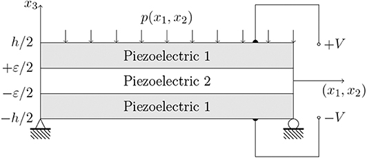
Figure 1. The 3D geometry of the piezoelectric laminated plate represented in the plane (x1, x3).
The adherents (Piezoelectric 1) are constituted by PVDF (Polyvinylidene fluoride), a monoclinic piezoelectric material with poling axis e3, while the adhesive (Piezoelectric 2) is made of PZT-4, a transversally isotropic piezoelectric material with poling axis e3, whose mechanical properties are shown in Table 1 (Fernades and Pouget, 2002). The constitutive sub-matrices (𝕂ij) are defined as follows:
For a transversally isotropic material with poling axis e3, one has c11 = c22, c13 = c23, c55 = c44, c66 = (c11 − c12)/2, e15 = e24, e31 = e32 and H11 = H22.
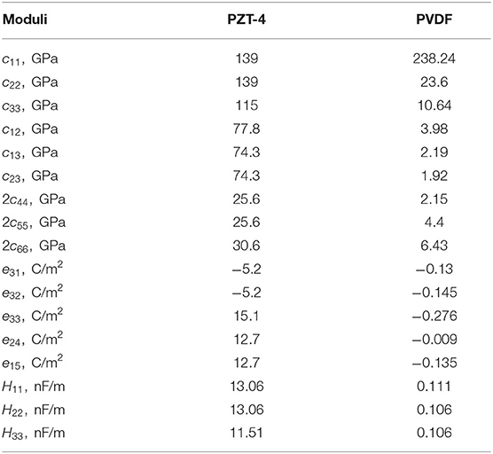
Table 1. Piezoelectric material properties for PZT-4 and PVDF, Fernades and Pouget (2002).
3.1.1. Numerical Results: The Applied Electric Potentials
The FEM discretization is carried out using P1 finite elements (linear on thetrahedrons), with 6552 nodes (27187 degrees of freedom) for the three-phases problem and 5824 nodes (24275 degrees of freedom) for the problem with the generalized interface law.
In this section, we study the case of two electric potentials V0 = ±25V, applied on both the upper and the lower faces of the composite plate (see Figure 1). No mechanical loading is considered in this example. The piezoelectric laminated plates behaves as a piezoelectric actuator.
Following the ideas proposed in Fernades and Pouget (2002), the numerical results for the variables are provided using the dimensionless units. For an applied electric potential V0, we set:
where, for numerical convenience, and C00 = 1GPa.
First, the influence of the relative thickness of the interphase is investigated in order to evaluate the accuracy of the asymptotic modeling. In particular, the quality of the solutions is evaluated considering the L2-relative error , where sε denotes the reference solution computed using the three-phases problem with a sufficiently fine finite element mesh to ensure a good approximation of the solution, while smodel indicates the solution of the interface model (6). Let us notice that the mesh does not depend on the thickness ε for the interface model, on the contrary of the computation of the reference solution, where the meshing of the interphase is necessary. The convergence of the general interface model toward the three-phases one with respect to the thickness ratio is presented in Figure 2.
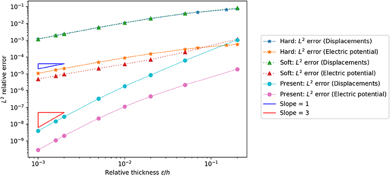
Figure 2. Convergence results with respect to the relative thickness ε/h.
From the plot, it can be observed that, by reducing the thickness of the adhesive, the relative error has a drastic reduction and so, the proposed general interface model provides an acceptable solution and it is able to correctly approximate the solution sε (see Bonnet et al., 2016). The convergence rate is (ε/h)3 and is consistent with expectancy. Besides, even if the relative thickness is of 1%, the relative error is close to 7.05 · 10−4 for the displacement field and close to 2.42 · 10−5 for the electric potential, meaning that the general interface model can also be used for moderately thick adhesive layers.
In Figure 2, we also compared the solutions of the generalized interface conditions with some other classical interface models, namely, the hard and soft interfaces. Firstly, we consider the model, referenced as hard model, where the displacements and the electrical potential fields, and the traction vector and normal electric displacement at the interface are considered as continuous. Hence, the hard interface can be considered perfect. This case is obtained with asymptotic expansions method at order 0, when the materials properties in the interphase are independent of the parameter ε, and thus they have similar rigidities with respect to the adherents (see the equations at order 0 in section 2.2). In addition, we present the results obtained by the so-called soft model, obtained with asymptotic expansions at order 0 when the interphase material properties depend linearly on the parameter ε. In the soft case, it can be shown that the interface behaves as a linear multiphysic spring, where only the first term of the bilinear form is considered in the interface model (6) (see, also, equations at order 0 in section 2.1). Figure 2 shows that the present modeling significantly improve the quality of the approximation, even for large ε: the trend of the L2-relative error convergence rate, both for the displacements and the electric potential field, is passing from ε/h to (ε/h)3. This means that the solution of the three-phases model converges more quickly toward the solution of the present reduced model, as ε tends to zero, then the solution of the classical hard or soft interface models. Moreover, it is important to stress that the current generalized multiphysic interface model has been built in order to adapt itself to the any kind of adhesive, since it comprises and also improve both the hard and soft cases, taking into account higher order terms, see Serpilli et al., 2019 for a detailed discussion.
We now present a comparison between the solutions obtained on the three-phases problem and on the asymptotic approximations. In this case, the relative thickness of the interface is equal to 0.1, and the relative error is equal to 0.04% in terms of displacements and is equal to 10−3% in terms of electric potential. In the sequel, the plots of the solutions (Ui, Φi) are represented on the orthogonal line to the interface mid-plane defined by (x1 = L1/2, x2 = L2/2, x3/h ∈ [−0.5, 0.5]), while the jumps of the various physical quantities are plotted on the lines parallel to the interface mid-plane, namely (x1 ∈ [0, L1], x2 = L2/2, x3 = 0) and (x1 = L1/2, x2 ∈ [0, L2], x3 = 0).
Figure 3 represents the trend of the displacement field and electric potential, evaluated on the central orthogonal fiber to the mid-plane of the interface. The plot shows a very good agreement between the solution of the general interface problem (dotted line) and the solution of the three-phases problem (solid line). The composite plate behaves mostly as a Kirchhoff–Love single-layer plate, taking also into account the transversal deformation of the adhesive. From the electric point of view, the electric potential is linear through the adherents and constant through the adhesive: this is due to the fact that the intermediate layer (PZT-4) has a higher electrical conductivity with respect to upper and lower bodies (PVDF), see Table 1, and, hence, it behaves as a highly conducting interface.
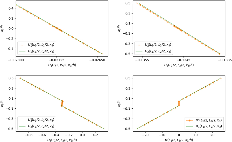
Figure 3. Displacement field and electric potential on a section along the x3 axis, with ε/h = 0.1.
Figures 4, 6 represent the trend of the jumps of the displacement and electric potential and the jumps of the traction vector and normal electric displacement along the x1-axis, namely (x1 ∈ [0, L1], x2 = L2/2, x3 = 0), and Figures 5, 7 along the x2-axis, namely (x1 = L1/2, x2 =∈ [0, L2], x3 = 0). The numerical simulations highlight that the proposed model is able to describe the mechanical behavior of the composite. Few solution oscillations can be found close to the lateral boundaries, due to the presence of edges, which produce expected stress concentrations and singularities.
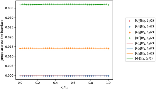
Figure 4. Jumps of the displacement field and the electric potential across the interface on a line along the x1 axis, with ε/h = 0.1.
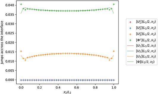
Figure 5. Jumps of the displacement field and the electric potential across the interface on a line along the x2 axis, with ε/h = 0.1.
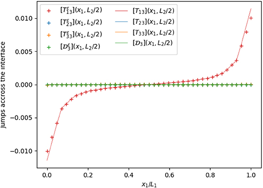
Figure 6. Jumps of the traction vector and normal electric displacement across the interface on a line along the x1 axis, with ε/h = 0.1.
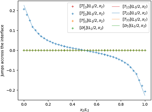
Figure 7. Jumps of the traction vector and normal electric displacement across the interface on a line along the x2 axis, with ε/h = 0.1.
3.1.2. Numerical Results: The Applied Surface Loads
In this section, we study the case of a constant surface load equal to p = 1Pa, applied on the top face of the plate, with no electrical loadings (see Figure 1). The composite laminated plate behaves as a sensor. As previously shown, the numerical results for the unknowns are provided using the dimensionless units. For an applied pressure p, we set:
where and C00 = 1GPa.
In Figure 8 one can observe, as before, that the rate of convergence of the solution of the approximated interface problem to the solution of the initial three phases problem is of order 3. As a consequence, even if the relative thickness of the interphase is large, the asymptotic approximation provides accurate results. More precisely, in the case of a relative thickness of the interphase equal to 0.1, the relative difference is equal to 0.07% for the displacement field and is equal to 0.1% for the electric potential.
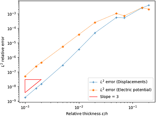
Figure 8. Convergence results with respect to the relative thickness ε/h.
Figure 9 presents the trend of the displacement field and electric potential on the orthogonal line to the interface mid-plane defined by (x = L1/2, y = L2/2, z/h ∈ [−0.5, 0.5]), showing a good numerical fit between the three-phases problem solution (solid line) and our generalized interface model solution (dotted line). As expected, the composite laminated plate, being more elongated on the x1 axis, shows a Kirchhoff–Love kinematics with respect to U1, while the displacement U2 almost vanishes along the fiber. The electric potential presents a quadratic trend which coherent with the results proposed in Fernades and Pouget (2002). Moreover, since the PZT-4 adhesive layer is much more stiffer and has higher electric conductivity with respect to the PVDF adherents, it behaves as a rigid highly conducting interface, as shown in Figures 10–13, according to which the jump of the piezoelectric state almost vanishes at the interface, while the jump of the traction vector can be different from zero (see [T33]).
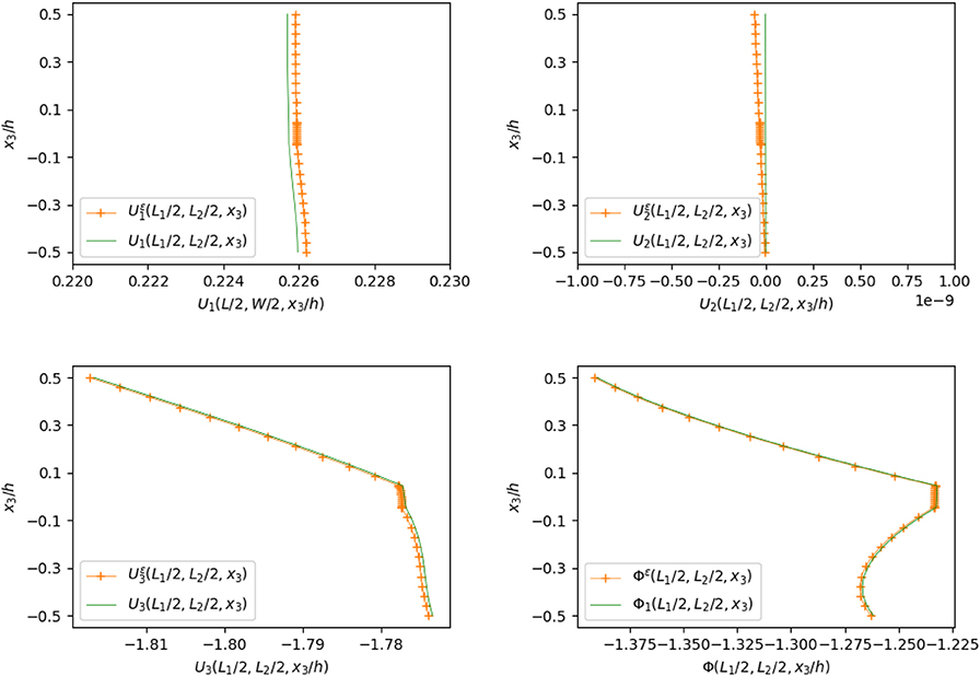
Figure 9. Displacement field and electric potential on a section along the x3 axis, with ε/h = 0.1.
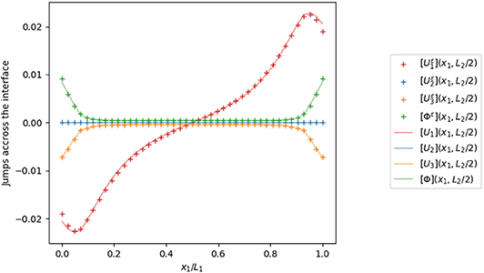
Figure 10. Jumps of the displacement field and the electric potential across the interface on a line along the x1 axis, with ε/h = 0.1.
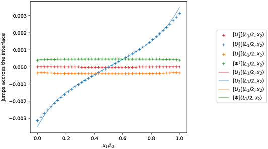
Figure 11. Jumps of the displacement field and the electric potential across the interface on a line along the x2 axis, with ε/h = 0.1.
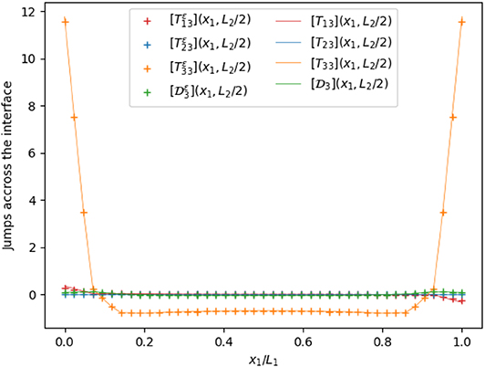
Figure 12. Jumps of the traction vector and normal electric displacement across the interface on a line along the x1 axis, with ε/h = 0.1.
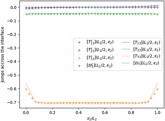
Figure 13. Jumps of the traction vector and normal electric displacement across the interface on a line along the x2 axis, with ε/h = 0.1.
3.2. The Thermo-Elastic Case
The interface problem (6) can be easily adapted in the case of linear elasticity with thermal effect. The thermo-elastic state is defined by the pair s = (u, θ), constituted by the displacement field u = (ui) and the variation of temperature θ: = T − T0, where T and T0 denote the temperature field and a reference temperature, respectively. The corresponding constitutive law takes the following form:
where q = (qi) denotes the thermal flow, X = (Xij) and K = (Kij) represent, respectively, the thermal expansion tensor and the thermal conductivity tensor.
Adapting the same method used for the case of piezoelectricity, the variational problem for thermo-elasticity can be easily derived, where the bilinear form defined on the interface S is given by
where v denotes the displacement test function and .
In what follows, we consider the same geometrical setting of Figure 1, namely a thermo-elastic laminated plate occupying a 3D domain defined by Ω = [0, L1] × [0, L2] × [−h/2, h/2], with L1 = 10h and L2 = 5h. The boundary and loading conditions are slightly different with respect to the piezoelectric cases. We suppose that:
• The union of the lateral boundaries Γ1 is a free boundary;
• A portion of (or the whole) top face Γ2 is subject to a variation of temperature θ1 = 1 K around a given temperature T0 and is mechanically free;
• The bottom face Γ3 is vertically clamped and subject to a variation of temperature θ = 0 K around a given temperature T0;
• No mechanical volume or surface loads are applied.
The reference temperature T0 is set at 310 K. We assume that both the adherents and the adhesive are made of thermo-elastic isotropic materials, such that , Kij = kδij, Xij = βδij, where δij represents the Kronecker's delta. The constitutive coefficients are defined in Table 2:
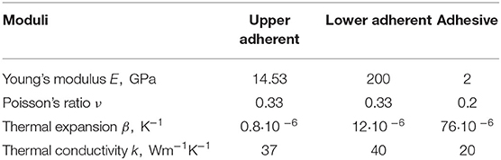
Table 2. Thermo-elastic material properties.
Remark. These data comes from Rakotomanana and Ramaniraka (2004), devoted to the bonding of metallic implant on bones using cement. The upper body models the bone, the lower body represents the metallic implant, while the adhesive is made of classical cement used in this type of surgery. Let us notice that the rigidity of the interphase is very smaller than the rigidity of the implant (the ratio between the Young's modulus is equal to 1%). In that case, the displacements in the interphase is large compared to the displacements in the adherents. This case is generally called a soft interface problem, and it is often considered that the rigidity of the interphase depends linearly of the thickness in the asymptotic analysis (see, e.g., Dumont et al., 2018). It is worth noticing that in the present work the interphase is considered as a hard interface.
3.2.1. Numerical Results: The Applied Variation of Temperature
In all the numerical simulations, the problem is treated as a full coupled problem, with a variable s = (u, θ) with values in ℝ4. The Finite Elements are piecewise linear on thetrahedrons (commonly called P1 Finite Elements). The number of nodes of the mesh is equal to 5824 (resp. 6552) for the interface problem (resp. the three phases problem), leading to 24,275 (resp. 27,187) degrees of freedom. In this case, we did not use dimensionless unit.
In Figure 14 is shown the trend of convergence of the solution of the interface problem to the solution of the three phases problem. Even in the less favorable case of a relative thickness ε/h of 10−1, corresponding to comparable thickness for the adhesive and the adherents, the relative L2 error is below 1% for the displacement field and 10−2% for the temperature field.
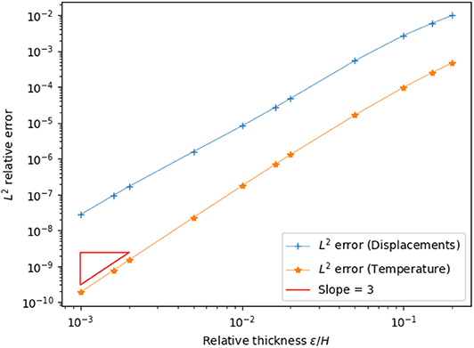
Figure 14. Convergence with respect to the relative thickness ε/h.
In Figure 15 is reported the displacement and temperature fields on a section along the x3 axis for a relative thickness of the interphase equal to 0.04. Continuous curves correspond to the numerical solution of the original three-dimensional problem, while the dotted curves to the data calculated by numerically implementing the transmission conditions. We obtain a relative difference of 0.06% in terms of displacement, and of 9 · 10−4% in terms of temperatures. The applied temperature difference between the upper and lower faces provides an elongation along x3 of the composite. The adhesive layer is characterized by weaker elastic material properties with respect to the adherents, while the thermal conductivities are slightly similar (see Table 2). Thus the interphase behaves as a soft interface from the mechanical point of view and almost hard interface in terms of the heat conduction, providing a jump on the displacement field and a quasi-constant temperature variation across the interface.
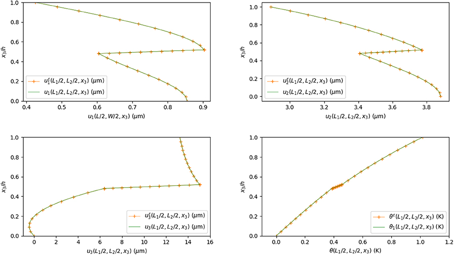
Figure 15. Displacement field and temperature on a section along the x3 axis, with ε/h = 0.04.
In Figures 16, 17, we present the jumps of the displacement, temperature, traction vector and normal heat flow across the interface on a line along the x1 axis. Even if the jumps are large relatively to the displacements and the temperatures, one can conclude that the interface approximation is able to correctly reproduce their distributions. The soft elastic interface behavior is also corroborated by the vanishing of the traction vector jump, which is typical of weak interface models.
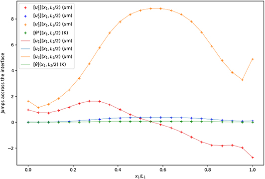
Figure 16. Jumps of the displacement field, temperature (left), traction vector, and thermal flux (right) across the interface on a line along the x1 axis, with ε/h = 0.04.
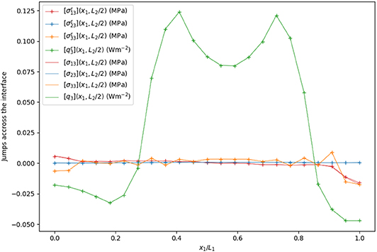
Figure 17. Jumps of the displacement field, temperature (left), traction vector, and thermal flux (right) across the interface on a line along the x1 axis, with ε/h = 0.04.
4. Conclusions
The validity of multiphysic interface transmission conditions as an approximated model of a thin multiphysic thin layer has been discussed through numerical examples. The investigation has be framed within the context of two different multiphysical context: piezoelectricity and thermo-mechanical coupling. The numerical simulation have been developed by using a finite element approach which generalizes an analogous methodology already proposed in Dumont et al. (2018) in the framework of linearized elasticity. In the numerical examples, a composite made of two phases joined by an adhesive has been studied in two different configurations. In the first configuration, the adhesive is a three-dimensional thin endowed with material parameters taken to be softer or harder than the material parameters of the two adherents. In the second configuration, the adhesive is a material interface, whose transmission conditions are the multiphysic interface laws obtained in Serpilli et al. (2019). The relevant fields of the two configurations (displacement, electric potential, temperature) are then compared to test the validity of the proposed interface laws. The latter have been obtained for several cases of material behavior of the adhesive: soft, hard and rigid. These case are numerically compared with the three-dimensional solution (the first configuration). A good agreement has been found even if the elastic moduli of some layers of the adhesive are of the same order as that of the adherents. Moreover, we show that the rate of convergence of the L2-relative error of the current model increases when compared to the one obtained with two classical interface models, namely the hard and soft interfaces. These findings clearly indicate that the approach of substituting the multiphysic interphase with the proposed interface law provides a robust modeling for the composite and improves the numerical results with respect to classical interface laws. This fact, intuitive but not a priori obvious, represents the main original result of the present paper.
Data Availability Statement
The datasets generated for this study are available on request to the corresponding author.
Author Contributions
SD: numerical analysis. MS and RR: asymptotic theory. FL: mechanical modeling.
Conflict of Interest
The authors declare that the research was conducted in the absence of any commercial or financial relationships that could be construed as a potential conflict of interest.
References
Benveniste, Y., and Miloh, T. (2001). Imperfect soft and stiff interfaces in two-dimensional elasticity. Mech. Mater. 33, 309–323. doi: 10.1016/S0167-6636(01)00055-2
Bessoud, A.-L., Krasucki, F., and Serpilli, M. (2011). Asymptotic analysis of shell-like inclusions with high rigidity. J. Elastic. 103, 153–172. doi: 10.1007/s10659-010-9278-1
Bonetti, E., Bonfanti, G., Lebon, F., and Rizzoni, R. (2017). A model of imperfect interface with damage. Meccanica 52, 1911–1922. doi: 10.1007/s11012-016-0520-1
Bonnet, M., Burel, A., Duruflé, M., and Joly, P. (2016). Effective transmission conditions for thin-layer transmission problems in elastodynamics. The case of a planar layer model. ESAIM: M2AN 50, 43–75. doi: 10.1051/m2an/2015030
Dumont, S., Rizzoni, R., Lebon, F., and Sacco, E. (2018). Soft and hard interface models for bonded elements. Composit. B Eng. 153, 480–490. doi: 10.1016/j.compositesb.2018.08.076
Fernades, A., and Pouget, J. (2002). An accurate modelling of piezoelectric multi-layer plates. Eur. J. Mech. A Solids 21, 629–651. doi: 10.1016/S0997-7538(02)01224-X
Fouchal, F., Lebon, F., and Titeux, I. (2009). Contribution to the modelling of interfaces in masonry construction. Construct. Build. Mater. 23, 2428–2441. doi: 10.1016/j.conbuildmat.2008.10.011
Geis, W., Mishuris, G., and Sandig, A. (2004). Asymptotic Models for Piezoelectric Stack Actuators With Thin Metal Inclusions. Berichte aus dem Institut fur Angewandte Analysis und Numerische Simulation 2004/001, Preprint IANS.
Geuzaine, C., and Remacle, J.-F. (2009). GMSH: a 3-D finite element mesh generator with built-in pre- and post-processing facilities. Int. J. Num. Methods Eng. 79, 1309–1331. doi: 10.1002/nme.2579
Geymonat, G., Hendili, S., Krasucki, F., Serpilli, M., and Vidrascu, M. (2014). “Asymptotic expansions and domain decomposition,” in Domain Decomposition Methods in Science and Engineering XXI. Lecture Notes in Computational Science and Engineering, eds J. Erhel, M. Gander, L. Halpern, G. Pichot, T. Sassi, and O, Widlund (Cham: Springer), 749–758. doi: 10.1007/978-3-319-05789-7_72
Geymonat, G., Krasucki, F., and Lenci, S. (1999). Mathematical analysis of a bonded joint with a soft thin adhesive. Math. Mech. Solids 16, 201–225. doi: 10.1177/108128659900400204
Gu, S. T., and He, Q. C. (2011). Interfacial discontinuity relations for coupled multifield phenomena and their application to the modeling of thin interphases as imperfect interfaces. J. Mech. Phys. Solids 59, 1413–1426. doi: 10.1016/j.jmps.2011.04.004
Gu, S. T., Liu, J.-T., and He, Q. C. (2014). The strong and weak forms of a general imperfect interface model for linear coupled multifield phenomena. Int. J. Eng. Sci. 85, 31–46. doi: 10.1016/j.ijengsci.2014.07.007
Hashin, Z. (2002). Thin interphase/imperfect interface in elasticity with application to coated fiber composites. J. Mech. Phys. Solids 50, 2509–2537. doi: 10.1016/S0022-5096(02)00050-9
Javili, A., Kaessmair, S., and Steinmann, P. (2014). General imperfect interfaces. Comput. Methods Appl. Mech. Eng. 275, 76–97. doi: 10.1016/j.cma.2014.02.022
Klarbring, A. (1991). Derivation of a model of adhesively bonded joints by the asymptotic expansion method. Int. J. Eng. Sci. 29, 493–512. doi: 10.1016/0020-7225(91)90090-P
Lebon, F., and Rizzoni, R. (2010). Asymptotic analysis of a thin interface: the case involving similar rigidity. Int. J. Eng. Sci. 48, 473–486. doi: 10.1016/j.ijengsci.2009.12.001
Lebon, F., and Rizzoni, R. (2011). Asymptotic behavior of a hard thin linear interphase: an energy approach. Int. J. Solids Struct. 48, 441–449. doi: 10.1016/j.ijsolstr.2010.10.006
Lotfi, H., and Shing, P. (1994). Interface model applied to fracture of masonry structures. J. Struct. Eng. 120, 63–80. doi: 10.1061/(ASCE)0733-9445(1994)120:1(63)
Lourenço, P., and Rots, J. (1997). Multisurface interface model for analysis of masonry structures. J. Eng. Mech. 123, 660–668. doi: 10.1061/(ASCE)0733-9399(1997)123:7(660)
Mariano, P. (2002). Multifield theories in mechanics of solids. Adv. Appl. Mech. 38, 1–93. doi: 10.1016/S0065-2156(02)80102-8
Raffa, M., Lebon, F., and Rizzoni, R. (2018). Derivation of a model of imperfect interface with finite strains and damage by asymptotic techniques: an application to masonry structures. Meccanica 53, 1645–1660. doi: 10.1007/s11012-017-0765-3
Rakotomanana, L. R., and Ramaniraka, N. A. (2004). “Thermomechanics of bone-implant interfaces after cemented joint arthroplasty: theoretical models and computational aspects,” in Computational Bioengineering, eds M. Cerrolaza, G. Martinez, M. Doblare, and B. Calvo (London: Imperial College Press), 185–214. doi: 10.1142/9781860945403_0009
Renard, Y., and Pommier, J. (2002). GetFem++. An Open Source Generic c++ Library for Finite Element Methods. Technical report, INSA, Lyon.
Rizzoni, R., Dumont, S., and Lebon, F. (2017). On Saint Venant-Kirchhoff imperfect interfaces. Int. J. Nonlinear Mech. 89, 101–115. doi: 10.1016/j.ijnonlinmec.2016.12.002
Rizzoni, R., Dumont, S., Lebon, F., and Sacco, E. (2014). Higher order model for soft and hard elastic interfaces. Int. J. Solids Struct. 51, 4137–4148. doi: 10.1016/j.ijsolstr.2014.08.005
Serpilli, M. (2015). Mathematical modeling of weak and strong piezoelectric interfaces. J. Elastic. 121, 235–254. doi: 10.1007/s10659-015-9526-5
Serpilli, M. (2017). Asymptotic interface models in magneto-electro-thermo-elastic composites. Meccanica 52, 1407–1424. doi: 10.1007/s11012-016-0481-4
Serpilli, M. (2018). On modeling interfaces in linear micropolar composites. Math. Mech. Solids 23, 667–685. doi: 10.1177/1081286517692391
Serpilli, M. (2019). Classical and higher order interface conditions in poroelasticity. Ann. Solid Struct. Mech. 11, 1–10. doi: 10.1007/s12356-019-00052-5
Serpilli, M., and Lenci, S. (2012). Asymptotic modelling of the linear dynamics of laminated beams. Int. J. Solids Struct. 49, 1147–1157. doi: 10.1016/j.ijsolstr.2012.01.012
Serpilli, M., and Lenci, S. (2016). An overview of different asymptotic models for anisotropic three-layer plates with soft adhesive. Int. J. Solids Struct. 81, 130–140. doi: 10.1016/j.ijsolstr.2015.11.020
Keywords: asymptotic analysis, interfaces, multiphysic materials, numerical analysis, finite element analysis
Citation: Dumont S, Serpilli M, Rizzoni R and Lebon FC (2020) Numerical Validation of Multiphysic Imperfect Interfaces Models. Front. Mater. 7:158. doi: 10.3389/fmats.2020.00158
Received: 06 December 2019; Accepted: 04 May 2020;
Published: 05 June 2020.
Edited by:
Chiu Tai Law, University of Wisconsin-Milwaukee, United StatesReviewed by:
Xiaowei Zeng, University of Texas at San Antonio, United StatesAlberto Salvadori, University of Brescia, Italy
Copyright © 2020 Dumont, Serpilli, Rizzoni and Lebon. This is an open-access article distributed under the terms of the Creative Commons Attribution License (CC BY). The use, distribution or reproduction in other forums is permitted, provided the original author(s) and the copyright owner(s) are credited and that the original publication in this journal is cited, in accordance with accepted academic practice. No use, distribution or reproduction is permitted which does not comply with these terms.
*Correspondence: Serge Dumont, serge.dumont@unimes.fr