An Efficient Track-Scale Model for Laser Powder Bed Fusion Additive Manufacturing: Part 1- Thermal Model

Introduction

Laser powder bed fusion (LPBF) is an additive manufacturing (AM) process where a laser is used to locally consolidate powder into a desired geometry. Development of LPBF parts generally requires expensive trial-and-error experiments to determine an ideal set of laser parameters. A finite element (FE) model could be used to determine a set of laser parameters to reduce the number of defects and experimental iterations required to produce a functional AM part (Bikas, Stavropoulos, and Chryssolouris 2016; Tangestani et al., 2020).

Modeling requires knowledge of the material’s thermo-mechanical behavior at different length scales. For LBPF processes, the laser spot size ranges from 50 to 250 µm (Yin et al., 2012; Paul, Gupta, and Singh 2015; Irwin and Michaleris 2016), while the final parts can achieve sizes in the centimeter scale. Consequently, to simulate full-scale AM parts, FE models must have large model sizes and high computational costs (Yang et al., 2018). There are limited publications describing a functional multi-scale model in detail and even fewer papers predicting the temperature field in a part-scale model (Pal et al., 2014; Francois et al., 2017; Liang et al., 2018; Gouge et al., 2019).

To simulate the thermal history and melt pool geometry, it is essential to accurately model the laser heat source. Depending on the length scale of the simulation, there are different types of heat input models such as beam-scale, track-scale, and layer-scale heat input models (Gouge et al., 2019). One common approach to model laser melting at the part scale (macroscopic) is the lumped laser model where the heat source is distributed over multiple build layers. Several publications have applied a lumped heat source approach to LPBF simulation (King et al., 2015; Hodge, Ferencz, and Vignes 2016; Yang et al., 2018). This can accurately predict the part distortion and residual stresses but lacks resolution for thermal history at micro- and macroscopic scale. Beam-scale heat input models are capable of predicting the melt pool geometries, temperature distributions, and phase transitions within LPBF-printed parts as demonstrated in (Mukherjee, Zhang, and DebRoy 2017; Cook and Murphy 2019). However, to solve a typical transient beam-scale model, finite elements and time increments must be in the range of 100,000 and over 1,000,000, respectively, resulting in long computational times rendering it impractical at the part scale (Irwin and Michaleris 2016). To successfully model the effect of the laser beam at multiple scales, a model accounting for the effect of the laser beam at a larger scale must be developed.

One conventional approach to decrease the computational time at the laser-beam scale (microscopic) is to average the heat input over its path and simulate an entire track length in one increment. This is possible due to the high laser scan speed of the LPBF process. Luo and Zhao consider a simple Gaussian 2D track-scale heat source for a thermal model, which decreases the computational time by 70% (Luo and Zhao 2019). However, a 3D heat input is required to accurately simulate the heat penetration within the powder (Gusarov et al., 2009) and the heat distribution under the laser beam is far from a simple circular shape. Irwin and Michaleris propose a 3D heat source model to reduce the computational time by a factor of 100 with 10% error in predicted distortion (Irwin and Michaleris 2016). The model developed by Irwin and Michaleris (Irwin and Michaleris 2016) simulates the entire Goldak et al. heat input (Goldak, Chakravarti, and Bibby 1984) as a single heat input calculation. The semi-ellipsoidal power distribution proposed by Goldak et al. (Goldak, Chakravarti, and Bibby 1984) was originally developed for welding processes. Recently, Liu et al. (Liu et al., 2018) developed a new equation to describe the LPBF heat source more accurately. It follows a Gaussian profile on the Cartesian coordinate system, and an exponentially decaying profile along the z-direction. Zhang et al. (Zhang et al., 2019) showed that the exponentially decaying (ED) heat source model replicates the rapidly-moving LPBF laser heat source better than the model developed by Goldak et al.

Besides the laser heat source, the effect of the powder on heat absorption and cooling of the consolidated material must be considered during modelling of LPBF processing. The Irwin and Michaleris model neglects the effects of the powder state on the heat transfer boundary conditions (Irwin and Michaleris 2016). The powder properties have a significant effect on the LPBF thermo-mechanical performance, which has been described in (Li et al., 2019). Sih and Barlow (Sih and Barlow 1994) showed thermal conductivity of the powder is significantly lower than the solid state of the material, which influences the heat distribution and residual stress.

In this series, a new track-scale model is proposed to account for the thermo-mechanical behavior at the microscopic scale. A new Hybrid Line (HL) heat input model is derived from the 3D ED heat input model from (Liu et al., 2018). The model accounts for the material state transition from powder to solid. It is calibrated for high gamma prime nickel-based (Ni-based) superalloys by incorporating thermo-mechanical properties of the powder and fully dense material. The first part of this work focuses on simulating the thermal behavior of LPBF. The HL model is evaluated by comparing the processing time and thermal behavior to experimental results and single-track simulation using beam scale ED model. Predicted melt pool geometries, nodal temperatures, cooling rates and temperature distributions are evaluated.

Material and Experimental Method

Material Composition

In this study, a gas-atomized high-γ’ Ni-based superalloy RENÉ 65 (R65) powder, produced by ATI Powder Metals, is used. Ni-based superalloys are commonly used for high-temperature applications such as turbine blades and compressor vanes in aircraft gas turbine engines (Thatte et al., 2016; Thatte, Martin, and Hanlon 2017; Stinville et al., 2018). The powder particles were mostly spherical with a size distribution of 12–42 µm. The R65 chemical composition is 15%, Cr, 13% Co., 4% W, 4% Mo, 3.5% Ti, 2.1% Al, 0.9% Fe, 0.7% Nb, 0.05% Zr, 0.04% Ta, 0.01% B and the balance is Ni.

LPBF Experimental Procedure

To validate the HL model, a single-track LPBF design of experiments (DOE) was completed. The DOE print was conducted on an Aconity MIDI LPBF machine under atmospheric pressure conditions. A 120 mm × 85 mm × 2 mm substrate was printed on a non-pre-heated circular steel base plate using the as-received R65 powder. The as-built substrate was extracted and polished to minimize the surface roughness before printing a series of single tracks. A total of 90 single tracks were printed using 18 different process parameter combinations in a 40-μm thick powder layer on the polished substrate. Each set of parameters was repeated five times to achieve statistically consistent results. The process parameters investigated in this DOE included laser power and laser speed. The laser speed was varied from 800 to 1,300 mm/s in increments of 100 mm/s, and the laser power was varied from 180 to 220 W in increments of 20 W. The single-track DOE is shown in Figure 1A. A laser beam radius of 60 μm was maintained for the printing process.

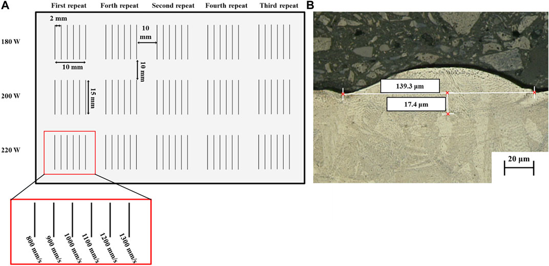
FIGURE 1. (A) Single track DOE parameters and configuration on the powder bed substrate. (B) Optical microscope image showing R65 single track melt pool produced by LPBF with a laser speed of 800 mm/s and power of 200 W.

Melt Pool Characterization

The printed single-track experiments were cross-sectioned perpendicular to the laser-path. Each block was mounted, ground and polished using standard metallographic techniques, then etched for 30 s with Glyceregia (15 ml HCl, 10 ml Glycerol, 5 ml HNO3). Optical microscopy using a Keyence VK-X250 confocal laser microscope was completed to measure the melt pool width and depth of the printed tracks. Figure 1B shows an example of the melt pool dimensions obtained using this approach. The penetration into the substrate is considered the depth, and the distance between two edges of the melted zone is considered the width of the melt pool.

Modelling of the Laser Heat Source

Accurate simulation of the LPBF process requires a thermal model capable of reproducing the laser heat input together with the dynamic phase transition between the solidified part and the powder bed. This section first describes the well-established beam-scale ED model used as a reference. Secondly, the new track-scale 3D heat source model developed for LPBF is described. Finally, the heat dissipation and FE implementation methodology are provided.

Beam Scale Exponentially Decaying Heat Input Model

In the ED model, the heat input energy from the laser is represented as a Gaussian distribution heat source on the surface and absorbed exponentially through the powder depth. The energy input ($Q$) of the ED model is given by:

where $Q$ is the input energy, $\eta$ is the absorption coefficient, and $P$ is the laser power. The parameters $x$, $y$, and $z$ represent the orientations of the local coordinates, $r_l$ is the radius of the laser, and $q_0$ is the value of a 2D Gaussian heat input profile. The energy penetration depth within the powder is computed using the coefficient $H$, equal to the powder layer thickness, as done in (Liu et al., 2018).

Track Scale Hybrid Line Heat Input Model

For the HL model, the energy from the ED heat input model given in Eq. 1 is integrated over a time increment using Eq. 2:

where $\Delta t$ is the time increment, $t_0$ is the time at the beginning of the increment and $\overline{Q}$ is the time-average of the beam-scale heat input model. By substituting Eq. 1 into Eq. 2, the moving HL heat input model in the $x$ direction corresponding to the laser scanning direction becomes:

The function erf is the error function while $x_{start}$ and $x_{end}$are the spatial start and endpoints of the heat input model. These two variables are defined by the laser speed ($v_s$) and time increment ($\Delta t$). The parameter $\eta$ is the absorption factor obtained from (Keller et al., 2017), and the coefficient $C$ is calibrated to match the ED model and account for the effect of latent heat. The track-scale model is more computationally efficient than the beam-scale model due to the increased time increment $\Delta t$, allowing fewer computations over the same track length. The time increment is dictated by the displacement equation $\left(\Delta x=v_s\Delta t\right)$ and the terminal points $\left(x_{start},x_{end}\right)$ of the scanned laser track.

Implementation of Heat Dissipation

The standard equations (Newton’s laws) for heat dissipation during LPBF are taken from (Pham and Dimov 2001) and are applied to the two models. The equations developed by Sih and Barlow (Sih and Barlow 1994) are used to simulate the energy loss due to radiation. The overall emissivity is expressed as:

and

where $\varphi$ is the powder bed relative density (65% from the machine settings), ${\epsilon }_s$ is the emissivity of the solid (0.22) (Kieruj, Przestacki, and Chwalczuk 2016), ${\epsilon }_H$ is the emissivity between adjacent powder particles, and $A_H$ is the area fraction of pores. Open surfaces are accounted for using convective boundary conditions based on the work of Li et al. (2019), and a value of 20 $\left(\frac{W}{m^{2 o}C}\right)$ is used as the coefficient for uniform natural convection. The ambient and initial temperatures for the model are both set to room temperature, 25°C.

Model Implementation in Finite Elements

The two heat transfer models (ED and HL) are implemented in Abaqus, a commercial finite element software. A part domain of 2.0 × 0.5 × 1.0 mm is modelled to capture melt pool dimensions of the beam- and track-scale models, as shown in Figure 2. The domain dimensions are selected to ensure a stable melt pool during the simulation as studied in (Cheng and Chou 2015). The powder layer thickness implemented in the model is 0.04 mm based on LPBF settings described in Laser Powder Bed Fusion Experimental Procedure. DC3D8 elements are used to mesh the substrate and powder layer. Based on a mesh sensitivity study, the powder region interacting with the laser is meshed with element dimensions of 10 μm for the $y$ and $z$ directions, and 20 μm for the $x$-direction. Coarser elements are employed for regions further from the laser heat source to decrease computation time.

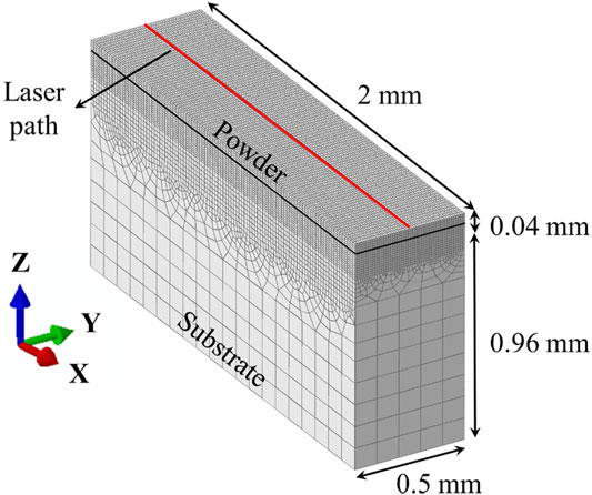
FIGURE 2. Meshed 3D model for the FE simulations. The powder layer and substrate are 0.04 and 0.96 mm thick, respectively. Mesh sizes for the powder are finer (10 µm) compared to the substrate to increase computational efficiency. The red line along the X direction shows the laser path where the nodal temperatures are evaluated.

Material Properties

Temperature-dependent material properties such as specific heat capacity and thermal conductivity are used in the solid substrate and R65 powder, as demonstrated in Figure 3. The thermal conductivity was experimentally measured using the laser flash approach described in (Touloukian, 1970), and the specific heat capacity was measured by pulse heating and enthalpy methods from (Touloukian and Buyco 1970). For the track-scale model, modified specific heat data is used to avoid failure in convergence. There is a spike in specific heat capacity around 1,000°C in Figure 3A that could generate numerical instabilities. A line extended from the last point before the peak and a “cut-off temperature” of 1,100°C is used to modify the data, as done in (Promoppatum and Rollett 2021). This is necessary for Ni-based superalloys due to gamma prime phase transformation, resembling the approaches used in (Baykasoglu et al., 2018; Olleak and Xi 2018; Anca et al., 2011; Rahman et al., 2019) for superalloys. However, this may not be required for the model’s application to other alloy systems depending on the specific heat capacity as a function of temperature. The heat conduction coefficient inside the melt pool is set 2.8 times higher than solid-state to compensate for the convective heat transfer due to fluid flow inside the melt pool (see Figure 3B) (Ding 2012). The liquid state is not considered in the model, but a higher thermal conductivity is used for nodal temperatures above the liquidus. The liquidus (1,381°C) and solidus (1,338°C) were obtained experimentally using differential scanning calorimetry (DSC).

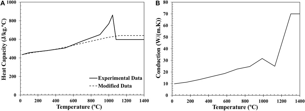
FIGURE 3. (A) Experimental and modified temperature-dependent specific heat capacity and (B) heat conduction as a function of temperature for R65.

For the powder bed, the effective thermal conductivity k is taken from (Sih and Barlow 1994; Kundakcıoğlu et al., 2018) and is defined as:

where $k_s$ is the solid material thermal conductivity, $k_f$ is the thermal conductivity of air, and $k_r$ represents the thermal conductivity portion of the powder bed. The coefficient $k_r$ accounts for radiation among particles, as described in the following equation taken from (Kundakcıoğlu et al., 2018):

where $d_p$ is the powder particle diameter. A value of 8,276 kg/m³ provided by the material supplier is used for the powder density and the following equation is used to determine the powder state density:

where ${\rho }_p$ is the powder bed density and ${\rho }_s$ is the density of the fully dense material.

The latent heat of melting (247,075 J), obtained experimentally using DSC, is taken into consideration in the ED model but not in the track-scale model. This is because of the convergence issue described previously. The latent heat of evaporation is assumed to be 33 times larger than the melting energy based on (Cao and Yuan 2019) who used a similar alloy. The temperature range of the phase transformation for evaporation is assumed to be from 3,000°C to 3,500°C; however, these temperatures are not approached in the track-scale simulations.

Modelling Material State Transformation

During LPBF processing, the material undergoes phase changes from solid powder to a liquid in the melt pool and back to a consolidated solid material. The liquid phase of the material is modelled as solid state with higher conduction as explained in Material properties. Both FEM implementations (ED and HL models) account for the material state changes. Above the melting temperature, the powder to solid-state transition is incorporated within the model using the USDFLD subroutine code in Abaqus. The relative density of the material state is stored in an index as shown in the legend of Figure 4A. The powder value is 0.65 (shown in blue), while the consolidated solid and liquid states both have a value of 1 (shown in red). The nodal temperature and the region experiencing temperatures higher than the melting point are shown in Figure 4B. Comparison of the figures demonstrates the correlation of the material transition and the nodal temperature during the process.

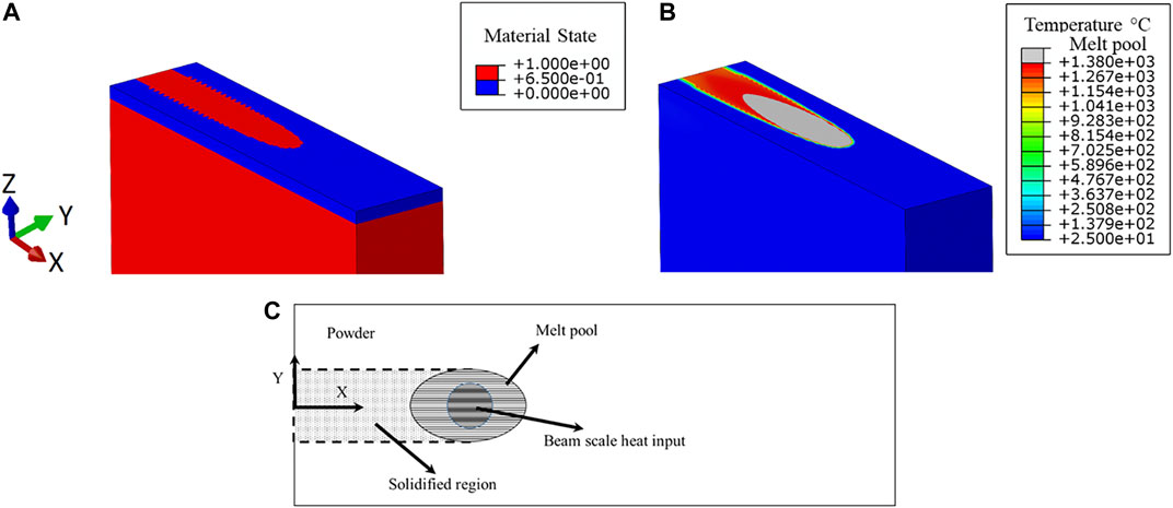
FIGURE 4. ED model simulation showing the material state transition and temperature distribution. In (A), the powder (blue) and liquid/solid (red) zones are shown. (B) Nodal temperature during the process. In (C), a schematic of the material state transition occurring in the melt pool is shown.

The USDFLD subroutine is called at the beginning of every time step to read the material index of each integration point to determine the material state and resulting properties. Figure 4C shows a schematic of the material state changes occurring at the beam scale. The heat source must always remain above the melt pool to accurately predict the material state transition. At time increment n, the DFLUX code applies heat to the material and the solver calculates the nodal temperatures. The material state at the time increment $\text{n}+1$ is obtained from the nodal temperature of the previous increment ($\text{n}$). Consequently, the material state is always one time increment behind the applied heat source. Because the time increment in the ED model is small, the heat source is always situated above the melt pool allowing a low lag in material state transition. However, increasing the time step in the HL model causes significant delay in the material state transition and inaccuracy in thermal simulation, as shown in Figure 5A–D. Figures 5A,B show the nodal temperatures for subsequent time steps. The black ellipsoid shows the location of the applied heat. The lag of one increment between the heat input and the material state can be clearly observed in Figures 5C,D, as the applied heat is one increment in front of the material state transition.

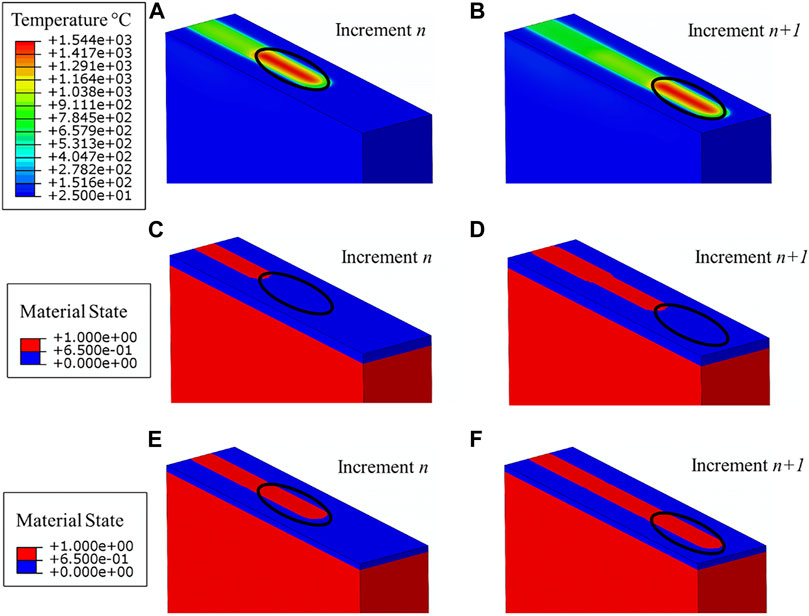
FIGURE 5. Nodal temperatures are shown in increments (A) $\mathbf{n}$ and (B) $\mathbf{n}+1$. The material state transition showing the lag effect in increment (C) $\mathbf{n}$ and (D) $\mathbf{n}+1$. The modified material state transition is shown in increment (E) $\mathbf{n}$ and (F) $\mathbf{n}+1$without lag. Powder state is shown in blue and liquid/solid state is shown in red. The black ellipsoid shows the location of the applied heat.

To overcome any potential issue with the lag in phase transition, a new method accounting for phase transformation is proposed. To resolve the problem presented in Figure 5A–D , the material state change is set to occur above 5% of the total energy absorption for the HL model, as shown in Figures 5E,F. The value of 5% is calculated from the energy required to increase the material temperature to the melting point, which was used to predict the initial temperature of the activated material in (Li et al., 2019). This value might differ slightly for other materials but is not expected to influence the accuracy of the results. The lag of one increment between the heat input and the material state is now eliminated. This approach enables faster convergence of line heat input models and improves the accuracy of the predictions.

Results and Discussion

LPBF Melt Pool Geometry Analysis

Figure 6 shows the measured melt pool dimensions (depth and width) associated with the 18 different line energies described in Figure 1A. Each set of adjacent figures Figure 6A–F shows the melt pool depth and width with identical laser powers for different laser speeds. The error bars represent the maximum and minimum values of the five experimental repeats.

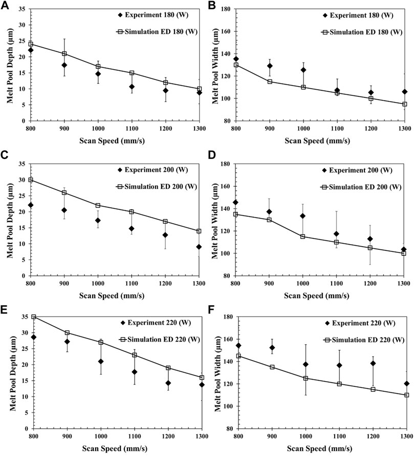
FIGURE 6. Comparison between experimental and ED simulation melt pool widths and depths for different laser powers: (A) and (B) 180 W (C) and (D) 200 W, and (E) and (F) 220 W.

As laser power increases, line energy increases, consequently leading to larger melt pool dimensions. Table 1 shows how the melt pool depths and widths increase at average rates of 16.4 $\frac{\mu m}{W}$ and 54.59 $\frac{\mu m}{W}$ with laser power in Figure 6. Conversely, as the laser speed increases, melt pool depths and widths decrease at average rates of 2.87 $\frac{\mu m}{(mm/s)}$ and 7.13 $\frac{\mu m}{(mm/s)}$, respectively. Therefore, the laser power has more significant effect on the melt pool size than laser speed. Current results are consistent with previous researchers (Fu and Guo 2014; Irwin and Michaleris 2016) who also reported a stronger influence of laser power on the melt pool geometry.

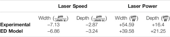
TABLE 1. Comparison of the melt pool depths and widths for the ED models and experiments with increasing laser speed and power.

The melt pool aspect ratio defined as melt pool depth divided by melt pool width shown in Figure 6 are plotted in Figure 7A with respect to the line energy density. The melt pool aspect ratio increases with increasing line energy density. The heat transfer mode generally transitions from conduction to keyhole mode between an aspect ratio of 0.4–0.5 (Ghosh et al., 2018; Cloots, Uggowitzer, and Wegener 2016; Khairallah et al., 2016), above which melt pools are in keyhole mode. Since the aspect ratio falls below 0.2 for each case, all laser conditions evaluated in this study are in conduction mode. The absence of a bell-shaped melt pool for the highest line energy density in Figure 7B confirms that the heat transfer mode is not keyhole. Additional studies would be required to validate the proposed HL model for laser heat sources operating in keyhole mode.

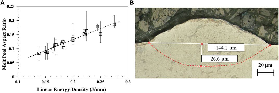
FIGURE 7. (A) Effect of linear energy density (J/mm) on the experimental melt pool aspect ratio (depth over width). (B) Melt pool cross-section obtained with a laser power of 220 W and laser speed of 800 mm/s. The red dashed line outlines the melt pool boundary.

ED Model Evaluation

The laser radius ($r_l$) and $H$ coefficient correspond to the experimental laser beam radius (60 µm) and powder bed thickness (40 µm) as recommended in (Liu et al., 2018). The absorption coefficient ($\eta$) for Ni-Based superalloys is 0.5 as per (Keller et al., 2017).

The ED heat input model is validated with the experimentally measured melt pool dimensions. The method used to measure the simulated melt pool geometry is shown in Figure 8. The grey region represents the area above the liquidus temperature, and only the grey portion within the substrate is considered for melt pool measurement.

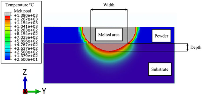
FIGURE 8. Temperature variation surrounding the melt pool for the ED heat input model with 200 W laser power and 1,000 mm/s laser speed. The melted zone is shown in grey, the melt pool in light red, the powder state in blue, and the substrate in dark blue.

The difference between the simulated and measured melt pool depths and widths are shown in Figure 6. Trends on the effect of laser speeds and powers on the melt pool geometries predicted by the ED model match the experimental observations. The simulated melt pool depths and widths increase at average rates of 21.25 $\frac{\mu m}{W}$ and 39.58 $\frac{\mu m}{W}$, respectively, as the laser power increases and decreases at average rates of 3.24 $\frac{\mu m}{(mm/s)}$ and 6.86 $\frac{\mu m}{(mm/s)}$, respectively, when laser speed increases (see Table 1). The predicted melt pool depth and width are on average within 4.2 and 11.0 μm of the experimentally measured values. This lies within the experimental error range derived from melt pool measurement. Henceforth, it can be concluded that the ED model accurately predicts the melt pool geometry.

HL Model Calibration

Following Irwin and Michaleris’s methodology (Irwin and Michaleris 2016), the time increment ($\Delta t$ (s)) of the HL model is normalized over the laser travel distance as follows:

where $v_s$ is laser speed (m/s) and $r_l$ is beam radius (m). The parameter $\tau$ links the laser travel distance with $r_l$. The heat source length of the HL model is equal to the ED beam radius when $\tau =$ 1. When $\tau >$ 1, the heat source length is larger than the ED beam radius, reducing simulation time.

The $H$, $r_l$, and $\eta$ values are maintained from the ED model due to their dependency on the experimental set-up. As the ED model shows good agreement with experimental results, it is used as a reference to calibrate the coefficient $C$ and validate the accuracy of the HL model in terms of temperature distribution and cooling rate. The coefficient $C$ is determined by minimizing the difference in the nodal temperatures in regions surrounding the melt pools between the HL and ED models. A line energy of 200 J/mm is used for calibration and Figure 9 shows where the nodal temperatures are extracted. Cross-sections of the simulation results along the laser track are taken at different times. The number of cross-sections considered in the calibration is varied between three and nine depending on the value of $\tau$ due to the fixed part length. The cross-sections are taken ahead of, inside of and following the laser beam heat source. For each cross-section, only the nodal temperatures outside the melt pool (outside the grey region in Figure 9), are considered for calibration. As the laser heat input is lumped into a line, changing the value of $\tau$ changes the peak temperature in the melt pool. Thus, the temperatures inside the melt pool cannot be used for calibration. The calibration coefficient ($C$) is set to 1.2 independently of the normalized increment time ($\tau$).

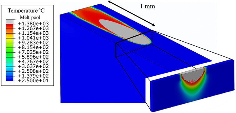
FIGURE 9. Example of an ED laser track simulation used for HL model calibration. The melt pool is shown in grey color. The nodal temperatures of the elements surrounding the melt pool are used for calibration of the HL model. The highlighted region (red cube) at the center of the cross section at the melt pool boundary is used to study the cooling rate in Cooling rate.

Hybrid Line Model Evaluation

Computational Efficiency

The time required to solve the model is dependent on the number of time increments and iterations for each increment. While the term $\tau$ has a linear relationship with the time increment size, the number of iterations required for convergence increases with a larger time increment. Figure 10 shows the ratio between the time required to solve the HL and ED models $\left(\frac{Tim{e}_{ED}}{Tim{e}_{HL}}\right)$. The HL model is 330–1,500 times faster than the ED model as $\tau$ increases from 5 to 20. Even though the ratio should be close to $\tau$ (based on Eq. 3 and Eq.10), it is significantly larger in Figure 10. This is because the heat capacity relationship with temperature is simplified in the HL model and the latent heat is not considered as explained in Material properties. Consequently, the simulation requires a reduction of the time increment size by an average of $\Delta t=7\times {10}^{-7}$ (for ED model) to overcome the convergence issue created by a sudden change in specific heat capacity shown in Figure 3A. The higher computational efficiency of the HL model over the ED model is thus due to simplified material properties and the integrated heat input equation.

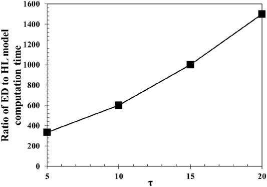
FIGURE 10. Comparison of $\frac{\mathit{Tim}{\mathit{e}}_{\mathit{ED}}}{\mathit{Tim}{\mathit{e}}_{\mathit{HL}}}$ as a function of $\mathit{\tau }$ showing the computational efficiency of the HL model compared to the ED model.

Melt Pool Geometry

The heat input energy in the HL model is simplified from the ED model resulting in inaccuracies in prediction of the melt pool geometry. Nevertheless, the HL model with small time integration step ($\tau =$ 5) offers reasonably accurate results while being 330 times faster than the ED model. Figure 11 shows the predicted melt pool dimensions (depth and width) for the HL model with $\tau =$ 5. The trends on the effect of laser speeds on the melt pool depths predicted by the HL model match the experimental observations. As the laser speed increases, the melt pool width and depth decrease by average rates of 8.29 $\frac{\mu m}{(mm/s)}$ and 3.54 $\frac{\mu m}{(mm/s)}$, respectively. The predicted melt pool depth and width are on average within 5.4 and 27.2 μm of the experimentally measured values. When the integration time step increases above $\tau =$ 5, the simulated melt pool size decreases significantly due to the reduction in peak temperatures.

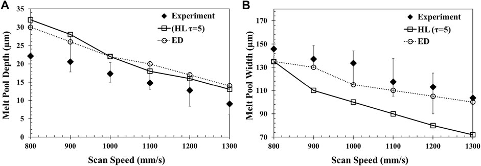
FIGURE 11. Comparison of the experimental and HL simulation ($\mathit{\tau }=$ 5) melt pool (A) depth and (B) width for 200 W laser power.

Laser Track Temperature

Simulation of the laser track temperature is necessary to understand the microscopic material behaviour during LPBF since it has a strong influence on the formation of microstructural inhomogeneity in Ni-based superalloys. This includes formation of bimodal grain structures resulting in strong thermo-mechanical anisotropy of the as-produced specimens discussed in (Carter, Attallah, and Reed 2012; Kontis et al., 2019). Detrimental phases and micro-segregation can arise during the LPBF process, promoting micro-cracking and low part ductility (Cloots, Uggowitzer, and Wegener 2016; Carter, 2013).

The nodal temperatures predicted by the ED and HL models are compared in Figure 12. The temperature distributions are taken on the top surface along the laser path, as shown by the red line in Figure 2 when the laser is located at 1.8 mm (90% of the simulation). The temperature distributions are predicted for three lines energies, 275, 200, and 138 J/mm, in Figures 12A–C, respectively.

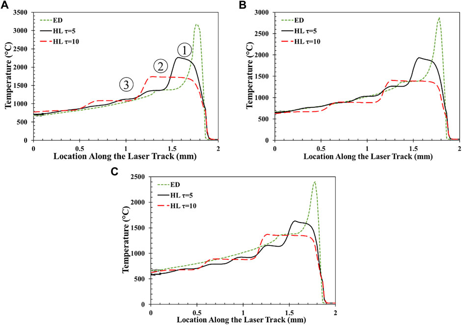
FIGURE 12. Nodal temperatures along laser paths in the ED model and the HL model for $\mathit{\tau }=$ 5 and $\mathit{\tau }=$ 10. The laser powers and speeds are (A) 220 W–800 mm/s (B) 200 W–1,000 mm/s and (C) 180 W–1,300 mm/s.

Both models demonstrate increasing maximum temperature with increasing laser power, consistent with previous experimental observations in (Carter, Attallah, and Reed 2012; Li et al., 2018). However, the HL model fails to capture the maximum temperature under the laser beam location (at 1.8 mm) because the heat input is homogeneously distributed along the time increment. As the $\tau$ value increases, the time step increases, and the maximum temperature decreases when compared with the ED model. The HL model exhibits plateaus in the temperature profiles (see numbers 1, 2 and 3 in Figure 12A). The length of each plateau is proportional to the $\tau$ value and thus to the time step used for integration along the laser path.

As the temperature decreases, the two models start converging in Figure 12 for all laser conditions. The errors in temperature predictions between the two models are given in Table 2 for various temperature ranges. Below 1,400°C, the temperature error varies between 1 and 15% for $\tau =$ 5 and $\tau =$ 10. Between 1,400°C and 1,300°C, the error is only 1.5% for $\tau =$ 10 This is when material solidifies (liquidus = 1,381°C and solidus = 1,338°C). The error is approximately 12% within the solvus temperature range (∼1,110°C (Wessman 2016)). Both temperature ranges are critical to the LPBF of R65 since they are associated with the micro-cracking mechanism often observed in high γ′ Ni-based superalloys (Cloots, Uggowitzer, and Wegener 2016; Carter 2013; Grange et al., 2020) and the formation of carbides and gamma prime (γ’) (Wessman 2016).

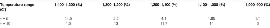
TABLE 2. Error in temperature prediction between ED and HL models for different temperature domains. The laser power and speed are 200 W and 1,000 mm/s, respectively (Figure 12B).

Cooling Rate

The cooling rate controls the thermal gradient causing thermal stresses and strains in the fabricated parts (Li et al., 2018). Therefore, the process-induced cooling rate must be captured accurately during the simulation. A comparison between the cooling rates obtained from the ED and HL models is shown in Figure 13. Three different laser conditions with line energies of 275, 200 and 138 J/mm are compared in Figures 13A–C, respectively. The cooling rates are evaluated at the melt pool boundary central to the laser track because it is a critical region for the formation of residual stresses. This is shown by the red cube element in the cross-section subset in Figure 9. As the melt pool depth depends on the energy input, the results are captured at locations of 40 μm, 22 μm, and 13 µm under the powder layer for line energies of 275, 200, and 138 J/mm, respectively. The maximum cooling rates obtained are on the order of 10⁵ °C/s, one order of magnitude lower than values reported in literature (∼10⁶ °C/s (Wang, Shi, and Liu 2019)). Lower cooling rates are attributed to the extraction of results as the laser reaches the end of the track (2 mm in Figure 2).

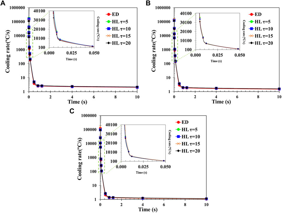
FIGURE 13. Cooling rate profiles for the following laser powers and speeds: (A) 220 W–800 mm/s (B) 200 W–1,000 mm/s, and (C) 180 W–1,300 mm/s.

Figure 13 shows that the cooling rates decrease rapidly and reach steady state around 2°C/s, 1 s after the track is printed. The average errors between the ED and HL models are 5.98, 5.37, 6.86, and 8.2% for $\tau =$ 5, 10, 15, and 20, respectively. Both simulations show that increasing the line energy increases the cooling rate as it increases the maximum nodal temperatures shown in Figure 12. At 1.2 ms, the cooling rate decreases from 2.4$\times$10⁵°C/s to 1.1$\times$10⁵°C/s when the laser power drops from 220 to 180 W.

Temperature Distribution

The simulation of full-scale parts requires the temperature distribution to be accurately simulated. This entails accurate prediction of nodal temperatures, cooling rates, and the heat transfer between the different material states (liquid, solid and powder). Figures 14A,B show the temperature distributions in the ED and HL model with $\tau =$10. The temperature distributions are taken 1.2 ms after track completion to minimize image contour level contrast due to peak temperatures. The nodal temperatures are higher at the end of the track since this is the last location of the laser heat source. The HL model temperature is higher at this position due to the length of its heat source. In both cases, the heat energy is mostly distributed within the solidified region and the substrate. The temperature gradients along the $x$, $y$, and $z$ directions are similar for both models.

FIGURE 14. Temperature distributions captured 1.2 ms after the track simulation finishes for (A) the ED beam scale and (B) the HL track-scale model ($\mathit{\tau }=$ 10).

Conclusion

In this study a new track-scale thermal model referred as the HL heat input model is developed to predict the temperature distribution during the LPBF process. The temperature-dependent specific heat capacity and thermal conductivity are experimentally measured and accounted for in both the ED and HL models. The results of the HL model are evaluated by comparing the predicted temperature distribution, cooling rate and melt pool dimensions to a beam-scale (ED) model and a set of LPBF single track experiments.

The ED beam-scale model was first validated by comparing the predicted melt pool geometry with experimental observations. Results show that the ED model can capture the melt pool geometry within few microns and the trends of the effect of laser speeds on the melt pool geometry within 10% error.

The comparison between the ED and HL models shows that the new track-scale model is a versatile substitute for a beam-scale model. At low $\tau$ value, the model can predict the effect of laser parameters on the melt pool geometry. The predicted melt pool depth deviates by approximately 5 μm, while the width prediction is less accurate due to variation in the peak temperature. The temperature distribution inside the laser path is in good agreement with the beam-scale model. This is specifically true for temperatures below the solidus where the deviation from the ED model remains below 5%. The sub solidus temperature range has the strongest impact on the microstructure generated during LPBF of Ni-based superalloys.

By increasing $\tau$, some of the resolution is lost on the temperature profile resulting in increased error in peak temperature and melt pool geometry prediction. However, the cooling rate, which controls micro- and macroscopic stresses remains below 10% error with respect to the beam scale model. This allows for significant computational gains. At $\tau =$ 5, the HL model is 330 times faster than the ED model and can easily become more than 1,000 times faster by increasing the $\tau$ value. The presented model is beneficial for predicting the in-process temperature field and thermal history that influences the resulting microstructure and mechanical properties of the printed material.

Data Availability Statement

The original contributions presented in the study are included in the article/Supplementary Material, further inquiries can be directed to the corresponding author.

Author Contributions

RT: Developed the track-scale model, evaluated the simulation results, and measured the melt pool dimensions. TS: Contributed with development of the modeling process and helped with writing the paper. AC: Helped experimental part of the paper, measured the melt pools, and contributed to evaluating the keyhole and conduction mode in process. WM: Worked on experimental part of the paper and the design of experiment; and extracted the samples from the baseplate. LY: Printed the single tracks on a single layer of powder and reviewed model development. ÉM: Supervised the project and contributed to writing the paper.

Conflict of Interest

The authors declare that the research was conducted in the absence of any commercial or financial relationships that could be construed as a potential conflict of interest.

Publisher’s Note

All claims expressed in this article are solely those of the authors and do not necessarily represent those of their affiliated organizations, or those of the publisher, the editors, and the reviewers. Any product that may be evaluated in this article, or claim that may be made by its manufacturer, is not guaranteed or endorsed by the publisher.

Acknowledgments

The authors are thankful to Natural Sciences and Engineering Research Council of Canada (NSERC) under Grant Nos. RGPIN-2019-04073. The authors would also like to thank Amber Andreaco, from GE Additive, for supplying the powder material used in this study.

Supplementary Material

The Supplementary Material for this article can be found online at: https://www.frontiersin.org/articles/10.3389/fmats.2021.753040/full#supplementary-material

References

Anca, A., Fachinotti, V. D., Escobar-Palafox, G., and Cardona, A. (2011). Computational Modelling of Shaped Metal Deposition. Int. J. Numer. Meth. Engng. 85 (1), 84–106. doi:10.1002/nme.2959
Baykasoglu, C., Akyildiz, O., Candemir, D., Yang, Q., and To, A. C. (2018). Predicting Microstructure Evolution during Directed Energy Deposition Additive Manufacturing of Ti-6Al-4V. J. Manufacturing Sci. Eng. 140 (5), 1. doi:10.1115/1.4038894
Bikas, H., Stavropoulos, P., and George, C. (2016). Additive Manufacturing Methods and Modelling Approaches: A Critical Review. Int. J. Adv. Manufacturing Tech. 83 (1–4), 389–405. doi:10.1007/s00170-015-7576-2
Cao, L., and Yuan, X. (2019). Study on the Numerical Simulation of the SLM Molten Pool Dynamic Behavior of a Nickel-Based Superalloy on the Workpiece Scale. Materials 12 (14), 2272. doi:10.3390/ma12142272
Carter, L. N., Attallah, M. M., and Reed, R. C. (2012). Laser Powder Bed Fabrication of Nickel-Base Superalloys: Influence of Parameters; Characterisation, Quantification and Mitigation of Cracking. Superalloys 2012 (6), 2826–2834. doi:10.7449/2012/superalloys_2012_577_586
Carter, L. N. (2013). Selective Laser Melting of Nickel Superalloys for High Temperature Applications. Birmingham, UK: University of Birmingham.
Cheng, B., and Chou, K. (2015). “Melt Pool Evolution Study in Selective Laser Melting,” in 26th Annual International Solid Freeform Fabrication Symposium-An Additive Manufacturing Conference (Austin, TX, USA: IEEE), 1182–1194.
Cloots, M., Uggowitzer, P. J., and Wegener, K. (2016). Investigations on the Microstructure and Crack Formation of IN738LC Samples Processed by Selective Laser Melting Using Gaussian and Doughnut Profiles. Mater. Des. 89, 770–784. doi:10.1016/j.matdes.2015.10.027
Cook, P. S., and Murphy, A. B. (2019). Simulation of Melt Pool Behaviour during Additive Manufacturing: Underlying Physics and Progress. Amsterdam, Netherlands: Elsevier, 100909.
Ding, J. (2012). Thermo-Mechanical Analysis of Wire and Arc Additive Manufacturing Process. Cranfield, England: School of Applied Science, Cranfield University. Ph. D. thesis.
Francois, M. M., Sun, A., King, W. E., Tourret, D., Allan Bronkhorst, C., Carlson, N. N., et al. (2017). Modeling of Additive Manufacturing Processes for Metals: Challenges and Opportunities. Curr. Opin. Solid State. Mater. Sci. 21, 1. doi:10.1016/j.cossms.2016.12.001
Fu, C., and Guo, Y. (2014). “3-Dimensional Finite Element Modeling of Selective Laser Melting Ti-6Al-4V Alloy,” in 25th Annual International Solid Freeform Fabrication Symposium, 1129–1144.
Ghosh, S., Ma, L., Levine, L. E., Ricker, R. E., Stoudt, M. R., Heigel, J. C., et al. (2018). Single-Track Melt-Pool Measurements and Microstructures in Inconel 625. Jom 70 (6), 1011–1016. doi:10.1007/s11837-018-2771-x
Goldak, J., Chakravarti, A., and Bibby, M. (1984). A New Finite Element Model for Welding Heat Sources. Mtb 15 (2), 299–305. doi:10.1007/bf02667333
Gouge, M., Denlinger, E., Irwin, J., Li, C., and Pan, M. (2019). Experimental Validation of Thermo-Mechanical Part-Scale Modeling for Laser Powder Bed Fusion Processes. Amsterdam, Netherlands: Elsevier.
Grange, D., Bartout, J. D., Macquaire, B., and Colin, C. (2020). Processing a Non-weldable Nickel-Base Superalloy by Selective Laser Melting: Role of the Shape and Size of the Melt Pools on Solidification Cracking. Materialia 12, 100686. doi:10.1016/j.mtla.2020.100686
Gusarov, A. V., Yadroitsev, I., Bertrand, Ph., and Smurov, I. (2009). Model of Radiation and Heat Transfer in Laser-Powder Interaction Zone at Selective Laser Melting. J. Heat Transfer 131 (7), 1. doi:10.1115/1.3109245
Hodge, N. E., Ferencz, R. M., and Vignes, R. M. (2016). Experimental Comparison of Residual Stresses for a Thermomechanical Model for the Simulation of Selective Laser Melting. Additive Manufacturing 12, 159–168. doi:10.1016/j.addma.2016.05.011
Irwin, Jeff., and Michaleris, P. (2016). A Line Heat Input Model for Additive Manufacturing. J. Manufacturing Sci. Eng. 138 (11), 111004. doi:10.1115/1.4033662
Keller, T., Lindwall, G., Ghosh, S., Ma, L., Lane, B. M., Zhang, F., et al. (2017). Application of Finite Element, Phase-Field, and CALPHAD-Based Methods to Additive Manufacturing of Ni-Based Superalloys. Acta Materialia 139, 244–253. doi:10.1016/j.actamat.2017.05.003
Khairallah, S. A., Anderson, A. T., Rubenchik, A., and King, W. E. (2016). Laser Powder-Bed Fusion Additive Manufacturing: Physics of Complex Melt Flow and Formation Mechanisms of Pores, Spatter, and Denudation Zones. Acta Materialia 108, 36–45. doi:10.1016/j.actamat.2016.02.014
Kieruj, P., Przestacki, D., and Chwalczuk, T. (2016). Determination of Emissivity Coefficient of Heat-Resistant Super Alloys and Cemented Carbide. Arch. Mech. Tech. Mater. 36, 4. doi:10.1515/amtm-2016-0006
King, W. E., Anderson, A. T., Ferencz, R. M., Hodge, N. E., Kamath, C., Khairallah, S. A., et al. (2015). Laser Powder Bed Fusion Additive Manufacturing of Metals; Physics, Computational, and Materials Challenges. Appl. Phys. Rev. 2 (4), 41304. doi:10.1063/1.4937809
Kontis, P., Chauvet, E., Peng, Z., He, J., da Silva, A. K., Raabe, D., et al. (2019). Atomic-Scale Grain Boundary Engineering to Overcome Hot-Cracking in Additively-Manufactured Superalloys. Acta Materialia 177, 209–221. doi:10.1016/j.actamat.2019.07.041
Kundakcıoğlu, E., Lazoglu, I., Poyraz, O., Yasa, E., and Cizicioğlu, N. (2018). Thermal and Molten Pool Model in Selective Laser Melting Process of Inconel 625. Int. J. Adv. Manufacturing Tech. 95 (9), 3977–3984. doi:10.1007/s00170-015-7576-2
Li, C., Gouge, M. F., DenlingerDenlinger, E. R., Irwin, J. E., and Michaleris, P. (2019). Estimation of Part-To-Powder Heat Losses as Surface Convection in Laser Powder Bed Fusion. Additive Manufacturing 26, 258–269. doi:10.1016/j.addma.2019.02.006
Li, C., Liu, Z. Y., Fang, X. Y., and Guo, Y. B. (2018). Residual Stress in Metal Additive Manufacturing. Proced. Cirp 71, 348–353. doi:10.1016/j.procir.2018.05.039
Liang, X., Cheng, L., Chen, Q., Yang, Q., and To, A. C. (2018). A Modified Method for Estimating Inherent Strains from Detailed Process Simulation for Fast Residual Distortion Prediction of Single-Walled Structures Fabricated by Directed Energy Deposition. Additive Manufacturing 23, 471–486. doi:10.1016/j.addma.2018.08.029
Liu, S., Zhu, H., Peng, G., Yin, J., and Zeng, X. (2018). Microstructure Prediction of Selective Laser Melting AlSi10Mg Using Finite Element Analysis. Mater. Des. 142, 319–328. doi:10.1016/j.matdes.2018.01.022
Luo, Z., and Zhao, Y. (2019). Numerical Simulation of Part-Level Temperature Fields during Selective Laser Melting of Stainless Steel 316L. Int. J. Adv. Manufacturing Tech. 104 (5), 1615–1635. doi:10.1007/s00170-019-03947-0
Mukherjee, T., Zhang, W., and Deb Roy, T. (2017). An Improved Prediction of Residual Stresses and Distortion in Additive Manufacturing. Comput. Mater. Sci. 126, 360–372. doi:10.1016/j.commatsci.2016.10.003
Olleak, A., and Xi, Z. (2018). “Finite Element Modeling of the Selective Laser Melting Process for Ti-6Al-4V,” in Solid Freeform Fabrication 2018: Proceedings of the 29th Annual International (Springer), 1710–1720.
Pal, D., Patil, N., Zeng, K., and Stucker, B. (2014). An Integrated Approach to Additive Manufacturing Simulations Using Physics Based, Coupled Multiscale Process Modeling. J. Manufacturing Sci. Eng. 136 (6), 1. doi:10.1115/1.4028580
Paul, S., Gupta, I., and Singh, K. (2015). Characterization and Modeling of Microscale Preplaced Powder Cladding via Fiber Laser. J. Manufacturing Sci. Eng. 137 (3), 1. doi:10.1115/1.4029922
Pham, D. T., and Dimov, S. S. (2001). “Rapid Prototyping Processes,” in Rapid Manufacturing (Springer), 19–42. doi:10.1007/978-1-4471-0703-3_2
Promoppatum, P., and Rollett, A. D. (2021). Influence of Material Constitutive Models on Thermomechanical Behaviors in the Laser Powder Bed Fusion of Ti-6Al-4V. Additive Manufacturing 37, 101680. doi:10.1016/j.addma.2020.101680
Rahman, M. S., Schilling, P. J., Herrington, P. D., and Chakravarty, K. (2019). Thermofluid Properties of Ti-6Al-4V Melt Pool in Powder-Bed Electron Beam Additive Manufacturing. J. Eng. Mater. Tech. 141 (4), 1. doi:10.1115/1.4043342
Sih, S. S., and Barlow, J. W. (1994). Measurement and Prediction of the Thermal Conducnvtty of Powders at High Temperatures. Solid Freeform Fabrication 321, 1.
Stinville, J. C., Martin, E., Karadge, M., Ismonov, S., Soare, M., Hanlon, T., et al. (2018). Fatigue Deformation in a Polycrystalline Nickel Base Superalloy at Intermediate and High Temperature: Competing Failure Modes. Acta Materialia 152, 16–33. doi:10.1016/j.actamat.2018.03.035
Tangestani, R., Farrahi, G. H., Shishegar, M., Aghchehkandi, B. P., Ganguly, S., and Ali, M. (2020). Effects of Vertical and Pinch Rolling on Residual Stress Distributions in Wire and Arc Additively Manufactured Components. J. Mater. Eng. Perform. 1, 1–12. doi:10.1007/s11665-020-04767-0
Thatte, A., Adrian, L., Martin, E., Dheeradhada, V., Shin, Y., and Ananthasayanam, B. (2016). “Multi-Scale Coupled Physics Models and Experiments for Performance and Life Prediction of Supercritical CO2 Turbomachinery Components,” in The 5th International Symposium-Supercritical (Springer), 1.
Thatte, A., Martin, E., and Hanlon, T. (2017). “A Novel Experimental Method for LCF Measurement of Nickel Base Super Alloys in High Pressure High Temperature Supercritical CO2,” in Turbo Expo: Power for Land, Sea, and Air, 50961:V009T38A030 (American Society of Mechanical Engineers (ASME)). doi:10.1115/gt2017-65169
Touloukian, Y. S., and Buyco, E. H. (1970). Specific Heat: Metallic Elements and Alloys. New York: IFI/Plenum.
Touloukian, Y. S. (1970). Thermal Conductivity-Metallic Elements and Alloys. Thermophysical Properties of Matter 1, 1.
Wang, Y., Shi, J., and Liu, Y. (2019). Competitive Grain Growth and Dendrite Morphology Evolution in Selective Laser Melting of Inconel 718 Superalloy. J. Cryst. Growth 521, 15–29. doi:10.1016/j.jcrysgro.2019.05.027
Wessman, A. E. (2016). Physical Metallurgy of Rene 65, a Next-Generation Cast and Wrought Nickel Superalloy for Use in Aero Engine Components. Cincinnati, Ohio: University of Cincinnati.
Yang, Y. P., Jamshidinia, M., Boulware, P., and Kelly, S. M. (2018). Prediction of Microstructure, Residual Stress, and Deformation in Laser Powder Bed Fusion Process. Comput. Mech. 61 (5), 599–615. doi:10.1007/s00466-017-1528-7
Yin, J., Zhu, H., Ke, L., Lei, W., Dai, C., and Zuo, D. (2012). Simulation of Temperature Distribution in Single Metallic Powder Layer for Laser Micro-sintering. Comput. Mater. Sci. 53 (1), 333–339. doi:10.1016/j.commatsci.2011.09.012
Zhang, Z., Huang, Y., Rani Kasinathan, A., Imani Shahabad, S., Ali, U., Mahmoodkhani, Y., et al. (2019). 3-Dimensional Heat Transfer Modeling for Laser Powder-Bed Fusion Additive Manufacturing with Volumetric Heat Sources Based on Varied Thermal Conductivity and Absorptivity. Opt. Laser Tech. 109, 297–312. doi:10.1016/j.optlastec.2018.08.012
Keywords: laser powder bed fusion, finite element modelling, cooling rate, melt pool, superalloys
Citation: Tangestani R, Sabiston T, Chakraborty A, Muhammad W, Yuan L and Martin É (2021) An Efficient Track-Scale Model for Laser Powder Bed Fusion Additive Manufacturing: Part 1- Thermal Model. Front. Mater. 8:753040. doi: 10.3389/fmats.2021.753040
Received: 04 August 2021; Accepted: 18 October 2021;
Published: 08 November 2021.
Edited by:
Wentao Yan, National University of Singapore, SingaporeReviewed by:
Lu Wang, National University of Singapore, SingaporeParee Allu, Flow Science Inc., United States
Copyright © 2021 Tangestani, Sabiston, Chakraborty, Muhammad, Yuan and Martin. This is an open-access article distributed under the terms of the Creative Commons Attribution License (CC BY). The use, distribution or reproduction in other forums is permitted, provided the original author(s) and the copyright owner(s) are credited and that the original publication in this journal is cited, in accordance with accepted academic practice. No use, distribution or reproduction is permitted which does not comply with these terms.
*Correspondence: Étienne Martin, etienne.martin@polymtl.ca