 Hong Wang
 Shihao Zhao†
 Xiaolei Zhu
- School of Sciences, Anhui Agricultural University, Hefei, China
N6-methyladenosine (m6A) is one of the most important RNA modifications, which is involved in many biological activities. Computational methods have been developed to detect m6A sites due to their high efficiency and low costs. As one of the most widely utilized model organisms, many methods have been developed for predicting m6A sites of Saccharomyces cerevisiae. However, the generalization of these methods was hampered by the limited size of the benchmark datasets. On the other hand, over 60,000 low resolution m6A sites and more than 10,000 base resolution m6A sites of Saccharomyces cerevisiae are recorded in RMBase and m6A-Atlas, respectively. The base resolution m6A sites are often obtained from low resolution results by post calibration. In view of these, we proposed a two-stage deep learning method, named MTDeepM6A-2S, to predict RNA m6A sites of Saccharomyces cerevisiae based on RNA sequence information. In the first stage, a multi-task model with convolutional neural network (CNN) and bidirectional long short-term memory (BiLSTM) deep framework was built to not only detect the low resolution m6A sites but also assign a reasonable probability for the predicted site. In the second stage, a transfer-learning strategy was used to build the model to predict the base resolution m6A sites from those low resolution m6A sites. The effectiveness of our model was validated on both training and independent test sets. The results show that our model outperforms other state-of-the-art models on the independent test set, which indicates that our model holds high potential to become a useful tool for epitranscriptomics analysis.
Introduction
To date, more than 160 kinds of RNA post-transcriptional modifications (PTM) have been determined (Maden, 1990; Wang et al., 2014), among which N6-methyladenosine (m6A) is the most abundant internal mRNA modification (Liu and Jia, 2014). This modification was dynamically regulated by methyltransferase and demethylases (Desrosiers et al., 1974; Adams and Cory, 1975; Furuichi et al., 1975; Wei et al., 1975). More than 5,000 different mRNA molecules contain m6A, which implies that this modification could have a broad effect on gene expression patterns. It is reported that m6A plays important roles in various biological processes (Chen et al., 2015a), such as alternative splicing (Meyer et al., 2012), regulation of circadian rhythms (Fustin et al., 2013), cell differentiation and reprogramming (Aguilo et al., 2015; Vu et al., 2017), and primary microRNA processing (Ma et al., 2017), which are essential for cell development. Therefore, the accurate identification of m6A sites is a key step to understand the mechanisms of these biological phenomena.
Several experimental approaches have been developed to locate m6A sites. High-throughput sequencing technologies, such as MERIP (Meyer et al., 2012), M6A-Seq (Dominissini et al., 2012) and PA-M6A-Seq (Chen et al., 2015a), have been applied to detect m6A sites in various species, such as Saccharomyces cerevisiae (Schwartz et al., 2013), Homo sapiens (Dominissini et al., 2012; Linder et al., 2015), Arabidopsis thaliana (Luo et al., 2014) and Mus musculus (Dominissini et al., 2012). However, most high-throughput sequencing technologies cannot determine the exact location of the m6A sites (Chen et al., 2020). The m6A motif RRACH was often used to further narrow down the location of m6A sites to base-resolution within the peaks detected with m6A signal. Other experimental techniques such as miCLIP-seq (Linder et al., 2015) can identify the m6A sites at the single-nucleotide resolution level, however, these kinds of methods depend on m6A-specific antibodies and have poor reproducibility and complicated process. Recently, two RNA endoribonuclease based methods (Garcia-Campos et al., 2019; Zhang et al., 2019) have been developed to map m6A in single-base resolution, however, these methods still have their limitations as stated in Garcia-Campos et al.'s paper (Garcia-Campos et al., 2019). For example, the quantitative identification of m6A is only referred to a subset that occurred at ACA sites, the methylation deficient mutants are not always available, the distribution of insert lengths in the sequenced libraries can differ from one library to another and complicate between-sample analyses, and so on. Lately, Zhang et al. (2021) developed a method to systematically calibrate post-transcriptional modification sites by using a synthetic modification-free RNA library. The traditional time-consuming and expensive experimental methods are far from meeting the needs (Ditzler et al., 2015). Thus, fast computational methods would be helpful in identifying the m6A sites.
Until now, various computational methods have been developed to identify the m6A sites in different species. About 14, 7, 6, and 18 methods have been developed to predict m6A sites in Homo sapiens genome (Xiang et al., 2016a; Zhou et al., 2016; Chen et al., 2017, 2019; Xing et al., 2017; Qiang et al., 2018; Zhang and Hamada, 2018; Zhao et al., 2018; Nazari et al., 2019; Wu et al., 2019; Zou et al., 2019; Liu et al., 2020a,b; Li et al., 2021), Mouse musculus genome (Xiang et al., 2016a; Zhou et al., 2016; Chen et al., 2017; Qiang et al., 2018; Zhang and Hamada, 2018; Nazari et al., 2019; Zou et al., 2019), Arabidopsis thaliana genome (Chen et al., 2016; Xiang et al., 2016b; Xing et al., 2017; Huang et al., 2018; Qiang et al., 2018; Wang and Yan, 2018), and Saccharomyces cerevisiae genome (Chen et al., 2015b,c, 2017, 2018; Jia et al., 2016; Li et al., 2016; Liu et al., 2016; Zhang et al., 2016; Xing et al., 2017; Akbar and Hayat, 2018; Huang et al., 2018; Qiang et al., 2018; Wei et al., 2018, 2019; Nazari et al., 2019; Zhuang et al., 2019; Khan et al., 2020; Mahmoudi et al., 2020), respectively. These methods can be classified into two major categories, including the traditional machine learning- and deep learning-based methods. At the early stage, the machine learning algorithms were extensively leveraged to build different models. SRAMP (Zhou et al., 2016) is a model based on random forest to predict m6A sites of human and mouse. RFAthM6A (Wang and Yan, 2018) is another model based on random forest which is for Arabidopsis thaliana. iRNA-methyl (Chen et al., 2015b) is a model based on support vector machine (SVM) to detect m6A sites of Saccharomyces cerevisiae. In recent years, deep learning methods have been used to predict m6A sites. DeepM6ASeq (Zhang and Hamada, 2018) is a method based on convolutional neural network (CNN) and long short-term memory (LSTM) to identify m6A sites for human, mouse and zebra fish. iMethyl-Deep (Mahmoudi et al., 2020) is a model based on CNN to predict m6A sites of Saccharomyces cerevisiae.
As one of the most widely utilized model organisms, many methods (Chen et al., 2015b,c, 2017, 2018; Jia et al., 2016; Li et al., 2016; Liu et al., 2016; Zhang et al., 2016; Xing et al., 2017; Akbar and Hayat, 2018; Huang et al., 2018; Qiang et al., 2018; Nazari et al., 2019; Wei et al., 2019; Wu et al., 2019; Zhuang et al., 2019; Khan et al., 2020; Mahmoudi et al., 2020) have been developed for predicting m6A sites of Saccharomyces cerevisiae. However, these methods are mainly based on a small dataset which contains only 1,307 m6A sites that are based on base resolution sequencing, and the equal number of negative samples were selected randomly. Because of the limited size of the dataset, the power of deep learning methods cannot be fully exerted. However, over 60,000 low-resolution and 10,000 base resolution m6A sites of Saccharomyces cerevisiae have been recorded in RMBase (Sun et al., 2016; Xuan et al., 2018) and m6A-Atlas (Tang et al., 2021), respectively, which are not fully used for developing computational methods. As mentioned above, the high resolution m6A sites have been identified by post calibration. Inspired by these multi-stage processes for identifying high resolution m6A sites, we proposed a two-stage deep learning strategy to predict m6A sites of Saccharomyces cerevisiae.
In the first stage, we developed a multi-task deep learning method for detecting low-resolution m6A sites. To this end, the m6A sites and the corresponding “SupportNum” information recorded in RMBase were collected for classification and regression tasks, respectively. Multi-task learning algorithm has been used both for classification and regression (Cipolla et al., 2018; Vandenhende et al., 2022), which improves the learning effect of each task by sharing datasets, feature representation and other information and obtaining task-related output layers (Caruana, 1998). Because of its high efficiency and accuracy for dealing with related tasks, multi-task learning has been applied in biometric sites recognition. MTTFsite (Zhou et al., 2019) is a multi-task learning framework that includes a shared CNN to learn common features of all cell types. In MTDsite (Sun et al., 2021), a multi-task deep learning strategy was used to develop a novel sequence-based approach for simultaneous prediction of binding residues/sites for multiple important molecular types. However, multi-task learning has not been applied in the prediction of m6A sites.
In the second stage, the model was developed to identify the base resolution m6A sites from those low-resolution m6A sites predicted by the first stage model. So, we employed the base resolution m6A sites of Saccharomyces cerevisiae recoded in m6A-Atlas as positive samples and the low-resolution m6A sites recorded in RMBase as negative samples of which the duplicates to the sites of m6A-Atlas were removed. Considering the similarity between the classification tasks of the two stages, specific layers and weights of the deep network for the first stage model were transferred to build the second stage model.
Materials and methods
Datasets
To build a reliable deep learning predictor, the large-scale dataset is essential. For the first stage model, we collected low resolution m6A sites of Saccharomyces cerevisiae from an extensive database RMBase v2.0 (http://rna.sysu.edu.cn/rmbase/) (Xuan et al., 2018), in which 67,582 m6A sites were recorded. The RNA segments with k upstream and downstream nucleotides were obtained from the genome. Two types of central motif patterns exist in these segments which are AAC and GAC. Because the dataset Met2614 (Chen et al., 2015b) which was used to build the existing methods for predicting m6A sites of Saccharomyces cerevisiae contains only GAC central motif, we divided the original RNA segments into two parts: one contains the segments with GAC central motif and the other one contains the segments with AAC central motif. The numbers of segments with GAC and AAC central motifs are 23,581 and 44,001, respectively. The negative segments were collected from the genome which include 35,296 and 77,484 segments with central GAC and AAC motifs, respectively. Thus, we built two original datasets with central GAC and AAC motifs, respectively.
To determine the optimal segment length, we extracted segments with lengths of 51, 201, 401, 601, 801, 1,001, and 1,201 nt for the data with AAC central motif, respectively. The data with AAC central motif was used as the dataset to select the optimal segment length, because the data with AAC central motif is larger than the data with GAC central motif and the larger dataset would be better for training and optimizing a deep learning network. Supplementary Table S1 shows the parameters for each layer for optimizing the segment length. To avoid overfitting, CD-HIT (Fu et al., 2012) was used to remove redundant segments with a threshold of 0.7. The redundancies of positive and negative samples were removed, respectively. Then, the under-sampling was used to select the same number of negative samples as that of positive samples to ensure the balance of the datasets. Preliminary result shows that the segments with 601 nt achieved the best performance. Therefore, we selected the optimal sequence length of 601 nt for building our models.
By using the segments with 601 nt, the AAC dataset contains 13,732 negative samples and positive samples, respectively. And the GAC dataset contains 10,937 positive samples and negative samples, respectively. We named these two datasets as GAC21874 and AAC27464. The two datasets were randomly divided into training datasets and independent test datasets according to the ratio of 4:1, so that the training dataset of the GAC21874 contains 8,749 positive and negative samples, respectively. The independent test dataset contains 2,188 positive and negative samples, respectively. On the other hand, the training dataset of AAC27464 contains 10,985 positive and negative samples; the independent test dataset contains 2,747 positive and negative samples, respectively. Table 1 shows the datasets used in this study.
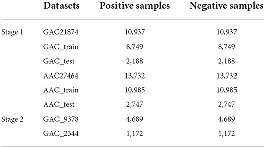
Table 1. Benchmark datasets demonstration.
In addition, the “SupportNum” for each m6A site recorded in RMBase v2.0 was used as the target for regression task. Although the m6A sites recorded in RMBase database can be used to train models for classification, the locations of m6A sites in the database were determined based both on the experimentally measured peak values and the RRACH motif. For each m6A site recorded in the database, the “SupportNum” represents how many experiments have demonstrated that the corresponding adenine can be modified. Intuitively, the more times the m6A site was identified by experiments, the higher confidence we have for the m6A site to be a realistic m6A site. Figure 1 shows the “SupportNum” distribution in our datasets. To take advantage of the information of “SupportNum” and give reasonable confidence for the predicted m6A sites of the classification model, we set a regression task in our multi-task learning architecture with the “SupportNum” as the target. Since the value range of “SupportNum” is relatively large, we first normalized it to [0,1]. Sklearn's Minmax Scaler was used for this normalization process.
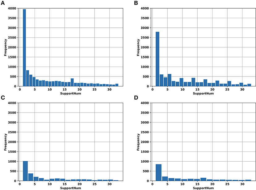
Figure 1. The histogram of “SupportNum” on different datasets. (A) AAC_train; (B) GAC_train; (C) AAC_test; (D) GAC_test.
For the second stage model, we collected base resolution m6A sites of Saccharomyces cerevisiae from m6A-Atlas (www.xjtlu.edu.cn/biologicalsciences/atlas) (Tang et al., 2021) as positive samples. Totally, 10,562 m6A sites were obtained, which are all with the central motif of GAC. Because the second stage model is used to identify base resolution m6A sites from low-resolution m6A sites, we used the low-resolution m6A sites recorded in RMBase 2.0 but not in m6A-Atlas as negative samples in the current study. Note, the negative samples were also with central motif of GAC. Thus, we obtained 10,562 positive samples and 14,810 negative samples. The redundancies of both positive and negative samples were removed by CD-HIT with a cutoff of 0.7. Thus, we got 5,861 positive samples and 8,924 negative samples. To obtain a balanced dataset, 5,861 negative samples were randomly selected to build the final dataset. The dataset was further divided into training and independent test set at a ratio of 4:1 (Table 1).
Model construction
Overall framework of the two-stage model
To fully use the existing experimental data and simulate the calibration process, we proposed a two-stage predictor. The flowchart for building our model is shown in Figure 2. The benchmark datasets collected from RMBase v2.0 were used to train and test our first stage model. A multi-task model was built in the first stage to classify the low resolution m6A sites and other non-m6A sites, which can also give a reasonable confidence for the classification result based on the regression task. For the second stage, we collected the data from m6A-Atlas to build our model which is used to identify the base resolution m6A sites from the low resolution m6A sites. The second-stage model was trained by using a transfer learning strategy based on the first-stage model.

Figure 2. The overall flow chart of MTDeepM6A-2S. (a) The diagram of the two-stage model. The stage I model is used to discriminate low-resolution m6A sites from non-m6A sites and the stage II model is used to identify high-resolution m6A sites from low-resolution m6A sites. Three deep networks were used to build the stage I model which are (b) CNN network, (c) CNN+TRANSFORMER network and (d) CNN+LSTM network.
The framework for the first stage model
The previous methods used to predict RNA m6A sites were mostly single-task learning for classification. However, we used a multi-task architecture to build the first-stage model. As shown in Figure 2a, the input for our model is the sequences of the RNA segments, then the sequences were transformed as numerical matrices by the one-hot encoding with A, U, C, G, N represented as (1,0,0,0), (0,1,0,0), (0,0,1,0), (0,0,0,1) and (0,0,0,0), respectively, where N is a padding pseudo nucleotide when the RNA segment is out of the genome. Then, the 4*601 matrix obtained by one-hot encoding was fed into the shared deep network of the multi-task model, and then the latent features encoded by shared deep networks were fed to the two task-specific networks. In this study, we compared three different shared deep networks which are CNN, CNN+BiLSTM and CNN+TRANSFORMER to select a better shared deep network. The three deep networks were explained as follows.
For the shared CNN network (Figure 2b) of the multi-task model, we used a 1D convolution layer to extract the global information of the sequence. The number of kernels was set to 16 but the size of the kernel used in the 1D CNN was optimized. Next, the output of the 1D CNN was normalized with a layer of Group normalization (GN) (Wu and He, 2018), for which the number of groups was set to 4.
For the shared CNN+BiLSTM network (Figure 2d) of the multi-task model, we added a BiLSTM layer based on the CNN network. The hidden unit of the cell of the BiLSTM was set as 8. BiLSTM overcomes the problem of not being able to retrieve information from upstream and downstream sequences.
For the shared CNN+TRANSFORMER network (Figure 2c) of the multi-task model, we added a position embedding layer and an Encoder of the Transformer (Vaswani et al., 2017) based on the CNN network. The Encoder is composed of a position embedding layer, a multi-head self-attention mechanism and a position-wise fully connected feed-forward network. The head number was set to 2. The “elu” activation function was used in all the three deep networks.
After the three deep networks, we used a 1D pooling layer to reduce the dimension of the features, the size of the kernel of the 1D pooling layer was optimized. After the pooling layer, a fully connected layer with 64 hidden nodes was added. To prevent overfitting, a dropout layer was added after the fully connected layer, and the dropout ratio was also optimized.
In the output layer, there are two outputs. For the classification task, the “softmax” activation function was used, and the categorical cross entropy was used as the loss function. For the regression task, the activation function “elu” was used and the “logcosh” was used as the loss function. Thus, the loss function of the whole multi-task can be expressed as follows:
where, N represents the number of samples in the dataset, and mean the real label and predictive probability of the ith sample for the classification task, respectively. and ŷi show the real label and the predictive values of the ith sample for the regression task, and the former part of the multi-task loss (Lossmulti) is the categorical cross entropy for the classification task, and the latter part is the log-cosh loss for the regression task. According to this loss function, the information of the label of the auxiliary task (regression task) might be able to help improve the predictive accuracy of the classification task.
At last, we used Stochastic Gradient Descent (SGD) as the optimization algorithm. Our deep learning network was built based on Keras version 2.2.4
Transfer learning for building the second stage model
Considering the similarity between the classification tasks of the two stages, we transferred the feature extraction layers of the first-stage model to build our second-stage model. Specifically, during transfer learning, the feature extraction layers (all layers except the output layer) and corresponding weights of the first-stage model were used as the initial parameters for the second-stage model and then all the weights of the second stage model were optimized without freezing in the training process.
To train our model, we needed to determine the network hyperparameters mentioned in Section Model construction such as dropout ratio, pool size and kernel size. We also needed to determine some general hyperparameters such as learning rate, batch size, and epochs. In this study, we used the module GridSearchCV of sklearn package to determine the hyperparameters of the first-stage model by 5-fold cross-validation. Supplementary Table S2 shows the ranges of hyperparameters that were optimized by GridSearchCV. Supplementary Table S3 shows the optimized values for the hyperparameters of the deep network.
Evaluation criteria
To evaluate the performance of the predictors, we calculated four metrics which are sensitivity (Sn), specificity (Sp), accuracy (Acc), and Matthews correlation coefficient (MCC). The four parameters were defined as follows:
where TP, TN, FP, and FN represent the number of true positive, true negative, false positive, and false negative, respectively. Sensitivity and specificity indicate the ratios of correctly predicted positive samples and negative samples, respectively. Accuracy represents the ratio of correctly predicted samples. The Matthews correlation coefficient is a balanced measurement index, which can be used even when the category data is unbalanced.
In addition, we plotted Receiver Operating Characteristic (ROC) curves and Precision-Recall curves (PRC). ROC curve is a comprehensive index to reflect the continuous variables of sensitivity and specificity, thus revealing the relationship between sensitivity and specificity. PRC reflects the balance between the accuracy of positive samples recognition and the coverage ability of the classifier. AUROC (area under ROC curve) and AUPRC (area under PRC curve) are the area under the ROC curve and the area under the precision-recall curve, respectively. The larger the AUROC and AUPRC are, the better the classifier is.
Pearson correlation coefficient is used as the index to evaluate the regression task, which can be calculated as follow:
where, Xi and Yi represent the predicted target value and the actual target value of the sample i, respectively. Pearson correlation coefficient, also known as Pearson product-moment correlation coefficient, is a statistical quantity used to reflect the similarity degree of two variables. Its value range is [−1, 1], and when it equals 0, it indicates no correlation.
Results
Results for the first-stage model
The performance of CNN, CNN+BiLSTM and CNN+TRANSFORMER frameworks under multi-task learning was evaluated by 5-fold cross validation. As shown in Table 2 and Figure 3, for the classification task, the model with CNN+BiLSTM framework achieved the highest Acc, MCC, AUPRC, and AUROC for both GAC_train and AAC_train. The Acc, MCC, AUPRC and AUROC for GAC_train are 0.7919, 0.5869, 0.8592, and 0.8728, respectively, and the Acc, MCC, AUPRC and AUROC for AAC_train are 0.8002, 0.6019, 0.8636, and 0.8787, respectively. For the regression task, the model with CNN+BiLSTM framework also performed best, which achieved the highest Pearson correlation coefficient of 0.6186 and 0.6131 for GAC_train and AAC_train, respectively. The details of the predictive result for each fold based on CNN+BiLSTM framework are shown in Supplementary Tables S4–S6 for the three training datasets, respectively. Thus, the model with CNN+BiLSTM framework was selected as the final model for multi-task learning. We inferred that the CNN+BiLSTM model performs better than other models because we used a long sequence of RNA segment of 601 nucleotides. As shown in Tang et al.'s work (Tang et al., 2018), the bi-deep RNN-based model slightly outperforms CNN and Transformer models on modeling subject-verb agreement over long distances.
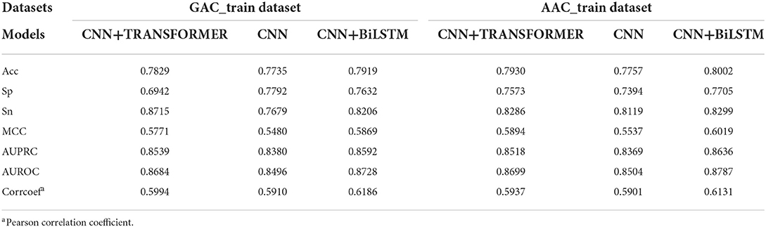
Table 2. Performance of three multi-task deep learning models on the two training datasets.
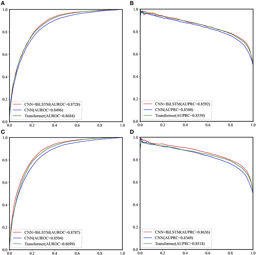
Figure 3. The ROC curves and PRC curves based on the cross-validation results of the three network frameworks on GAC_train and AAC_train. (A) ROC curves for GAC_train; (B) PRC curves for GAC_train; (C) ROC curves for AAC_train; (D) PRC curves for AAC_train.
Table 3 shows the performance of CNN+BiLSTM model on GAC_test under multi-task learning. The model built based on GAC_train performs well on its test dataset with values of 0.7938, 0.6914, 0.8961, 0.6002, 0.8753, and 0.8740 for Acc, Sp, Sn, MCC, AUPRC, and AUROC, respectively. Moreover, the performance of the model established on AAC_train is superior to the model established on GAC_train on GAC_test. However, the difference is small.
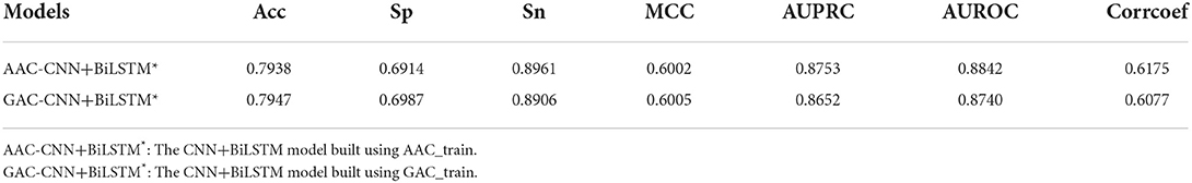
Table 3. Performance of CNN+BiLSTM model on GAC_test under multi-task learning.
Table 4 shows the performance of CNN+BiLSTM model on AAC_test under multi-task learning. The model established with AAC_train also performs well on its test dataset with values of 0.7968, 0.7143, 0.8793, 0.6019, 0.8698, and 0.8792 for Acc, Sp, Sn, MCC, AUPRC, and AUROC, respectively. Again, the model established on AAC_train has achieved better performance on AAC_test than the model established on GAC_train.
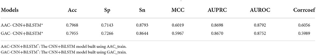
Table 4. Performance of CNN+BiLSTM model on AAC_test under multi-task learning.
Tables 3, 4 indicate the model with CNN+BiLSTM framework trained on AAC_train outperforms the corresponding model trained on GAC_train for the two independent test sets. One of the possible reasons is that AAC_train is bigger than GAC_train. To validate this hypothesis, we built a model based on the combined dataset with both GAC_train and AAC_train. Table 5 shows that the performance of the model established on the combined dataset is superior to the model built on single training dataset according to the Acc, MCC, AUPRC, and AUROC values for classification and Pearson correlation coefficient values for regression. Supplementary Figure S1 shows the corresponding ROC curves and PRC curves.

Table 5. Performance of the CNN+BiLSTM model built on the combined dataset of GAC_train and AAC_train.
For the regression task, we compared the Pearson correlation coefficient obtained by our regression task with that obtained based on the predicted probability of the classification task and the target values of the regression task. Figure 4 shows the Pearson correlation coefficient values under different conditions. It indicates that the Pearson correlation coefficients obtained by our regression task are significantly better than the Pearson correlation coefficients obtained based on the predicted probability of the classification task.
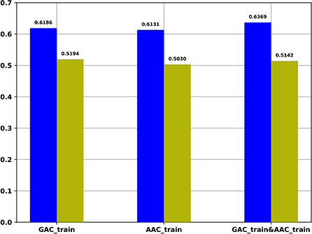
Figure 4. The Pearson correlation coefficient of multi-task models on different training datasets. Blue: The Pearson correlation coefficient obtained by regression task of multi-task models; Yellow: The Pearson correlation coefficient values obtained based on the predicted probability of the classification task of multi-task models and the target values of the regression task of multi-task models.
Results for the second-stage model
Transfer learning was used to build the second-stage model based on the model built in the first stage. In this stage, the hyperparameter “epochs” were optimized to build our model whose range was from 16 to 256. Figure 5 shows the cross validation AUROCs of different epochs, which indicates the highest AUROC (0.7304) is obtained when epochs is 64. To investigate if the performance of transfer learning is superior to that of training from scratch, the same network without using the weights obtained from the first-stage model was trained. We set up two groups of epochs, one is from 16 to 256 and the other one is from 76 to 316 as the epochs used for building the first-stage model is 60. Figure 5 shows that the highest AUROCs obtained for the two groups of parameters are 0.7059 and 0.7030, respectively, which are lower than the AUROC obtained from transfer learning. Thus, our results demonstrate that transfer learning outperforms learning from scratch in this study. The details of the predictive result for each fold based on the final second-stage model are shown in Supplementary Table S7, and the ROC and PRC curves for the cross validation results are shown in Supplementary Figure S2.

Figure 5. Cross-validation performances of three different learning strategies by using different epochs for the second-stage model. TF: Transfer learning; Scratch1: Learning from scratch with epochs from 16 to 256; Scratch2: Learning from scratch with epochs from 76 to 316.
Comparison with existing predictors
Because most of the existing predictors were built based on the dataset which is composed of 1,307 base resolution data with GAC motif in the center, we decided to compare our second-stage model with these methods on the independent test set GAC_2344. Although several models such as BEMRP (Huang et al., 2018), m6Apred (Chen et al., 2015c), iRNA(m6A)-PseDNC (Chen et al., 2018) and iRNA-methyl (Chen et al., 2015b) have been developed to predict m6A sites of Saccharomyces cerevisiae. However, only m6Apred, iRNA(m6A)-PseDNC and iRNA-methyl are available now, Table 6 and Figure 6 show that our model substantially outperforms these three models on all the evaluation metrics except sensitivity. We noted that the model iRNA(m6A)-PseDNC even got a negative MCC. In the work for building the model iRNA(m6A)-PseDNC (Chen et al., 2018), the 1,307 negative samples were specifically selected according to the Euclidean distance (based on the 22 features) to the center of all 33,280 negative samples.
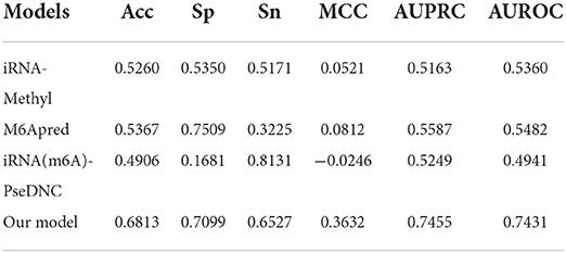
Table 6. Performance of different models on GAC_test.
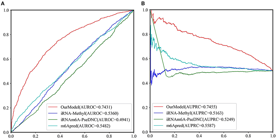
Figure 6. The ROC curves and PRC curves based on the predictive results of the independent test set GAC_2344 by our model and the other three methods. (A) ROC curves; (B) PRC curves.
Discussions
Results of single-task models
In order to evaluate the efficacy of multi-task learning architecture, we conducted the two single-task learnings, i.e., classification task learning and regression task learning, based on the selected CNN+BiLSTM network, respectively. Table 7 shows the cross validation results of the single-task classification models on the two training datasets. According to AUROC, the performance of the multi-task model is a bit better than that of the single-task classification model on AAC_train, however, the performance of the multi-task model is a little worse than that of the single-task classification model on GAC_train. To further demonstrate the effectiveness of multi-task architecture, we also evaluated the performance on the dataset including both AAC_train and GAC_train. As shown in Table 7, the AUROC (0.8871), AUPRC (0.8738), MCC (0.6196) of the multi-task model are all better than that of the single-task classification model on this dataset.
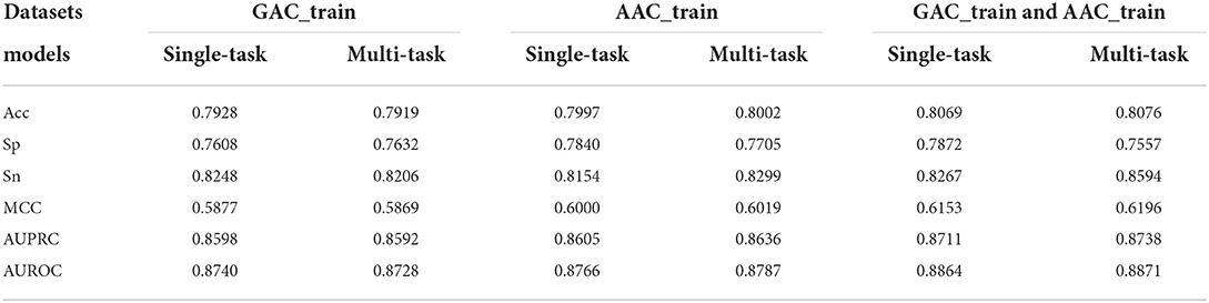
Table 7. Performance comparison between the single-task classification models and the classification task of the multi-task models based on GAC_train, AAC_train, and GAC_train and AAC train, respectively.
Table 8 shows the cross validation results of the single-task regression models on AAC_train, GAC_train and the combined dataset of AAC_train and GAC_train. It shows that the performance of multi-task models is a little bit better than that of the single-task regression models on the three datasets according to the Pearson correlation coefficients.
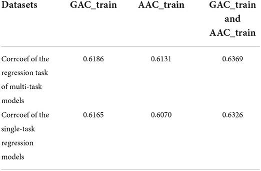
Table 8. The cross-validation Pearson correlation coefficient of single-task regression models and multi-task models on GAC_train, AAC_train and GAC_train and AAC_train, respectively.
By comparing the performance between multi-task learning and single-task learning on the three datasets, GAC_train, AAC_train and the combined dataset. Our results show that the AUROCs of the classification-task are 0.8728 and 0.8740 based on multi-task learning and single-task learning for GAC_train, respectively, and the correlation coefficients of the regression task are 0.6186 and 0.6165 based on multi-task learning and single-task learning, respectively. On AAC_train, the AUROCs of the classification-task are 0.8787 and 0.8766 based on multi-task learning and single-task learning, respectively, and the correlation coefficients of the regression task are 0.6131 and 0.6070 based on multi-task learning and single-task learning, respectively. On the combined dataset with GAC_train and AAC_train, the AUROCs of the classification-task are 0.8871 and 0.8864 based on multi-task learning and single-task learning, respectively, and the correlation coefficients of the regression task are 0.6369 and 0.6326 based on multi-task learning and single-task learning, respectively. Thus, the multi-task learning outperforms the single-task learning for 5 of the 6 tasks on the three datasets. In addition, the multi-task learning framework is more efficient than single-task model because it can complete the two tasks simultaneously. Overall, our results indicate that the multi-task model slightly outperforms the single-task models.
Performance of the first-stage model based on different loss weights and task-specific networks
To evaluate the effectiveness of different loss weights on our first-stage model, we used the strategy developed in Cipolla et al.'s work (Cipolla et al., 2018) to optimize the weights by using uncertainty and obtained a weights ratio of 0.06:1.85. Based on these weights, we validated the model based on AAC dataset and obtained a 5-fold cross validation AUROC of 0.8517, which is less than the value (0.8787) obtained based on the weight ratio of 1.0:1.0.
In addition, we set up two dense layers with 64 nodes as the task-specific networks for the two tasks, respectively, to check if the performance could be improved. Figure 7 shows that the model with task-specific dense network achieves similar results to our original model.
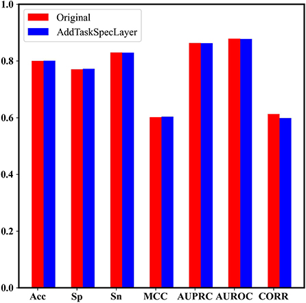
Figure 7. The performance comparison between the model with task-specific dense network and our original model.
Analysis of sequences in the benchmark datasets of the two stages
Table 2 and Figure 5 show the AUROC of the first-stage model is higher than the second stage model, one possible reason is the discrepancy between positive and negative samples in the benchmark datasets of the two stages is different. Supplementary Figure S3 shows the graphical sequence logo generated by Two Sample Logo (Vacic et al., 2006) for the two benchmark datasets, which indicates the discrepancy between positive and negative samples of the training dataset of the first stage (upper panel) is larger than that of the second stage (lower panel). Thus, a two-stage model would be helpful for predicting m6A sites.
Conclusions
In this study, we built a two-stage model, MTDeepM6A-2S, which can serially predict low resolution and base resolution m6A sites of Saccharomyces cerevisiae in the first and second stages. We used both the extensive low resolution data and the less extensive base resolution data to build our model, so as to simulate the process of wet experiments in which the base resolution m6A sites can be identified by post-calibration. To use the “SupportNum” information recorded in RMBase, we adopted a multi-task learning algorithm to build our first-stage model through which we can not only predict m6A sites of Saccharomyces cerevisiae but also give a reasonable confidence for the predictive results. Three deep learning networks were tried in this study, which are based on CNN, CNN+BiLSTM and CNN+TRANSFORMER frameworks. Our results indicate that the model with CNN+BiLSTM framework achieves the best performance. Further analysis also shows that the model based on multi-task learning is superior to the single-task learning. In the light of the similarity between the classification tasks of the two stages, transfer learning was employed to build the second-stage model so that the network weights obtained from the first stage could be used. In addition, the generalization of our model was evaluated on an independent test dataset, which indicates our model is substantially superior to the existing predictor, so that our model could be a useful tool for the community.
Data availability statement
Publicly available datasets were analyzed in this study. This data can be found here: https://github.com/zhu313/MTDeepM6A-2S.
Author contributions
XZ and SB conceived the study. XZ and HW designed the experiments. HW, SZ, and YC performed the experiments, analyzed the data, and wrote the article. All authors have read and agreed to the published version of the manuscript.
Funding
This work was supported in part by National Natural Science Foundation of China (Grant Number: 21403002).
Conflict of interest
The authors declare that the research was conducted in the absence of any commercial or financial relationships that could be construed as a potential conflict of interest.
Publisher's note
All claims expressed in this article are solely those of the authors and do not necessarily represent those of their affiliated organizations, or those of the publisher, the editors and the reviewers. Any product that may be evaluated in this article, or claim that may be made by its manufacturer, is not guaranteed or endorsed by the publisher.
Supplementary material
The Supplementary Material for this article can be found online at: https://www.frontiersin.org/articles/10.3389/fmicb.2022.999506/full#supplementary-material
References
Adams, J. M., and Cory, S. (1975). Modified nucleosides and bizarre 5'-termini in mouse myeloma mRNA. Nature 255, 28–33. doi: 10.1038/255028a0
Aguilo, F., Zhang, F., Sancho, A., Fidalgo, M., Di Cecilia, S., Vashisht, A., et al. (2015). Coordination of m(6)A mRNA methylation and gene transcription by ZFP217 regulates pluripotency and reprogramming. Cell Stem Cell. 17, 689–704. doi: 10.1016/j.stem.2015.09.005
Akbar, S., and Hayat, M. (2018). iMethyl-STTNC: Identification of N(6)-methyladenosine sites by extending the idea of SAAC into Chou's PseAAC to formulate RNA sequences. J. Theor. Biol. 455, 205–211. doi: 10.1016/j.jtbi.2018.07.018
Caruana, R. (1998). “Multitask learning,” in Learning to Learn, eds S. Thrun, and L. Pratt (Boston, MA: Springer), 95–133.
Chen, K., Lu, Z., Wang, X., Fu, Y., Luo, G. Z., Liu, N., et al. (2015a). High-resolution N(6) -methyladenosine (m(6) A) map using photo-crosslinking-assisted m(6) A sequencing. Angew. Chem. Int. Ed. Engl. 54, 1587–1590. doi: 10.1002/anie.201410647
Chen, K., Wei, Z., Zhang, Q., Wu, X., Rong, R., Lu, Z., et al. (2019). WHISTLE: a high-accuracy map of the human N6-methyladenosine (m6A) epitranscriptome predicted using a machine learning approach. Nucleic Acids Res. 47, e41. doi: 10.1093/nar/gkz074
Chen, W., Ding, H., Zhou, X., Lin, H., and Chou, K. C. (2018). iRNA(m6A)-PseDNC: Identifying N-6-methyladenosine sites using pseudo dinucleotide composition. Anal. Biochem. 561–562, 59–65. doi: 10.1016/j.ab.2018.09.002
Chen, W., Feng, P., Ding, H., and Lin, H. (2016). Identifying N (6)-methyladenosine sites in the Arabidopsis thaliana transcriptome. Mol. Genet. Genomics. 291, 2225–2229. doi: 10.1007/s00438-016-1243-7
Chen, W., Feng, P., Ding, H., Lin, H., and Chou, K. C. (2015b). iRNA-methyl: identifying N(6)-methyladenosine sites using pseudo nucleotide composition. Anal. Biochem. 490, 26–33. doi: 10.1016/j.ab.2015.08.021
Chen, W., Tang, H., and Lin, H. (2017). MethyRNA: a web server for identification of N(6)-methyladenosine sites. J. Biomol. Struct. Dyn. 35, 683–687. doi: 10.1080/07391102.2016.1157761
Chen, W., Tran, H., Liang, Z., Lin, H., and Zhang, L. (2015c). Identification and analysis of the N(6)-methyladenosine in the Saccharomyces cerevisiae transcriptome. Sci. Rep. 5, 13859. doi: 10.1038/srep13859
Chen, Z., Zhao, P., Li, F., Wang, Y., Smith, A. I., Webb, G. I., et al. (2020). Comprehensive review and assessment of computational methods for predicting RNA post-transcriptional modification sites from RNA sequences. Brief. Bioinformatics 21, 1676–1696. doi: 10.1093/bib/bbz112
Cipolla, R., Gal, R., and Kendall, A. (2018). “Multi-task learning using uncertainty to weigh losses for scene geometry and semantics,” in Proceedings of the IEEE/CVF Conference on Computer Vision and Pattern Recognition, 7482–7491.
Desrosiers, R., Friderici, K., and Rottman, F. (1974). Identification of methylated nucleosides in messenger RNA from Novikoff hepatoma cells. Proc. Natl. Acad. Sci. U. S. A. 71, 3971–3975. doi: 10.1073/pnas.71.10.3971
Ditzler, G., Polikar, R., and Rosen, G. (2015). Multi-layer and recursive neural networks for metagenomic classification. IEEE Trans. Nanobiosci. 14, 608–616. doi: 10.1109/TNB.2015.2461219
Dominissini, D., Moshitch-Moshkovitz, S., Schwartz, S., Salmon-Divon, M., Ungar, L., Osenberg, S., et al. (2012). Topology of the human and mouse m6A RNA methylomes revealed by m6A-seq. Nature 485, 201–206. doi: 10.1038/nature11112
Fu, L., Niu, B., Zhu, Z., Wu, S., and Li, W. (2012). CD-HIT: accelerated for clustering the next-generation sequencing data. Bioinformatics 28, 3150–3152. doi: 10.1093/bioinformatics/bts565
Furuichi, Y., Morgan, M., Shatkin, A. J., Jelinek, W., Salditt-Georgieff, M., Darnell, J. E., et al. (1975). Methylated, blocked 5 termini in HeLa cell mRNA. Proc. Natl. Acad. Sci. U. S. A. 72, 1904–1908. doi: 10.1073/pnas.72.5.1904
Fustin, J. M., Doi, M., Yamaguchi, Y., Hida, H., Nishimura, S., Yoshida, M., et al. (2013). RNA-methylation-dependent RNA processing controls the speed of the circadian clock. Cell 155, 793–806. doi: 10.1016/j.cell.2013.10.026
Garcia-Campos, M. A., Edelheit, S., Toth, U., Safra, M., Shachar, R., Viukov, S., et al. (2019). Deciphering the “m(6)A code” via antibody-independent quantitative profiling. Cell 178, 731–747.e716. doi: 10.1016/j.cell.2019.06.013
Huang, Y., He, N., Chen, Y., Chen, Z., and Li, L. (2018). BERMP: a cross-species classifier for predicting m(6)A sites by integrating a deep learning algorithm and a random forest approach. Int. J. Biol. Sci. 14, 1669–1677. doi: 10.7150/ijbs.27819
Jia, C. Z., Zhang, J. J., and Gu, W. Z. (2016). RNA-MethylPred: a high-accuracy predictor to identify N6-methyladenosine in RNA. Anal. Biochem. 510, 72–75. doi: 10.1016/j.ab.2016.06.012
Khan, A., Rehman, H. U., Habib, U., and Ijaz, U. (2020). Detecting N6-methyladenosine sites from RNA transcriptomes using random forest. J Comput Sci. Neth. 47, 101238. doi: 10.1016/j.jocs.2020.101238
Li, G. Q., Liu, Z., Shen, H. B., and Yu, D. J. (2016). TargetM6A: identifying N(6)-methyladenosine sites from RNA sequences via position-specific nucleotide propensities and a support vector machine. IEEE Trans. Nanobiosci. 15, 674–682. doi: 10.1109/TNB.2016.2599115
Li, J., He, S., Guo, F., and Zou, Q. (2021). HSM6AP: a high-precision predictor for the Homo sapiens N6-methyladenosine (m∧6 A) based on multiple weights and feature stitching. RNA Biol. 18, 1882–1892. doi: 10.1080/15476286.2021.1875180
Linder, B., Grozhik, A. V., Olarerin-George, A. O., Meydan, C., Mason, C. E., Jaffrey, S. R., et al. (2015). Single-nucleotide-resolution mapping of m6A and m6Am throughout the transcriptome. Nat. Methods 12, 767–772. doi: 10.1038/nmeth.3453
Liu, J., and Jia, G. (2014). Methylation modifications in eukaryotic messenger RNA. J. Genet. Genomics 41, 21–33. doi: 10.1016/j.jgg.2013.10.002
Liu, L., Lei, X., Fang, Z., Tang, Y., Meng, J., Wei, Z., et al. (2020a). LITHOPHONE: improving lncRNA methylation site prediction using an ensemble predictor. Front. Genet.11, 545. doi: 10.3389/fgene.2020.00545
Liu, L., Lei, X., Meng, J., and Wei, Z. (2020b). WITMSG: large-scale prediction of human intronic m(6)A RNA methylation sites from sequence and genomic features. Curr. Genomics 21, 67–76. doi: 10.2174/1389202921666200211104140
Liu, Z., Xiao, X., Yu, D. J., Jia, J., Qiu, W. R., Chou, K. C., et al. (2016). pRNAm-PC: predicting N(6)-methyladenosine sites in RNA sequences via physical-chemical properties. Anal. Biochem. 497, 60–67. doi: 10.1016/j.ab.2015.12.017
Luo, G. Z., MacQueen, A., Zheng, G. Q., Duan, H. C., Dore, L. C., Lu, Z. K., et al. (2014). Unique features of the m(6)A methylome in Arabidopsis thaliana. Nat. Commun. 5, 5630. doi: 10.1038/ncomms6630
Ma, J. Z., Yang, F., Zhou, C. C., Liu, F., Yuan, J. H., Wang, F., et al. (2017). METTL14 suppresses the metastatic potential of hepatocellular carcinoma by modulating N(6) -methyladenosine-dependent primary MicroRNA processing. Hepatology 65, 529–543. doi: 10.1002/hep.28885
Maden, B. E. (1990). The numerous modified nucleotides in eukaryotic ribosomal RNA. Prog. Nucleic Acid Res. Mol. Biol. 39, 241–303. doi: 10.1016/S0079-6603(08)60629-7
Mahmoudi, O., Wahab, A., and Chong, K. T. (2020). iMethyl-deep: N6 methyladenosine identification of yeast genome with automatic feature extraction technique by using deep learning algorithm. Genes 11, 529. doi: 10.3390/genes11050529
Meyer, K. D., Saletore, Y., Zumbo, P., Elemento, O., Mason, C. E., Jaffrey, S. R., et al. (2012). Comprehensive analysis of mRNA methylation reveals enrichment in 3' UTRs and near stop codons. Cell 149, 1635–1646. doi: 10.1016/j.cell.2012.05.003
Nazari, I., Tahir, M., Tayara, H., and Chong, K. T. (2019), iN6.-Methyl (5-step): Identifying RNA N6-methyladenosine sites using deep learning mode via Chou's 5-step rules Chou's general PseKNC. Chemomet. Intelligent Lab. Syst. 193, 103811. doi: 10.1016/j.chemolab.2019.103811
Qiang, X., Chen, H., Ye, X., Su, R., and Wei, L. (2018). M6AMRFS: robust prediction of N6-methyladenosine sites with sequence-based features in multiple species. Front. Genet. 9, 495. doi: 10.3389/fgene.2018.00495
Schwartz, S., Agarwala, S. D., Mumbach, M. R., Jovanovic, M., Mertins, P., Shishkin, A., et al. (2013). High-resolution mapping reveals a conserved, widespread, dynamic mRNA methylation program in yeast meiosis. Cell 155, 1409–1421. doi: 10.1016/j.cell.2013.10.047
Sun, W. J., Li, J. H., Liu, S., Wu, J., Zhou, H., Qu, L. H., et al. (2016). RMBase: a resource for decoding the landscape of RNA modifications from high-throughput sequencing data. Nucleic Acids Res. 44, D259–265. doi: 10.1093/nar/gkv1036
Sun, Z., Zheng, S., Zhao, H., Niu, Z., Lu, Y., Pan, Y., et al. (2021). To improve the predictions of binding residues with DNA, RNA, carbohydrate, and peptide via multi-task deep neural networks. IEEE ACM Trans. Comput. Biol. Bioinform. doi: 10.1109/TCBB.2021.3118916
Tang, G., Müller, M., Rios, A., and Sennrich, R. (2018). “Why self-attention? A targeted evaluation of neural machine translation architectures,” in Proceedings of the 2018 Conference on Empirical Methods in Natural Language Processing, 4263–4272.
Tang, Y., Chen, K., Song, B., Ma, J., Wu, X., and Xu, Q. (2021), m6A.-Atlas: a comprehensive knowledgebase for unraveling the N6-methyladenosine (m6A) epitranscriptome. Nucleic Acids Res. 49, D134–D143. doi: 10.1093/nar/gkaa692 .
Vacic, V., Iakoucheva, L. M., and Radivojac, P. (2006). Two Sample Logo: a graphical representation of the differences between two sets of sequence alignments. Bioinformatics 22, 1536–1537. doi: 10.1093/bioinformatics/btl151
Vandenhende, S., Georgoulis, S., Proesmans, M., Dai, D., and Van Gool, L. (2022). Multi-task Learning for Dense Prediction Tasks: A Survey, IEEE Transactions on Pattern Analysis and Machine Intelligence, 44:3614–3633. doi: 10.1109/TPAMI.2021.3054719
Vaswani, A., Shazeer, N., Parmar, N., Uszkoreit, J., Jones, L., Gomez, A. N., et al. (2017). “Attention is all you need,” in Proceedings of the Proceedings of the 31st International Conference on Neural Information Processing Systems (Curran Associates Inc.).
Vu, L. P., Pickering, B. F., Cheng, Y., Zaccara, S., Nguyen, D., Minuesa, G., et al. (2017). The N(6)-methyladenosine (m(6)A)-forming enzyme METTL3 controls myeloid differentiation of normal hematopoietic and leukemia cells. Nat. Med. 23, 1369–1376. doi: 10.1038/nm.4416
Wang, X., Lu, Z., Gomez, A., Hon, G. C., Yue, Y., Han, D., et al. (2014). N6-methyladenosine-dependent regulation of messenger RNA stability. Nature 505:117–120. doi: 10.1038/nature12730
Wang, X., and Yan, R. (2018). RFAthM6A: a new tool for predicting m(6)A sites in Arabidopsis thaliana. Plant Mol. Biol. 96, 327–337. doi: 10.1007/s11103-018-0698-9
Wei, C. M., Gershowitz, A., and Moss, B. (1975). Methylated nucleotides block 5' terminus of HeLa cell messenger RNA. Cell 4, 379–386. doi: 10.1016/0092-8674(75)90158-0
Wei, L., Chen, H., and Su, R. (2018), M6APred-EL: a sequence-based predictor for identifying N6-methyladenosine sites using ensemble learning. Mol. Ther. Nucleic Acids 12, 635–644. doi: 10.1016/j.omtn.2018.07.004
Wei, L., Su, R., Wang, B., Li, X., Zou, Q., Gao, X., et al. (2019). Integration of deep feature representations and handcrafted features to improve the prediction of N6-methyladenosine sites. Neurocomputing 324, 3–9. doi: 10.1016/j.neucom.2018.04.082
Wu, X., Wei, Z., Chen, K., Zhang, Q., Su, J., Liu, H., et al. (2019). m6Acomet: large-scale functional prediction of individual m(6)A RNA methylation sites from an RNA co-methylation network. BMC Bioinformatics 20, 223. doi: 10.1186/s12859-019-2840-3
Wu, Y., and He, K. (2018). “Group normalization,” in Proceedings of the Computer Vision – ECCV 2018 ECCV 2018 Lecture Notes in Computer Science, eds V. Ferrari, M. Hebert, C. Sminchisescu, and Y. Weiss (Cham: Springer).
Xiang, S., Liu, K., Yan, Z., Zhang, Y., and Sun, Z. (2016a). RNAMethPre: a web server for the prediction and query of mRNA m6A Sites. PLoS ONE 11, e0162707. doi: 10.1371/journal.pone.0162707
Xiang, S., Yan, Z., Liu, K., Zhang, Y., and Sun, Z. (2016b). AthMethPre: a web server for the prediction and query of mRNA m(6)A sites in Arabidopsis thaliana. Mol. Biosyst. 12, 3333–3337. doi: 10.1039/C6MB00536E
Xing, P., Su, R., Guo, F., and Wei, L. (2017). Identifying N(6)-methyladenosine sites using multi-interval nucleotide pair position specificity and support vector machine. Sci. Rep. 7, 46757. doi: 10.1038/srep46757
Xuan, J. J., Sun, W. J., Lin, P. H., Zhou, K. R., Liu, S., Zheng, L. L., et al. (2018). RMBase v2.0: deciphering the map of RNA modifications from epitranscriptome sequencing data. Nucleic Acids Res. 46, D327–D334. doi: 10.1093/nar/gkx934
Zhang, M., Sun, J. W., Liu, Z., Ren, M. W., Shen, H. B., Yu, D. J., et al. (2016). Improving N-6-methyladenosine site prediction with heuristic selection of nucleotide physical-chemical properties. Ana Biochem. 508, 104–113. doi: 10.1016/j.ab.2016.06.001
Zhang, Y., and Hamada, M. (2018). DeepM6ASeq: prediction and characterization of m6A-containing sequences using deep learning. BMC Bioinformatics 19, 524. doi: 10.1186/s12859-018-2516-4
Zhang, Z., Chen, L. Q., Zhao, Y. L., Yang, C. G., Roundtree, I. A., Zhang, Z., et al. (2019). Single-base mapping of m(6)A by an antibody-independent method. Sci Adv. 5, eaax0250. doi: 10.1126/sciadv.aax0250
Zhang, Z., Chen, T., Chen, H. X., Xie, Y. Y., Chen, L. Q., Zhao, Y. L., et al. (2021). Systematic calibration of epitranscriptomic maps using a synthetic modification-free RNA library. Nat. Methods 18, 1213–1222. doi: 10.1038/s41592-021-01280-7
Zhao, Z., Peng, H., Lan, C., Zheng, Y., Fang, L., Li, J., et al. (2018). Imbalance learning for the prediction of N(6)-Methylation sites in mRNAs. BMC Genomics 19, 574. doi: 10.1186/s12864-018-4928-y
Zhou, J., Lu, Q., Gui, L., Xu, R., Long, Y., Wang, H., et al. (2019). MTTFsite: cross-cell type TF binding site prediction by using multi-task learning. Bioinformatics 35, 5067–5077. doi: 10.1093/bioinformatics/btz451
Zhou, Y., Zeng, P., Li, Y. H., Zhang, Z., and Cui, Q. (2016). SRAMP: prediction of mammalian N6-methyladenosine (m6A) sites based on sequence-derived features. Nucleic Acids Res. 44, e91. doi: 10.1093/nar/gkw104
Zhuang, Y. Y., Liu, H. J., Song, X., Ju, Y., and Peng, H. (2019). A linear regression predictor for identifying N(6)-methyladenosine sites using frequent gapped K-mer pattern. Mol. Ther. Nucleic Acids 18, 673–680. doi: 10.1016/j.omtn.2019.10.001
Keywords: N6-methyladenosine site, BiLSTM, post-transcriptional modification, computational methods, multi-task learning
Citation: Wang H, Zhao S, Cheng Y, Bi S and Zhu X (2022) MTDeepM6A-2S: A two-stage multi-task deep learning method for predicting RNA N6-methyladenosine sites of Saccharomyces cerevisiae. Front. Microbiol. 13:999506. doi: 10.3389/fmicb.2022.999506
Received: 21 July 2022; Accepted: 16 September 2022;
Published: 05 October 2022.
Edited by:
Hyun-Seob Song, University of Nebraska-Lincoln, United StatesReviewed by:
Yi Xiong, Shanghai Jiao Tong University, ChinaWei Chen, Chengdu University of Traditional Chinese Medicine, China
Copyright © 2022 Wang, Zhao, Cheng, Bi and Zhu. This is an open-access article distributed under the terms of the Creative Commons Attribution License (CC BY). The use, distribution or reproduction in other forums is permitted, provided the original author(s) and the copyright owner(s) are credited and that the original publication in this journal is cited, in accordance with accepted academic practice. No use, distribution or reproduction is permitted which does not comply with these terms.
*Correspondence: Xiaolei Zhu, xlzhu_mdl@hotmail.com; Shoudong Bi, bishoudong@163.com
†These authors have contributed equally to this work