Generalization of Caputo-Fabrizio Fractional Derivative and Applications to Electrical Circuits

Alshabanat, Amal; Jleli, Mohamed; Kumar, Sunil; Samet, Bessem

doi:10.3389/fphy.2020.00064

ORIGINAL RESEARCH article

Front. Phys., 20 March 2020
Sec. Statistical and Computational Physics
Volume 8 - 2020 | https://doi.org/10.3389/fphy.2020.00064

Generalization of Caputo-Fabrizio Fractional Derivative and Applications to Electrical Circuits

Amal Alshabanat¹

Mohamed Jleli¹

Sunil Kumar²^*

Bessem Samet¹

¹Department of Mathematics, College of Science, King Saud University, Riyadh, Saudi Arabia
²Department of Mathematics, National Institute of Technology, Jamshedpur, India

A new fractional derivative with a non-singular kernel involving exponential and trigonometric functions is proposed in this paper. The suggested fractional operator includes as a special case Caputo-Fabrizio fractional derivative. Theoretical and numerical studies of fractional differential equations involving this new concept are presented. Next, some applications to RC-electrical circuits are provided.

1. Introduction

In the recent decades, the theory of fractional calculus has brought the attention of a great number of researchers in various disciplines. Indeed, it was observed that the use of fractional derivatives is very useful for modeling many problems in engineering sciences (see e.g., [1–10]). Various notions of fractional derivatives exist in the literature. The basic notions are those introduced by Riemann-Liouville and Caputo (see e.g., [11]), which involve the singular kernel $k (t, s) = \frac{{(t - s)}^{- α}}{Γ (1 - α)}$ , 0 < α < 1. These fractional derivatives play an important role for modeling many phenomena in physics. However, as it was mentioned in Caputo and Fabrizio [12], certain phenomena related to material heterogeneities cannot be well-modeled using Riemann-Liouville or Caputo fractional derivatives. Due to this fact, Caputo and Fabrizio [12] suggested a new fractional derivative involving the non-singular kernel $k (t, s) = e^{\frac{- α (t - s)}{1 - α}}$ , 0 < α < 1. Later, Caputo-Fabrizio fractional derivative was used by many authors for modeling various problems in engineering sciences (see e.g., [13–24]). Furthermore, other fractional derivatives with non-singular kernels were introduced by some authors (see e.g., [10, 25–29]).

In this paper, a new fractional derivative with a non-singular kernel involving exponential and trigonometric functions is proposed. The introduced fractional derivative includes as a special case Caputo-Fabrizio fractional derivative. Theoretical and numerical investigations of fractional differential equations involving this new fractional operator are presented. Next, some applications to electrical circuits are provided.

In section 2, some preliminaries on harmonic analysis are presented. In section 3, we develop a general theory of fractional calculus using an arbitrary non-singular kernel. In section 4, we introduce a generalized Caputo-Fabrizio fractional derivative and study its properties. Some applications to fractional differential equations are given in section 5. A numerical method based on Picard iterations is presented in section 6 with some numerical examples. In section 7, some applications to RC-electrical circuits are provided.

2. Some Preliminaries on Harmonic Analysis

We recall briefly some results on harmonic analysis that will be used later.

Lemma 2.1. Folland [30]. Let ψ ∈ L¹(ℝ) be such that

\int_{ℝ} ψ (t) d t = 1 .

Consider the sequence of functions {_{ψ_ε}ε>0} defined by

ψ_{ε} (t) = \frac{1}{ε} ψ (\frac{t}{ε}), t \in ℝ .

If μ ∈ L¹(ℝ), then

ψ_{ε} * μ \in L^{1} (ℝ), ε > 0

and

lim_{ε \to 0^{+}} ∥ ψ_{ε} * μ - μ ∥_{L^{1} (ℝ)} = 0,

where * denotes the convolution product.

Lemma 2.2. Let ψ ∈ L¹(0, ∞) be such that

\begin{array}{l} \int_{0}^{\infty} ψ (t) d t = 1 . & (2.1) \end{array}

Consider the sequence of functions {_{ψ_ε}ε>0} defined by

ψ_{ε} (t) = \frac{1}{ε} ψ (\frac{t}{ε}), t > 0 .

If μ ∈ L¹(0, ∞), then the sequence of functions ${I_{ε}^{μ}}_{ε > 0}$ defined by

I_{ε}^{μ} (t) = \int_{0}^{t} ψ_{ε} (t - s) μ (s) d s, t > 0

satisfies the following properties:

I_{ε}^{μ} \in L^{1} (0, \infty), ε > 0

and

lim_{ε \to 0^{+}} ∥ I_{ε}^{μ} - μ ∥_{L^{1} (0, \infty)} = 0 .

Proof: For any function f defined almost every where in (0, ∞), let

\begin{array}{l} \tilde{f} (t) = {\begin{matrix} f (t) & a.e. & t > 0, \\ 0 & if & t \leq 0 . \end{matrix} \end{array}

From (2.1), one has $\tilde{ψ} \in L^{1} (ℝ)$ and

\int_{ℝ} \tilde{ψ} (t) d t = 1 .

Hence, by Lemma 2.1, for all f ∈ L¹(ℝ), we have

\tilde{ψ_{ε}} * f \in L^{1} (ℝ), ε > 0

and

lim_{ε \to 0^{+}} ∥ \tilde{ψ_{ε}} * f - f ∥_{L^{1} (ℝ)} = 0,

where

\tilde{ψ_{ε}} (t) = \frac{1}{ε} \tilde{ψ} (\frac{t}{ε}), t \in ℝ .

In particular, for μ ∈ L¹(0, ∞), we have

\begin{array}{l} \tilde{ψ_{ε}} * \tilde{μ} \in L^{1} (ℝ), ε > 0 & (2.2) \end{array}

and

\begin{array}{l} lim_{ε \to 0^{+}} ∥ \tilde{ψ_{ε}} * \tilde{μ} - \tilde{μ} ∥_{L^{1} (ℝ)} = 0 . & (2.3) \end{array}

For all t > 0, we have

\begin{array}{l} \tilde{ψ_{ε}} * \tilde{μ} (t) = \int_{ℝ} \tilde{ψ_{ε}} (t - s) \tilde{μ} (s) d s \\ = \int_{0}^{t} ψ_{ε} (t - s) μ (s) d s \\ = I_{ε}^{μ} (t) . \end{array}

Hence, using (2.2) and (2.3), one obtains

\int_{0}^{\infty} | I_{ε}^{μ} (t) | d t = \int_{0}^{\infty} | \tilde{ψ_{ε}} * \tilde{μ} (t) | d t \leq ∥ \tilde{ψ_{ε}} * \tilde{μ} ∥_{L^{1} (ℝ)} < \infty

and

\begin{array}{l} ∥ I_{ε}^{μ} - μ ∥_{L^{1} (0, \infty)} = \int_{0}^{\infty} | \tilde{ψ_{ε}} * \tilde{μ} (t) - \tilde{μ} (t) | d t \\ \leq ∥ \tilde{ψ_{ε}} * \tilde{μ} - \tilde{μ} ∥_{L^{1} (ℝ)} \to 0 as ε \to 0^{+} . \end{array}

This completes the proof of Lemma 2.2.

□

Definition 2.1. We say that f is of exponential order θ, if for t large enough, one has

| f (t) | \leq C e^{θ t},

where C > 0 and θ are constants.

We denote by $L {f (t)}$ the Laplace transform of the function f, i.e.,

L {f (t)} (s) = \int_{0}^{\infty} e^{- s t} f (t) d t .

Recall that, if f ∈ C[0, ∞) and f is of exponential order θ, then $L {f (t)} (s)$ exists for s > θ.

We denote by ℕ the set of positive integers.

Lemma 2.3. Schiff [31]. Let n ∈ ℕ. If f ∈ Cⁿ[0, ∞) and for all i = 0, 1, ⋯ , n − 1, the function f⁽ⁱ⁾ is of exponential order, then

\begin{array}{l} L {f^{(n)} (t)} (s) = s^{n} L {f (t)} (s) - \sum_{i = 1}^{n} s^{i - 1} f^{(n - i)} (0) . \end{array}

3. Fractional Derivative With an Arbitrary Non-singular Kernel

We consider the set of non-singular kernel functions

\begin{array}{l} K = {k \in C [0, \infty) \cap L^{1} (0, \infty) : \int_{0}^{\infty} k (σ) d σ = 1} . & (3.1) \end{array}

Definition 3.1. Given $k \in K$ , 0 < α < 1 and f ∈ C¹[0, ∞), the fractional derivative of order α of f with respect to the non-singular kernel function k is defined by

\begin{array}{l} (D_{0, k}^{α} f) (t) = \frac{1}{1 - α} \int_{0}^{t} k (\frac{α (t - s)}{1 - α}) f^{'} (s) d s, t > 0 . \end{array}

Remark 3.1. We can also define $D_{0, k}^{α} f$ for functions f ∈ AC[0, ∞) (f is an absolutely continuous function in [0, ∞)). In this case, f′(t) exists for almost every where t > 0 and f′ ∈ L¹(0, ∞).

The following properties hold.

Theorem 3.1. Let $k \in K$ and f ∈ C¹[0, ∞). Then

(i) For all 0 < α < 1,

lim_{t \to 0^{+}} (D_{0, k}^{α} f) (t) = 0 .

(ii) If f′ ∈ L¹(0, ∞), one has

D_{0, k}^{α} f \in L^{1} (0, \infty), 0 < α < 1

and

lim_{α \to 1^{-}} ∥ D_{0, k}^{α} f - f^{'} ∥_{L^{1} (0, \infty)} = 0 .

Proof: (i) Let 0 < α < 1. For 0 < t<T < ∞, one has

| (D_{0, k}^{α} f) (t) | \leq \frac{{∥ k ∥}_{L^{\infty} (0, T_{α})} ∥ f^{'} ∥_{L^{\infty} (0, T)}}{1 - α} t,

where $T_{α} = \frac{α}{1 - α} T$ . Passing to the limit as t → 0⁺ in the above inequality, (i) follows.(ii) Suppose that f′ ∈ L¹(0, ∞). For 0 < α < 1, let $ε = \frac{1 - α}{α}$ . One has

\begin{array}{l} (D_{0, k}^{α} f) (t) = \frac{ε + 1}{ε} \int_{0}^{t} k (\frac{1}{ε} (t - s)) f^{'} (s) d s \\ = (ε + 1) \int_{0}^{t} \frac{1}{ε} k (\frac{1}{ε} (t - s)) f^{'} (s) d s \\ = (ε + 1) \int_{0}^{t} k_{ε} (t - s) f^{'} (s) d s, t > 0, \end{array}

where

k_{ε} (x) = \frac{1}{ε} k (\frac{x}{ε}), x > 0 .

Hence, using Lemma 2.2, (ii) follows.

□

Definition 3.2. Given $k \in K$ , 0 < α < 1, n ∈ ℕ∪{0} and f ∈ C^{n + 1}[0, ∞), the fractional derivative of order α+n of f with respect to the non-singular kernel k is defined by

(D_{0, k}^{α + n} f) (t) = \frac{1}{1 - α} \int_{0}^{t} k (\frac{α (t - s)}{1 - α}) f^{(n + 1)} (s) d s, t > 0 .

Remark 3.2. We can also define $D_{0, k}^{α + n} f$ for functions f ∈ AC^{n + 1}[0, ∞). In this case, f^{n + 1}(t) exists for almost every where t > 0 and f^{(n + 1)} ∈ L¹(0, ∞).

Similarly to the case n = 0, one has

Theorem 3.2. Let $k \in K$ , n ∈ ℕ ∪{0} and f ∈ C^{n + 1}[0, ∞). Then

(i) For all 0 < α < 1,

lim_{t \to 0^{+}} (D_{0, k}^{α + n} f) (t) = 0 .

(ii) If f^{(n + 1)} ∈ L¹(0, ∞), then

D_{0, k}^{α + n} f \in L^{1} (0, \infty), 0 < α < 1

and

lim_{α \to 1^{-}} ∥ D_{0, k}^{α + n} f - f^{(n + 1)} ∥_{L^{1} (0, \infty)} = 0 .

Remark 3.3. From the assertion (ii) of Theorem 3.2, if f⁽ⁿ⁺¹⁾ ∈ L¹(0, ∞), one has

lim_{α \to 1^{-}} (D_{0, k}^{α + n} f) (t) = f^{(n + 1)} (t), a . e . t > 0 .

Theorem 3.3. Given $k \in K$ , 0 < α < 1, n ∈ ℕ ∪{0} and f ∈ C^{n + 1}[0, ∞) with f⁽ⁱ⁾, i = 0, 1, ⋯ , n, are of exponential order, one has

\begin{array}{l} L {(D_{0, k}^{α + n} f) (t)} (s) \\ = \frac{1}{1 - α} (s^{n + 1} L {f (t)} (s) - \sum_{i = 1}^{n + 1} s^{i - 1} f^{(n + 1 - i)} (0)) L {k_{α} (t)} (s), \end{array}

where

k_{α} (t) = k (\frac{α t}{1 - α}), t > 0 .

Proof: One has

\begin{array}{l} L {(D_{0, k}^{α + n} f) (t)} (s) \\ = \int_{0}^{\infty} e^{- t s} (D_{0, k}^{α + n} f) (t) d t \\ = \int_{0}^{\infty} e^{- t s} (\frac{1}{1 - α} \int_{0}^{t} k (\frac{α (t - σ)}{1 - α}) f^{(n + 1)} (σ) d σ) d t . \end{array}

Using Fubini's theorem, one obtains

\begin{array}{l} L {(D_{0, k}^{α + n} f) (t)} (s) \\ = \frac{1}{1 - α} \int_{0}^{\infty} f^{(n + 1)} (σ) (\int_{σ}^{\infty} e^{- t s} k (\frac{α (t - σ)}{1 - α}) d t) d σ . & (3.2) \end{array}

Using the change of variable τ = t − σ, it holds

\begin{array}{l} \int_{σ}^{\infty} e^{- t s} k (\frac{α (t - σ)}{1 - α}) d t \\ = e^{- σ s} \int_{0}^{\infty} e^{- τ s} k (\frac{α τ}{1 - α}) d τ \\ = e^{- σ s} L {k_{α} (t)} (s) . \end{array}

Hence, by (3.2), one deduces that

L {(D_{0, k}^{α + n} f) (t)} (s) = \frac{1}{1 - α} L {f^{(n + 1)} (t)} (s) L {k_{α} (t)} (s) .

Next, using Lemma 2.3, we obtain

\begin{array}{l} L {(D_{0, k}^{α + n} f) (t)} (s) \\ = \frac{1}{1 - α} (s^{n + 1} L {f (t)} (s) - \sum_{i = 1}^{n + 1} s^{i - 1} f^{(n + 1 - i)} (0)) L {k_{α} (t)} (s), \end{array}

which yields the desired result.

□

4. A Generalized Caputo-Fabrizio Fractional Derivative

Consider the kernel function

k_{a, b} (t) = (\frac{a^{2} + b^{2}}{a}) e^{- a t} cos (b t), t \geq 0,

where a > 0 and b ≥ 0 are constants. It can be easily seen that

\begin{array}{l} k_{a, b} \in K, & (4.1) \end{array}

where $K$ is the set of kernel functions defined by (3.1). Hence, using Definition 3.2, we define the fractional derivative with respect to the kernel function k_{a, b} as follows.

Definition 4.1. Given a > 0, b ≥ 0, 0 < α < 1, n ∈ ℕ∪{0} and f ∈ C^{n + 1}[0, ∞), the fractional derivative of order α+n of f with respect to the kernel function k_{a, b} is defined by

\begin{array}{l} (D_{0, a, b}^{α + n} f) (t) = (\frac{1}{1 - α}) (\frac{a^{2} + b^{2}}{a}) \\ \int_{0}^{t} e^{- \frac{a α (t - s)}{1 - α}} cos (\frac{b α (t - s)}{1 - α}) f^{(n + 1)} (s) d s, t > 0 . \end{array}

Remark 4.1. Taking a = 1 and b = 0 in the above definition, one obtains

(D_{0, 1, 0}^{α + n} f) (t) = (^{C F} D_{0}^{α + n} f) (t), t > 0,

where $^{C F} D_{0}^{α + n}$ is the Caputo–Fabrizio fractional derivative operator of order α + n (see [12]).

Remark 4.2. Definition 4.1 can be extended to the case of functions f ∈ C^{n + 1}[0, T], where 0 < T < ∞.

From (4.1) and Theorem 3.2, one deduces that

Corollary 4.1. Let a > 0, b ≥ 0, n ∈ ℕ∪{0} and f ∈ C^{n + 1}[0, ∞). Then

(i) For all 0 < α < 1,

lim_{t \to 0^{+}} (D_{0, a, b}^{α + n} f) (t) = 0 .

(ii) If f^{(n + 1)} ∈ L¹(0, ∞), then

D_{0, a, b}^{α + n} f \in L^{1} (0, \infty), 0 < α < 1

and

lim_{α \to 1^{-}} ∥ D_{0, a, b}^{α + n} f - f^{(n + 1)} ∥_{L^{1} (0, \infty)} = 0 .

Let

k_{a, b, α} (t) = k_{a, b} (\frac{α t}{1 - α}), t > 0,

that is,

\begin{array}{l} k_{a, b, α} (t) = (\frac{a^{2} + b^{2}}{a}) e^{- \frac{a α t}{1 - α}} cos (\frac{b α t}{1 - α}), t > 0 . \end{array}

Lemma 4.1. Abramowitz and Stegun [32]. Let a > 0, b ≥ 0 and 0 < α < 1. Then

\begin{array}{c} L {k_{a, b, α} (t)} (s) = \frac{(1 - α) (a^{2} + b^{2})}{a} [\frac{(1 - α) s + α a}{{((1 - α) s + α a)}^{2} + b^{2} α^{2}}], \\ s > 0 . \end{array}

Using Theorem 3.3 and Lemma 4.1, one deduces that

Corollary 4.2. Let a > 0, b ≥ 0, 0 < α < 1, n ∈ ℕ∪{0} and f ∈ C^{n + 1}[0, ∞) with f⁽ⁱ⁾, i = 0, 1, ⋯ , n, are of exponential order. Then

\begin{array}{l} L {(D_{0, a, b}^{α + n} f) (t)} (s) \\ = \frac{(a^{2} + b^{2})}{a} (s^{n + 1} L {f (t)} (s) - \sum_{i = 1}^{n + 1} s^{i - 1} f^{(n + 1 - i)} (0)) \\ [\frac{(1 - α) s + α a}{{((1 - α) s + α a)}^{2} + b^{2} α^{2}}], s > 0 . \end{array}

For n = 0, one obtains

Corollary 4.3. Let a > 0, b ≥ 0, 0 < α < 1 and f ∈ C¹[0, ∞) with f is of exponential order. Then

\begin{array}{l} L {(D_{0, a, b}^{α} f) (t)} (s) = \frac{(a^{2} + b^{2})}{a} (s L {f (t)} (s) - f (0)) \\ [\frac{(1 - α) s + α a}{{((1 - α) s + α a)}^{2} + b^{2} α^{2}}] . \end{array}

5. Applications to Fractional Differential Equations

Let a > 0, b ≥ 0, 0 < T < ∞ and 0 < α < 1.

Definition 5.1. Let g ∈ C[0, T]. The fractional integral of order α of g is defined by

\begin{array}{l} (I_{0, a, b}^{α} g) (t) = \frac{a (1 - α)}{a^{2} + b^{2}} g (t) \\ + α (\int_{0}^{t} g (σ) d σ - \frac{b^{2}}{a^{2} + b^{2}} \int_{0}^{t} e^{\frac{- a α (t - σ)}{1 - α}} g (σ) d σ), \\ 0 \leq t \leq T, \end{array}

with $(I_{0, a, b}^{α} g) (0) = 0$ .

Given f₀ ∈ ℝ and g ∈ C¹[0, T] with g(0) = 0, we consider the initial value problem

\begin{array}{l} {\begin{matrix} (D_{0, a, b}^{α} f) (t) = g (t), 0 < t < T, \\ f (0) = f_{0} . \end{matrix} & (5.1) \end{array}

Theorem 5.1. Problem (5.1) admits a unique solution f ∈ C¹[0, T], which is given by

\begin{array}{l} f (t) = f_{0} + (I_{0, a, b}^{α} g) (t), 0 \leq t \leq T . & (5.2) \end{array}

Proof: Let f ∈ C¹[0, T] be a solution of (5.1). One has

\begin{array}{l} {(D_{0, a, b}^{α} f)}^{'} (t) = g^{'} (t), 0 < t < T . & (5.3) \end{array}

By Definition 4.1, one has

\begin{array}{l} {(D_{0, a, b}^{α} f)}^{'} (t) = (\frac{1}{1 - α}) (\frac{a^{2} + b^{2}}{a}) \\ {f^{'} (t) + \int_{0}^{t} \frac{d}{d t} (e^{- \frac{a α (t - s)}{1 - α}} cos (\frac{b α (t - s)}{1 - α})) f^{'} (s) d s} \\ = (\frac{1}{1 - α}) (\frac{a^{2} + b^{2}}{a}) f^{'} (t) \\ - (\frac{a α}{1 - α}) (\frac{1}{1 - α}) (\frac{a^{2} + b^{2}}{a}) \\ \int_{0}^{t} e^{- \frac{a α (t - s)}{1 - α}} cos (\frac{b α (t - s)}{1 - α}) f^{'} (s) d s \\ - (\frac{b α}{1 - α}) (\frac{1}{1 - α}) (\frac{a^{2} + b^{2}}{a}) \\ \int_{0}^{t} e^{- \frac{a α (t - s)}{1 - α}} sin (\frac{b α (t - s)}{1 - α}) f^{'} (s) d s \\ = (\frac{1}{1 - α}) (\frac{a^{2} + b^{2}}{a}) f^{'} (t) - (\frac{a α}{1 - α}) g (t) \\ - (\frac{b α}{1 - α}) (\frac{1}{1 - α}) (\frac{a^{2} + b^{2}}{a}) γ (t), & (5.4) \end{array}

where

γ (t) = \int_{0}^{t} e^{- \frac{a α (t - s)}{1 - α}} sin (\frac{b α (t - s)}{1 - α}) f^{'} (s) d s .

On the other hand,

\begin{array}{l} γ^{'} (t) = \int_{0}^{t} \frac{d}{d t} (e^{- \frac{a α (t - s)}{1 - α}} sin (\frac{b α (t - s)}{1 - α})) f^{'} (s) d s \\ = - (\frac{a α}{1 - α}) γ (t) + (\frac{b α}{1 - α}) \\ \int_{0}^{t} e^{- \frac{a α (t - s)}{1 - α}} cos (\frac{b α (t - s)}{1 - α}) f^{'} (s) d s \\ = - (\frac{a α}{1 - α}) γ (t) + (\frac{a b α}{a^{2} + b^{2}}) g (t) . \end{array}

Integrating the above equality and using that γ(0) = 0, one obtains

γ (t) = \frac{a b α}{a^{2} + b^{2}} \int_{0}^{t} e^{- \frac{a α (t - s)}{1 - α}} g (s) d s .

Hence by (5.4), one deduces that

\begin{array}{l} {(D_{0, a, b}^{α} f)}^{'} (t) = (\frac{1}{1 - α}) (\frac{a^{2} + b^{2}}{a}) f^{'} (t) - (\frac{a α}{1 - α}) g (t) \\ - {(\frac{b α}{1 - α})}^{2} \int_{0}^{t} e^{- \frac{a α (t - s)}{1 - α}} g (s) d s . \end{array}

Next, using (5.3), one obtains

\begin{array}{l} f^{'} (t) = \frac{a^{2} α}{a^{2} + b^{2}} g (t) + (\frac{a b^{2} α^{2}}{(1 - α) (a^{2} + b^{2})}) \int_{0}^{t} e^{- \frac{a α (t - s)}{1 - α}} g (s) d s \\ + \frac{a (1 - α)}{a^{2} + b^{2}} g^{'} (t) . \end{array}

Integrating the above equality, using that f(0) = f₀ and g(0) = 0, it holds

\begin{array}{l} f (t) - f_{0} = (\frac{a^{2} α}{a^{2} + b^{2}}) \int_{0}^{t} g (σ) d σ + \frac{a (1 - α)}{a^{2} + b^{2}} g (t) \\ + (\frac{a b^{2} α^{2}}{(1 - α) (a^{2} + b^{2})}) \int_{0}^{t} \int_{0}^{σ} e^{- \frac{a α (σ - s)}{1 - α}} g (s) d s d σ & (5.5) \end{array}

On the other hand, using Fubini's theorem, one gets

\begin{array}{l} \int_{0}^{t} \int_{0}^{σ} e^{- \frac{a α (σ - s)}{1 - α}} g (s) d s d σ \\ = \int_{0}^{t} g (s) e^{\frac{a α s}{1 - α}} (\int_{s}^{t} e^{- \frac{a α σ}{1 - α}} d σ) d s \\ = (\frac{1 - α}{a α}) \int_{0}^{t} g (s) d s - (\frac{1 - α}{a α}) \int_{0}^{t} e^{- \frac{a α (t - s)}{1 - α}} g (s) d s . & (5.6) \end{array}

It follows from (5.5) and (5.6) that

f (t) = f_{0} + (I_{0, a, b}^{α} g) (t),

i.e., f is a solution of (5.2).

Suppose now that f satisfies (5.2). Clearly, one has f ∈ C¹[0, T]. Since g(0) = 0, one has f(0) = f₀. On the other hand, an elementary calculation shows that $(D_{0, a, b}^{α} f) (t) = g (t)$ for all 0 < t < T. Therefore, f is a solution of (5.2).

□

Consider now the non-linear initial value problem

\begin{array}{l} {\begin{matrix} (D_{0, a, b}^{α} u) (t) = F (t, u (t)), 0 < t < T, \\ u (0) = u_{0}, \end{matrix} & (5.7) \end{array}

where the function F:[0, T] × ℝ → ℝ is continuous and satisfies F(0, u₀) = 0.

Definition 5.2. We say that u ∈ C[0, T] is a weak solution of (5.7), if u solves the integral equation

u (t) = u_{0} + (I_{0, a, b}^{α} F (\cdot, u (\cdot)) (t), 0 \leq t \leq T,

i.e.,

\begin{array}{l} u (t) = u_{0} + \frac{a (1 - α)}{a^{2} + b^{2}} F (t, u (t)) \\ + α (\int_{0}^{t} F (σ, u (σ)) d σ - \frac{b^{2}}{a^{2} + b^{2}} \int_{0}^{t} e^{\frac{- a α (t - σ)}{1 - α}} F (σ, u (σ)) d σ), \end{array}

for all 0 ≤ t ≤ T.

Remark 5.1. Observe that, if F ∈ C¹([0, T] × ℝ), and u ∈ C¹[0, T] is a solution of (5.7), then u ∈ C[0, T] is a weak solution of (5.7).

Theorem 5.2. Suppose that

\begin{array}{l} | F (t, η) - F (t, ξ) | \leq ℓ | η - ξ |, (η, ξ) \in ℝ^{2}, & (5.8) \end{array}

where ℓ > 0 is a constant. If

\begin{array}{l} ℓ (A_{α} + (α + B_{α}) T) < 1, & (5.9) \end{array}

where $A_{α} = \frac{a (1 - α)}{a^{2} + b^{2}}$ and $B_{α} = \frac{α b^{2}}{a^{2} + b^{2}}$ , then (5.7) admits a unique weak solution u^* ∈ C[0, T]. Moreover, for any z₀ ∈ C[0, T], the Picard sequence {z_n} defined by

\begin{array}{l} z_{n + 1} (t) = u_{0} + \frac{a (1 - α)}{a^{2} + b^{2}} F (t, z_{n} (t)) \\ + α (\int_{0}^{t} F (σ, z_{n} (σ)) d σ - \frac{b^{2}}{a^{2} + b^{2}} \int_{0}^{t} e^{\frac{- a α (t - σ)}{1 - α}} F (σ, z_{n} (σ)) d σ), \end{array}

for all 0 ≤ t ≤ T, converges uniformly to u^*.

Proof: Consider the self-mapping H : C[0, T] → C[0, T] defined by

\begin{array}{l} (H u) (t) = u_{0} + \frac{a (1 - α)}{a^{2} + b^{2}} F (t, u (t)) \\ + α (\int_{0}^{t} F (σ, u (σ)) d σ - \frac{b^{2}}{a^{2} + b^{2}} \int_{0}^{t} e^{\frac{- a α (t - σ)}{1 - α}} F (σ, u (σ)) d σ), \end{array}

for all 0 ≤ t ≤ T. We endow C[0, T] with the norm

∥ u ∥_{\infty} = max {| u (t) | : 0 \leq t \leq T} .

Then (C[0, T], ||·||_∞) is a Banach space. For all u, v ∈ C[0, T] and 0 ≤ t ≤ T, using (5.8), one has

\begin{array}{l} | (H u) (t) - (H v) (t) | \\ \leq A_{α} | F (t, u (t)) - F (t, v (t) | + α \int_{0}^{t} | F (σ, u (σ)) - F (σ, v (σ)) | d σ \\ + B_{α} \int_{0}^{t} e^{\frac{- a α (t - σ)}{1 - α}} | F (σ, u (σ)) - F (σ, v (σ)) | d σ \\ \leq ℓ A_{α} ‖ u - v ‖_{\infty} + α ℓ T ‖ u - v ‖_{\infty} + B_{α} ℓ T ‖ u - v ‖_{\infty} \\ = ℓ (A_{α} + (α + B_{α}) T) ‖ u - v ‖_{\infty}, \end{array}

which yields

∥ H u - H v ∥_{\infty} \leq ℓ (A_{α} + (α + B_{α}) T) ∥ u - v ∥_{\infty} .

Hence by (5.9), one deduces that H is a contraction. Therefore, the result follows from Banach fixed point theorem.

□

6. Numerical Solution via Picard Iteration

Consider the initial value problem

\begin{array}{l} {\begin{matrix} (D_{0, 1, 1}^{α} u) (t) = \frac{u (t)}{3} + e^{t}, 0 < t < 1, \\ u (0) = - 3, \end{matrix} & (6.1) \end{array}

where 0 < α < 1. For α = 1, (6.1) reduces to

\begin{array}{l} {\begin{matrix} u^{'} (t) = \frac{u (t)}{3} + e^{t}, 0 < t < 1, \\ u (0) = - 3 . \end{matrix} & (6.2) \end{array}

The exact solution of (6.2) is given by

u_{1} (t) = \frac{3}{2} e^{t} - \frac{9}{2} e^{\frac{t}{3}}, 0 \leq t \leq 1 .

(6.1) is a special case of (5.7) with T = 1, a = b = 1, u₀ = −3 and $F (t, x) = \frac{x}{3} + e^{t}$ . One can check easily that F satisfies (5.8) with $ℓ = \frac{1}{3}$ . Moreover, one has

ℓ (A_{α} + (α + B_{α}) T) = \frac{1}{3} (\frac{1}{2} + α) < 1 .

Hence by Theorem 5.2, (6.1) has a unique weak solution u^* ∈ C[0, 1]. Consider now the Picard sequence {z_n} ⊂ C[0, 1] given by z₀(t) = −3 and

\begin{array}{l} z_{n + 1} (t) = - 3 + \frac{(1 - α)}{2} F (t, z_{n} (t)) \\ + α (\int_{0}^{t} F (σ, z_{n} (σ)) d σ - \frac{1}{2} \int_{0}^{t} e^{\frac{- α (t - σ)}{1 - α}} F (σ, z_{n} (σ)) d σ), & (6.3) \end{array}

for all n = 0, 1, , 2, ⋯ By Theorem 5.2, the sequence {z_n} converges uniformly to u^*. In Figure 1A, for α = 0.95, we plot u₁(t) [the exact solution of (6.2)], z₁(t), z₃(t), and z₁₀(t). In Figure 1B, for α = 0.7, we plot z₁(t), z₃(t), and z₁₀(t).

FIGURE 1

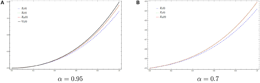
Figure 1. Picard iterations for different values of α. (A) α = 0.95. (B) α = 0.7.

7. Applications to RC Electrical Circuits

In this section, we give some applications to RC electrical circuits using the generalized Caputo-Fabrizio fractional derivative introduced in section 4.

The governing ODE of an RC electrical circuit (see Figure 2) is given by

\begin{array}{l} \frac{d V (t)}{d t} + \frac{V (t)}{R C} = \frac{μ (t)}{R C}, & (7.1) \end{array}

where V is the voltage, R is the resistance, C is the capacitance and μ(t) is the source of volt. In this part, we consider a fractional version of (7.1) using the generalized Caputo-Fabrizio fractional derivative introduced in section 4. Namely, using the following transformation suggested in [33]:

\begin{array}{l} \frac{d}{d t} \to \frac{1}{σ^{1 - α}} D_{0, a, b}^{α}, a > 0, b \geq 0, 0 < α < 1, & (7.2) \end{array}

where σ is a positive parameter having dimensions of seconds, we obtain the fractional differential equation

\begin{array}{l} (D_{0, a, b}^{α} V) (t) + \frac{1}{κ_{α}} V (t) = \frac{1}{κ_{α}} μ (t), & (7.3) \end{array}

where

κ_{α} = \frac{R C}{σ^{1 - α}} .

FIGURE 2

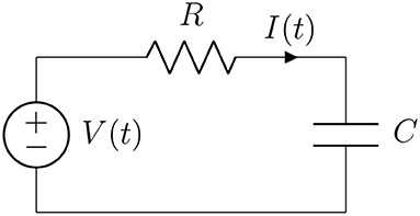
Figure 2. RC circuit.

We consider (7.3) with the source term

μ (t) = sin (ϕ t)

and the initial condition

\begin{array}{l} V (0) = 0 . & (7.4) \end{array}

In this case, (7.3) reduces to

(D_{0, a, b}^{α} V) (t) = A V (t) + B sin (ϕ t),

where $A = - \frac{1}{κ_{α}}$ and B = −A. Applying the Laplace transform and using Corollary 4.3, one obtains

\begin{array}{l} \frac{(a^{2} + b^{2})}{a} (s L {V (t)} (s) - V (0)) [\frac{(1 - α) s + α a}{{((1 - α) s + α a)}^{2} + b^{2} α^{2}}] \\ = A L {V (t)} (s) + \frac{B ϕ}{s^{2} + ϕ^{2}} . \end{array}

Using (7.4), it holds

L {V (t)} (s) = \frac{B ϕ}{s^{2} + ϕ^{2}} {(s F_{α, a, b} (s) - A)}^{- 1},

where

\begin{array}{l} F_{α, a, b} (s) = \frac{(a^{2} + b^{2})}{a} [\frac{(1 - α) s + α a}{{((1 - α) s + α a)}^{2} + b^{2} α^{2}}] . & (7.5) \end{array}

By Laplace transform inverse, one gets

V (t) = L^{- 1} {\frac{B ϕ}{s^{2} + ϕ^{2}} {(s F_{α, a, b} (s) - A)}^{- 1}} (t) .

Examples. All simulations are obtained using MATLAB 7.5. Consider an RC circuit with R = 10Ω, C = 0.1F, ϕ = 15 and σ = RCα. In this case, we have $κ_{α} = α^{α - 1} {(R C)}^{α}$ , A = −α^1−α(RC)^−α and B = α^1−α(RC)^−α. Figure 3 shows the voltage V(t) for different values of α in the case (a, b) = (1, 0) (Caputo-Fabrizio case). Figure 4 shows the voltage V(t) for different values of α in the case $(a, b) = (2, \sqrt{2})$ . Figure 5 shows the voltage V(t) for different values of α in the case (a, b) = (10, 3).

FIGURE 3

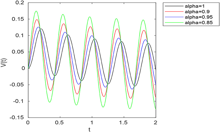
Figure 3. Graph of the voltage in the RC circuit for different values of α with μ(t) = sin(15t) and (a, b) = (1, 0).

FIGURE 4

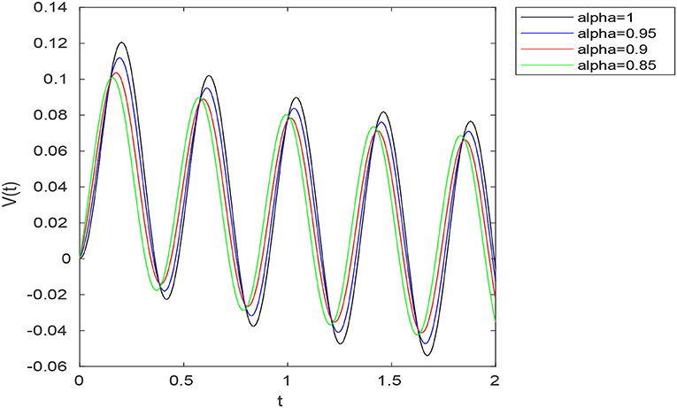
Figure 4. Graph of the voltage in the RC circuit for different values of α with μ(t) = sin(15t) and $(a, b) = (2, \sqrt{2})$ .

FIGURE 5

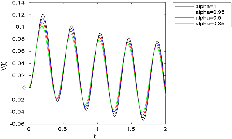
Figure 5. Graph of the voltage in the RC circuit for different values of α with μ(t) = sin(15t) and (a, b) = (10, 3).

8. Conclusion

In this contribution, we suggested a fractional derivative involving the kernel function

\begin{array}{r} k_{a, b} (t, s) = (\frac{1}{1 - α}) (\frac{a^{2} + b^{2}}{a}) e^{- \frac{a α (t - s)}{1 - α}} cos (\frac{b α (t - s)}{1 - α}), \\ a > 0, b \geq 0, 0 < α < 1 . \end{array}

In the particular case (a, b) = (1, 0), the above function reduces to Caputo-Fabrizio kernel. We studied fractional differential equations via this new concept in both theoretical and numerical aspects. In the theoretical point of view, we investigated the existence and uniqueness of solutions to non-linear fractional boundary value problems involving the new introduced fractional derivative. Namely, using Banach fixed point theorem, the existence and uniqueness of weak solutions to (5.7) was established under certain conditions imposed on the non-linear term F and the parameters a, b and α. In the numerical point of view, a numerical algorithm based on Picard iterations was proposed for solving the considered problem. Numerical experiments were provided using as a model example the fractional boundary value problem (6.1). In Figure 1, we presented the exact solution (u₁(t)) for α = 1 and numerical solutions z₁(t), z₃(t), and z₁₀(t) to (6.1) for α ∈ {0.95, 0.7}. One observes that for n = 10, z_n(t) is close enough to u₁(t), which confirms the convergence of the proposed algorithm. Finally, as application, we proposed a fractional model of an RC electrical circuit using the new introduced fractional derivative. One can compare the voltage V(t) obtained for different values of α in the Caputo-Fabrizio case (a, b) = (1, 0) (see Figure 3) with that obtained using different values of (a, b) (see Figures 4, 5). Namely, one can show that the voltage V(t) obtained with the use of the generalized fractional Caputo-Fabrizio derivative is more stable with respect to α than that obtained with the use of Caputo-Fabrizio fractional derivative.

Data Availability Statement

All datasets generated for this study are included in the article/supplementary material.

Author Contributions

All authors listed have made a substantial, direct and intellectual contribution to the work, and approved it for publication.

Funding

BS was supported by Researchers Supporting Project RSP-2019/4, King Saud University, Riyadh, Saudi Arabia.

Conflict of Interest

The authors declare that the research was conducted in the absence of any commercial or financial relationships that could be construed as a potential conflict of interest.

References

1. Frunzo L, Garra R, Giusti A, Luongo V. Modeling biological systems with an improved fractional Gompertz law. Commun Nonlinear Sci Num. (2019) 74:260–7. doi: 10.1016/j.cnsns.2019.03.024

CrossRef Full Text | Google Scholar

2. Gao W, Veeresha P, Prakasha D, Baskonus HM, Yel G. A powerful approach for fractional Drinfeld-Sokolov-Wilson equation with Mittag-Leffler law. Alex Eng J. (2019) 58:1301–11. doi: 10.1016/j.aej.2019.11.002

CrossRef Full Text | Google Scholar

3. Gao W, Yel G, Baskonus HM, Cattani C. Complex solitons in the conformable (2+1)-dimensional Ablowitz-Kaup-Newell-Segur equation. AIMS Math. (2020) 5:507–21. doi: 10.3934/math.2020034

CrossRef Full Text | Google Scholar

4. Jleli M, Kirane M, Samet B. A numerical approach based on ln-shifted Legendre polynomials for solving a fractional model of pollution. Math Methods Appl Sci. (2017) 40:7356–67. doi: 10.1002/mma.4534

CrossRef Full Text | Google Scholar

5. Qin S, Liu F, Turner I, Yang Q, Yu Q. Modelling anomalous diffusion using fractional Bloch-Torrey equations on approximate irregular domains. Comput Math Appl. (2018) 75:7–21. doi: 10.1016/j.camwa.2017.08.032

CrossRef Full Text | Google Scholar

6. Song F, Yang H. Modeling and analysis of fractional neutral disturbance waves in arterial vessels. Math Model Nat Phenom. (2019) 14:301. doi: 10.1051/mmnp/2018072

CrossRef Full Text | Google Scholar

7. Srivastava H, Gunerhan H. Analytical and approximate solutions of fractional-order susceptible-infected-recovered epidemic model of childhood disease. Math Methods Appl Sci. (2019) 42:935–41. doi: 10.1002/mma.5396

CrossRef Full Text | Google Scholar

8. Srivastava H, Saad K. Some new models of the time-fractional gas dynamics equation. Adv Math Model Appl. (2018) 3:5–17.

Google Scholar

9. Yang X, Machado J, Baleanu D. Exact traveling-wave solution for local fractional Boussinesq equation in fractal domain. Fractals. (2018) 25:1740006. doi: 10.1142/S0218348X17400060

CrossRef Full Text | Google Scholar

10. Yang X, Mahmoud A, Cattani C. A new general fractional-order derivative with Rabotnov fractional-exponential kernel applied to model the anomalous heat transfer. Therm Sci. (2019) 23:1677–81. doi: 10.2298/TSCI180825254Y

CrossRef Full Text | Google Scholar

11. Machado J, Kiryakova V, Mainardi F. Recent history of fractional calculus. Commun Nonlinear Sci Numer Simul. (2011) 16:1140–53. doi: 10.1016/j.cnsns.2010.05.027

CrossRef Full Text | Google Scholar

12. Caputo M, Fabrizio M. A new definition of fractional derivative without singular kernel. Progr Fract Differ Appl. (2015) 1:1–13. doi: 10.12785/pfda/010201

CrossRef Full Text | Google Scholar

13. Ali F, Saqib M, Khan I, Sheikh N. Application of Caputo-Fabrizio derivatives to MHD free convection flow of generalized Walters'-B fluid model. Eur Phys J Plus. (2016) 131:377. doi: 10.1140/epjp/i2016-16377-x

CrossRef Full Text | Google Scholar

14. Atangana A. On the new fractional derivative and application to nonlinear Fisher's reaction-diffusion equation. Appl Math Comput. (2016) 273:948–56. doi: 10.1016/j.amc.2015.10.021

CrossRef Full Text | Google Scholar

15. Bhatter S, Mathur A, Kumar D, Singh J. A new analysis of fractional Drinfeld–Sokolov–Wilson model with exponential memory. Phys A. (2020) 573:122578. doi: 10.1016/j.physa.2019.122578

CrossRef Full Text | Google Scholar

16. Caputo M, Fabrizio M. Applications of new time and spatial fractional derivatives with exponential kernels. Progr Fract Differ Appl. (2016) 2:1–11. doi: 10.18576/pfda/020101

CrossRef Full Text | Google Scholar

17. Gao F, Yang XJ. Fractional Maxwell fluid with fractional derivative without singular kernel. Therm Sci. (2016) 20:871–7. doi: 10.2298/TSCI16S3871G

CrossRef Full Text | Google Scholar

18. Gómez-Aguilar J, Yépez-Martinez H, Calderón-Ramón C, Cruz-Orduna I, Escobar-Jiménez R, Olivares-Peregrinoictor V. Modeling of a mass-spring-damper system by fractional derivatives with and without a singular kernel. Entropy. (2015) 17:6289–303. doi: 10.3390/e17096289

CrossRef Full Text | Google Scholar

19. Hristov J. Transient heat diffusion with a non-singular fading memory: from the Cattaneo constitutive equation with Jeffrey's kernel to the Caputo-Fabrizio time-fractional derivative. Therm Sci. (2016) 20:765–70. doi: 10.2298/TSCI160112019H

CrossRef Full Text | Google Scholar

20. Kumar D, Singh J, Al Qurashi ADB. A new fractional SIRS-SI malaria disease model with application of vaccines, antimalarial drugs, and spraying. Adv Differ Equat. (2019) 2019:278. doi: 10.1186/s13662-019-2199-9

CrossRef Full Text | Google Scholar

21. Kumar D, Singh J, Baleanu D, Sushila D. Analysis of regularized long-wave equation associated with a new fractional operator with Mittag-Leffler type kernel. Phys A. (2018) 492:155–67. doi: 10.1016/j.physa.2017.10.002

CrossRef Full Text | Google Scholar

22. Kumar D, Singh J, Tanwar K, Baleanu D. A new fractional exothermic reactions model having constant heat source in porous media with power, exponential and Mittag-Leffler laws. Int J Heat Mass Transf. (2019) 138:1222–7. doi: 10.1016/j.ijheatmasstransfer.2019.04.094

CrossRef Full Text | Google Scholar

23. Losada J, Nieto J. Properties of a new fractional derivative without singular kernel. Progr Fract Differ Appl. (2015) 1:87–92. doi: 10.12785/pfda/010202

CrossRef Full Text | Google Scholar

24. Singh J, Kumar D, Baleanu D. New aspects of fractional Biswas-Milovic model with Mittag-Leffler law. Math Model Nat Phenom. (2019) 14:303. doi: 10.1051/mmnp/2018068

CrossRef Full Text | Google Scholar

25. Atangana A, Baleanu D. New fractional derivative with non-local and non-singular kernel. Therm Sci. (2016) 20:757–63. doi: 10.2298/TSCI160111018A

CrossRef Full Text | Google Scholar

26. Gao W, Ghanbari B, Baskonus HM. New numerical simulations for some real world problems with Atangana-Baleanu fractional derivative. Chaos Solit Fract. (2019) 128:34–43. doi: 10.1016/j.chaos.2019.07.037

CrossRef Full Text | Google Scholar

27. Jarad F, Abdeljawad T, Hammouch Z. On a class of ordinary differential equations in the frame of Atangana-Baleanu fractional derivative. Chaos Solit Fract. (2019) 117:16–20. doi: 10.1016/j.chaos.2018.10.006

CrossRef Full Text | Google Scholar

28. Kumar D, Singh J, Baleanu D. On the analysis of vibration equation involving a fractional derivative with Mittag-Leffler law. Math Methods Appl Sci. (2019) 43:443–57. doi: 10.1002/mma.5903

CrossRef Full Text | Google Scholar

29. Singh J, Kumar D, Hammouch Z, Atangana A. A fractional epidemiological model for computer viruses pertaining to a new fractional derivative. Appl Math Comput. (2018) 316:504–15. doi: 10.1016/j.amc.2017.08.048

CrossRef Full Text | Google Scholar

30. Folland GB. Fourier Analysis and Its Applications. Providence, RI: American Mathematical Society (1992).

Google Scholar

31. Schiff J. The Laplace Transform: Theory and Applications. New York, NY: Springer (2013).

Google Scholar

32. Abramowitz M, Stegun I. Handbook of Mathematical Functions With Formulas, Graphs, and Mathematical Tables. New York, NY: Dover (1972).

Google Scholar

33. Gómez-Aguilar J, Razo-Hernández R, Granados-Lieberman D. A physical interpretation of fractional calculus in observables terms: analysis of the fractional time constant and the transitory response. Rev Mex Fis. (2014) 60:32–8.

Google Scholar

Keywords: fractional derivative, non-singular kernel, Picard iteration, RC-electrical circuit, convergence

Citation: Alshabanat A, Jleli M, Kumar S and Samet B (2020) Generalization of Caputo-Fabrizio Fractional Derivative and Applications to Electrical Circuits. Front. Phys. 8:64. doi: 10.3389/fphy.2020.00064

Received: 25 December 2019; Accepted: 28 February 2020;
Published: 20 March 2020.

Edited by:

Jagdev Singh, JECRC University, India

Reviewed by:

Haci Mehmet Baskonus, Harran University, Turkey
Devendra Kumar, University of Rajasthan, India

Copyright © 2020 Alshabanat, Jleli, Kumar and Samet. This is an open-access article distributed under the terms of the Creative Commons Attribution License (CC BY). The use, distribution or reproduction in other forums is permitted, provided the original author(s) and the copyright owner(s) are credited and that the original publication in this journal is cited, in accordance with accepted academic practice. No use, distribution or reproduction is permitted which does not comply with these terms.

*Correspondence: Sunil Kumar, skumar.math@nitjsr.ac.in

ORIGINAL RESEARCH article

Generalization of Caputo-Fabrizio Fractional Derivative and Applications to Electrical Circuits

1. Introduction

2. Some Preliminaries on Harmonic Analysis

3. Fractional Derivative With an Arbitrary Non-singular Kernel

4. A Generalized Caputo-Fabrizio Fractional Derivative

5. Applications to Fractional Differential Equations

6. Numerical Solution via Picard Iteration

7. Applications to RC Electrical Circuits

8. Conclusion

Data Availability Statement

Author Contributions

Funding

Conflict of Interest

References

This article is part of the Research Topic

People also looked at