Machine Learning for Automatic Classification of Tomato Ripening Stages Using Electrophysiological Recordings

Introduction

Ripening is a part of fruit development in which biochemical and physiological changes occur, making the fruit more attractive to seed dispersers and consumers (Prasanna et al., 2007; Corpas et al., 2018). As the fruit ripens, especially if it is fleshy, it becomes more palatable, soft, and colorful (there are exceptions, such as the avocado, which remains green). Intense metabolic activities are underlying these sensory changes, such as increased respiration, chlorophyll degradation, biosynthesis of carotenoids, anthocyanins, essential oils, and flavor and aroma components, increased activity of cell wall-degrading enzymes, modification in carbohydrate and organic acid profile, and a transient increase in ethylene production (Prasanna et al., 2007; Batista-Silva et al., 2018; Wang et al., 2018; Forlani et al., 2019).

Fleshy fruits are usually categorized in climacteric and non-climacteric, according to the ripening pattern in terms of respiratory rate and the production of the phytohormone ethylene (Pérez-Llorca et al., 2019). In climacteric fruits, there is an increase in respiratory rate accompanied by a peak in ethylene production. The fruits that present this pattern of ripeness can be harvested green, as this characteristic allows them to ripen detached from the plant. Non-climacteric fruits do not show an increase in respiration and ethylene synthesis, and generally the respiratory rate decreases as the ripening progresses. This type of fruit must end the ripening process connected to the plant (Corpas et al., 2018). Tomato (Solanum lycopersicum L.) is an example of climacteric fruit widely used as a model in research that involves ripening and ethylene signaling (Klee and Giovannoni, 2011).

The ripening process in tomatoes has different stages which are generally classified according to the color of the fruit's surface (López Camelo and Gómez, 2004; El-Bendary et al., 2015). The USDA (United States Department of Agriculture) has established standards for the classification of fresh tomatoes based on the external color of the fruit through visual appreciation. This system classifies fresh tomatoes into six categories, according to the approximate percentage of green color of the surface: green (100% green), breaker (there is a break in the color with lesser than 10% of other than green color), turning (10–30% of the surface is not green), pink (30–60% of the surface is not green), light red (60–90% of the surface is not green) and red (more than 90% of the surface is not green) (USDA, 2005).

It is worth mentioning that not all varieties of tomatoes undergo all these stages, and these transitions may not be easily visible to human eyes. In addition to the marked difference in color between the stages, which involves carotenoid synthesis and chlorophyll degradation in tomatoes, there are other characteristics of each stage. Regarding respiration and ethylene synthesis, the breaker stage is the one with a marked increase, with the exchange of system 1 of its synthesis for system 2, which is more intense and autocatalytic (Liu et al., 2015). The activation of enzymes related to fruit softening occurs in the early ripening stages. However, it becomes prominent in the later stages (Forlani et al., 2019). The activity of pectin methylesterase (PME), for example, increases as mature green tomatoes pass through different color stages to become full red. Unripe fruits are rich in PME, while ripe fruits are rich in hydrolase enzymes. Also, cell wall hydrolases show a pick of activity in the climacteric (Prasanna et al., 2007). The search for better classification strategies for fruit ripening stages is a constant target of research. This is important to determine the best harvesting point and thus avoid losses. Techniques with chlorophyll fluorescence induction (Abdelhamid et al., 2020) and Machine Learning (ML) using supervised training with images (El-Bendary et al., 2015) are some examples of targeted studies to monitoring and classifying ripening stages using different strategies.

All the physiological processes and biochemical alterations that occur during ripening can attribute to each stage “electrical signatures,” that arise from the movement of ions, electrons, and protons in the cells and tissues (de Toledo et al., 2019). In addition to classic hydraulic and chemical signals, such as phytohormones and reactive oxygen species (ROS), it is known that electrical signals perform several functions in plants (Białasek et al., 2017; Gao et al., 2019; Farmer et al., 2020; Volana Randriamandimbisoa et al., 2020). They are generated by the transient imbalance in membrane potential, caused by the influx/efflux of ions and H⁺ by ion channels, plasma membrane transporters and electrogenic pumps (Fromm and Lautner, 2007; Zimmermann et al., 2009; Sukhov et al., 2014; Vodeneev et al., 2016; de Toledo et al., 2019). Studies that focus on characteristics of individual signals from one or a few cells, such as action potentials (APs) and variation potentials (VPs), can underestimate the complexity of many overlapping electrical signals operating simultaneously, which creates a web of systemic information where multiple electrical signals are layered in time and space (De Loof, 2016; Souza et al., 2017; Debono and Souza, 2019). This is the “electrome,” i.e., the totality of ionic currents of any living entity, from the cell up to the whole organism level (De Loof, 2016). Thus, based on this general definition, the term “plant electrome” was proposed. It corresponds to the plants' bioelectrical activity measured as micro-voltage changes in stimulated or non-stimulated tissues (Saraiva et al., 2017; de Toledo et al., 2019).

Due to the high complexity of a typical plant electrome profile, ML techniques emerge as a powerful tool for data classification of plant electrophysiological recordings (Chatterjee et al., 2015; Pereira et al., 2018; Tran et al., 2019; Simmi et al., 2020; Parise et al., 2021; Reissig et al., 2021). ML is already being used in some potential applications in fruit ripening, but mostly in studies using images for training and ML classification (Taghadomi-Saberi et al., 2018; Vaviya et al., 2019; Alam Siddiquee et al., 2020; Cho et al., 2020). Several ML features for the classification of plant electrical signals, and their changes under different environmental stimuli, have already been successfully studied and employed (Chatterjee et al., 2015, 2018; Chen et al., 2016). The study developed by Souza et al. (2017) opened new possibilities to test new features for classification by ML in data as complex as the electrome of the plant. They proposed that the electrical signals captured in the plant can exhibit a self-organized critical state and complex non-linear behavior (Souza et al., 2017).

Considering the differences in the fruit physiology and the physicochemical processes underlying the changes at different ripening stages, it would be expected that the electrical activity would change accordingly. In this study, we propose the use of the fruit electrical activity, more precisely, the analysis of the electrome recordings as a source for parameters to support the classification of the ripening stages by ML techniques. Thus, the goal of this study was to differentiate tomato ripening stages using the fruit electrome as a feature for the training and classification of ML techniques.

Materials and Methods

Plant Material and Experimental Conditions

Seeds of cherry tomato (Solanum lycopersicum var. cerasiforme) were germinated in a polystyrene honeycomb germination box, filled with a commercial organic substrate (kept moist by spraying distilled water daily), where they remained for 7 days in a germinating chamber (25°C, photoperiod of 12 h). After this period, the seedlings were transplanted to 1.0 L plastic pots filled with commercial organic substrate. The tomato plants were grown in a greenhouse at the campus of Capão do Leão of the Federal University of Pelotas (31° 52′ 32″ S and 52° 21′ 24″ W, altitude 13 m). The average temperature in the greenhouse during the experimental period was 28.5 ± 12.9°C and the irradiance, from natural light, was on average 800 μmol photons m⁻² s⁻¹ (Reissig et al., 2018).

After transplantation, the plants were watered on alternate days (100 mL) and supplied with 50 mL of nutrient solution (Hoagland and Arnon, 1950) three times a week. When the fruits were green and fully established (before progressing to the breaker stage) they were harvested randomly from 50 tomato plants and transferred to laboratory conditions (25.0 ± 2.0°C, photoperiod of 12 h) where the experiment was carried on. In each essay, four fruits were placed in a Faraday's cage (Figure 1) and a pair of needle electrodes (EL452 model; Biopac Systems, Goleta, CA, EUA) were inserted 1 cm apart from each other (over the vascular bundles that were visible), 1 day before the signal recording, for acclimation. Five repetitions with four fruits each were made, totaling 20 fruit samples. The fruit ripening stages were categorized as follows: mature green (MG), breaker (BR) and light red (LR) (Gonzalez et al., 2015; Reissig et al., 2020). We recorded the fruits' electrome while they transitioned through all the ripening stages, from MG to LR. Consequently, the electrome of each replicate refers to the MG, BR, and LR of the same fruits. The bioelectrical signals were acquired during the fruit ripening in data acquisitions throughout 24 h until all fruits were in the LR stage.

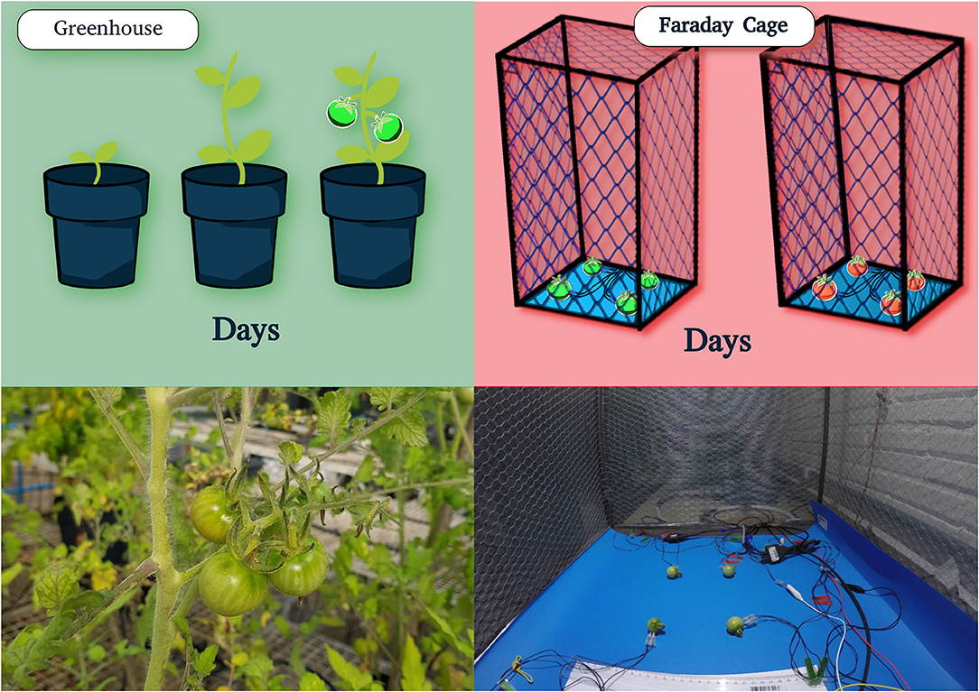
Figure 1. Experimental scheme of plant growth and experimental setup. Tomato plants were grown in greenhouse until fruit reach mature green (MG) ripening stage (upper left quadrant). Illustration of cherry tomato fruit vine (lower left quadrant). MG fruit was harvested and transported to the electrophysiology room, where it was placed in a Faraday's cage and a pair of electrode was inserted in each fruit, totaling four per replicate. The recording of electrical signals through ripening stages were conducted in the same fruit placed initially (upper right quadrant). Illustration of fruit's electrophysiological measures in a Faraday's cage (lower right quadrant).

Data Acquisition

Electrical signals were recorded with the electronic system for data acquisition MP36 (Biopac Systems, Goleta, CA, EUA), composed of four channels with high input impedance (10 GΩ). The signals were acquired by fixing a sampling rate of f_s = 62.5 Hz with two filters, one high-pass (0.5 Hz cut-off frequency) and the other low-pass (1.5 kHz cut-off frequency). The bioelectrical runs were analyzed as voltage variation (μV) time series ΔV = {ΔV₁, ΔV₂, …, ΔV_N} in which ΔV_i is the difference of potential between the inserted electrodes, scored in each $\frac{1}{f_s}$ time interval, and N is the total length of the series. Also, one pair of electrodes was left open throughout all the essays as a control of the environment. An open electrode is a reference, i.e., a pair of electrodes not connected to the plants left inside the Faraday cage that records environmental noise and noise intrinsic to the equipment. For the open electrodes, the signals remained stable throughout the period, showing that the variation in signal complexity was not due to the equipment. Open electrode signals show a typical Gaussian noise with a lower amplitude than the plant signal baseline (Saraiva et al., 2017). Beyond visual inspection (see Supplementary Figure 1), the time series were analyzed with different methods to characterize the temporal dynamics of the signals during the transition of the ripening stages of tomato fruits.

Data Analyses and Machine Learning Classification Methods

Feature's Acquisition

For the ML analyses, each time series (TS) was split into 10 interchangeable parts, with a lag of 30%. This is a necessary procedure for increasing the sample size. In the end, a total of 1,480 overlapping time series were obtained (Pereira et al., 2018). They were divided into three classes: Class MG (Mature Green) with 470 samples; Class BR (Breaker) with 490 samples; Class LR (Light Red) with 520 samples.

All the calculations and data processing applied to the time series analyses were performed in Python (Van Rossum and Drake, 2009). The code libraries used were: Numpy (Harris et al., 2020) and Pandas (McKinney, 2010) for data manipulation; Scipy, Obspy, and Math for mathematical calculations; Matplotlib for creating graphics; Sklearn and Statsmodels for machine learning (Pedregosa et al., 2020; Virtanen et al., 2020).

Afterwards, the approximate entropy (ApEn), Fourier transform (FFT), Power Spectral Density (PSD), and Wavelets were calculated for each sample. The FFT decomposes the time series data into a combination of signals of different frequencies, allowing to verify which frequencies are noise and which are data. Since the electrophysiological series is the sum of multiple frequencies, PSD was calculated. Thus, it is possible to obtain the power that each frequency produces in the density of the signal spectrum. It helps to observe the frequencies of the stochastic process and the periodicities of events, as well as the description of the energy distributed by each frequency of the signal. The Wavelet analysis gives information about these frequencies in the domain of time, that is, when and for how long specific frequencies occur. The ApEn gives information about the complexity of the signal, using the patterns found in the time series (Shannon, 1948; Kolmogorov, 1956; Pincus, 1995; Delgado-Bonal and Marshak, 2019). In other words, low ApEn values indicate a low level of complexity, and their patterns tend to be repetitive and predictable. High ApEn values indicate a higher level of complexity, and the patterns are more difficult to predict. The procedures for calculating ApEn (Figure 2) were based on the original theory of Pincus (1991). For FFT analysis we used the set of SciPy libraries (Virtanen et al., 2020) using Bluestein's algorithm (Bluestein, 1970). The PSD was calculated through the SciPy library using Welch's method (Welch, 1967), and Wavelets through the PyWavelets library (Lee et al., 2019) with the Discrete Wavelet Transform (DWT) method, having as family Daubechies wavelets (Daubechies, 1992).

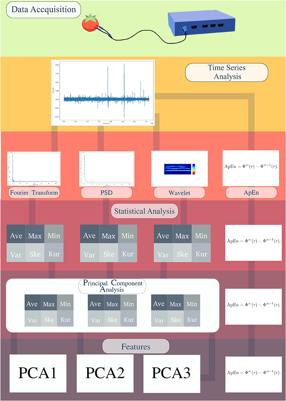
Figure 2. Scheme representing the acquisition of features for Machine Learning analysis. Fruit electrical signals were recorded with an electronic system for data acquisition (MP36). The bioelectrical runs were analyzed as voltage variation (μV) time series (TS). Afterwards, the approximate entropy (ApEn), Fourier transform (FFT), Power Spectral Density (PSD), and Wavelets were calculated. Except for ApEn, the descriptive analyzes of average, maximum value, minimum value, variance, skewness, and kurtosis were calculated. With these results, PCA was calculated and PCA1, PCA2, and PCA3 obtained. Finally, we obtained three PCAs and ApEn as ML features.

The average, maximum value, minimum value, variance, skewness, and kurtosis were calculated for FFT, PSD and Wavelets. With these results, a Principal Component Analysis (PCA) was calculated, resulting in three principal components (PCA1, PCA2, and PCA3). Together with the three PCAs, ApEn was used as an additional ML feature (Figure 2). Before defining the four features previously mentioned, tests with n-dimensions were performed (n = 2–19). The use of four dimensions was the one that obtained the best cost-benefit trade-off between accuracy and time of computational execution. PCA is a linear dimensionality reduction technique that can be used to extract information from a high-dimensional space, projecting it into a smaller subspace and preserving essential parts that have more variation in the data, and also removes the non-essential parts with less variation (Wold et al., 1987).

ML Training and Testing

We separated the two datasets, one for training the ML and the other for effectively testing our data. To avoid the problem of Underfitting or Overfitting (Jabbar and Khan, 2014), and to obtain a more reliable result, we used the Stratified KFold (n_splits = 4 and shuffle = True) and Cross Validate (k = 10) methods (Forman and Scholz, 2010; Adagbasa et al., 2019). This cross-validation object divides the data into k-folds, ensuring that each fold is an appropriate representative of the data, both in an equal division between classes, as well as keeping each round of training and testing pure in terms of repeating the same samples. This division is done as a percentage, and we used n_splits = 4 (Mohri et al., 2018).

Considering different configurations of training and test groups, the possibility of chance interference in our results was reduced. A prior evaluation of the datasets was made, and the analysis of the ripening stages BR vs. MG was subjected to several loops, leading to thousands of different parameter combinations. After this analysis, the hyperparameters that obtained the best levels of accuracy were maintained for all subsequent analyzes (described together with each ML model).

In order to standardize random methods, we used the function numpy.random.seed with seed = 42. Considering the hypothesis of finding a difference between the ripening stages, we use several ML models to obtain the best one for each dataset, as the objective is to detect which groups of data can be better classified and determine the best accuracy or method in general. In a nutshell, we are interested in the individual classification of each class, and not in the best method used to achieve this, maintaining the information of which model was used only for the reproducibility of the experiment. The models used were chosen because they have different classification approaches and, with that, we intend to eliminate this variable from our study. The ML models used were:

Decision Tree (Hyperparameters: max_depth = 10 and min_samples_leaf = 64): it is a predictive model that uses a decision tree to go from observations about an item to conclusions about the item's target value. In decision analysis, a decision tree can be used to represent decision making visually and explicitly (Breiman et al., 1984).

SVC (Hyperparameters: max_iter = 100.000 and tol = 1e−1): Support Vector Classification is derived from SVM (Support Vector Machine). They are associated with supervised learning models that use classification and regression analysis. An SVM training algorithm builds a model that assigns new examples to one category or another, making it a non-probabilistic binary linear classifier (Chang and Lin, 2020).

Linear SVC (Hyperparameters: max_iter = 100.000 and tol = 1e−1): it is similar to SVC, but it has more flexibility in the choice of penalty and loss functions and should be better sized for a large number of samples. This class supports sparse and dense entries (Hsu et al., 2016).

Gaussian Process (Hyperparameters: max_iter_predict = 150 and multi_class = one_vs_one for analyzes with two classes and one_vs_rest for 3-class analysis): implements Gaussian Processes (GP) for regression purposes. The GP is a generic method of supervised learning, designed to solve problems of regression and probabilistic classification (Mackay and Gibbs, 2000).

KNeighbors [Hyperparameters: n_neighbors = (2 for two-class analysis and 3 for 3-class analysis), algorithm = kdtree and leaf_size = 50]: In pattern recognition, the nearest k-neighbors algorithm (k-NN) is a non-parametric method used for classification and regression. In both cases, the entry consists of the k closest training examples in space (Maillo et al., 2017).

Random Forest (Hyperparameters: n_estimators = 200, max_depth = 5, and min_samples_leaf = 128): it is a joint learning method for classification and regression that operates by building several decision trees at the time of training and generating the class of individual trees. Decision forests correct the habit of decision trees adjusting to their training set (Maillo et al., 2017).

Gaussian NB (Hyperparameters: var_smoothing = 1e−7): In machine learning, Bayes' naïve classifiers are a family of simple “probabilistic classifiers” based on the application of Bayes' theorem. This method is easier to solve the problem of judging classes as belonging to one category or another (Chan et al., 1982).

The Dummy Classifier method was used as the control. It uses several unintelligent strategies to classify data. Based on the returned accuracy, we obtain a standard for comparison. A model that obtains a low accuracy, similar to the Dummy, shall not be considered suitable for the database used (sklearn.dummy.DummyClassifier, 2020). The strategies used by the Dummy Classifier are:

• Dummy Stratified: Sort the data in a randomly stratified way;

• Dummy Most Frequent: Assume that all test data belong to the most frequent class in training;

• Dummy Prior: Classifies the data giving priority to a specific class;

• Dummy Constant (constant = number of classes−1): Assumes a constant value passed previously.

Precision, Sensitivity, and F1-Score

In order to be able to infer results about a specific class, such as asking whether class X is easier to classify than class Y, an analysis of individual visualization metrics was performed using Precision, Sensitivity and F1-score.

Sensitivity

For all cases classified as positive, which value among the informed positives was correct?

A perfect classification would return 1, that is, all the ML classification was correct (Powers, 2020; Tharwat, 2021).

Precision

For all instances that have been rated as positive, what is the value of true positive?

A perfect classification would return 1, that is, ML correctly classified all members of the class.

F1-Score

The F1-score is the harmonic mean of Precision and Sensitivity, where an F1 score reaches its best value in 1 (perfect precision and sensitivity) (Van Rijsbergen, 1979).

The scheme for calculating Precision, Sensitivity and F1-score can be found in Figure 3.

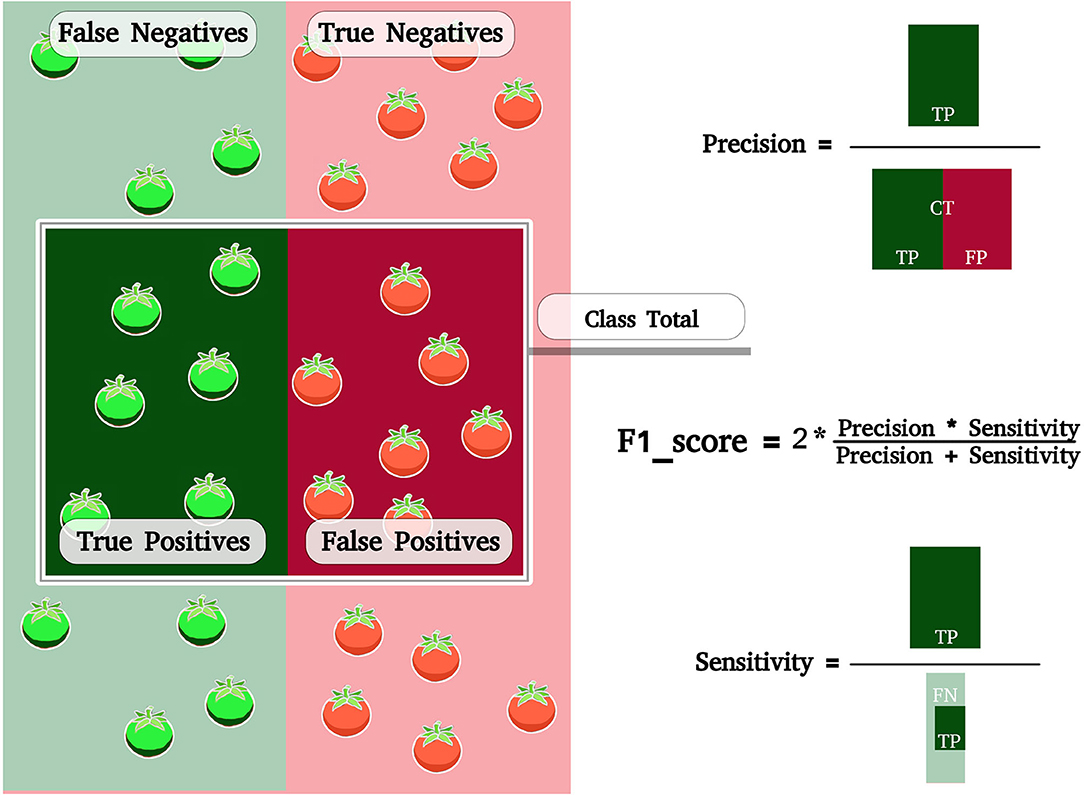
Figure 3. Scheme representing the sample space submitted to ML classification. Class Total is the region where the ML has classified green. The green tomatoes within the classification region are correct. Red tomatoes within the region were classified as non-red. A true positive is a result where the model correctly predicts the class. A false positive is a result where the model incorrectly predicts the class. A false negative is when the model incorrectly predicts the wrong class. CT, Class Total; TP, True Positives; FP, False Positives; FN, False Negatives.

The calculation of the F1-score provides the information about which class is better classified, that is, which class has features better identified by ML. In the present work, this corresponds to say that the time series of some ripening stage carries enough information to be distinct.

To identify the relationship between the ripening stages, the analyses were carried out, group by group and all together. Thus, the groups were MG × BR, BR × LR, and MG × BR × LR. In this manner, it is possible to verify whether each group has unique characteristics that would differentiate them when compared with the other groups.

Results

In general, the ML methods tested to classify between different ripening stages were successful when compared with the performance of the Dummy test, which is the control here. For instance, the Random Forest method reached an accuracy of 80.76% in distinguishing between MG (Mature Green) and BR (Breaker) ripening stages, while the Dummy test barely reached a random choice (53.64% of accuracy) (Figure 4A).

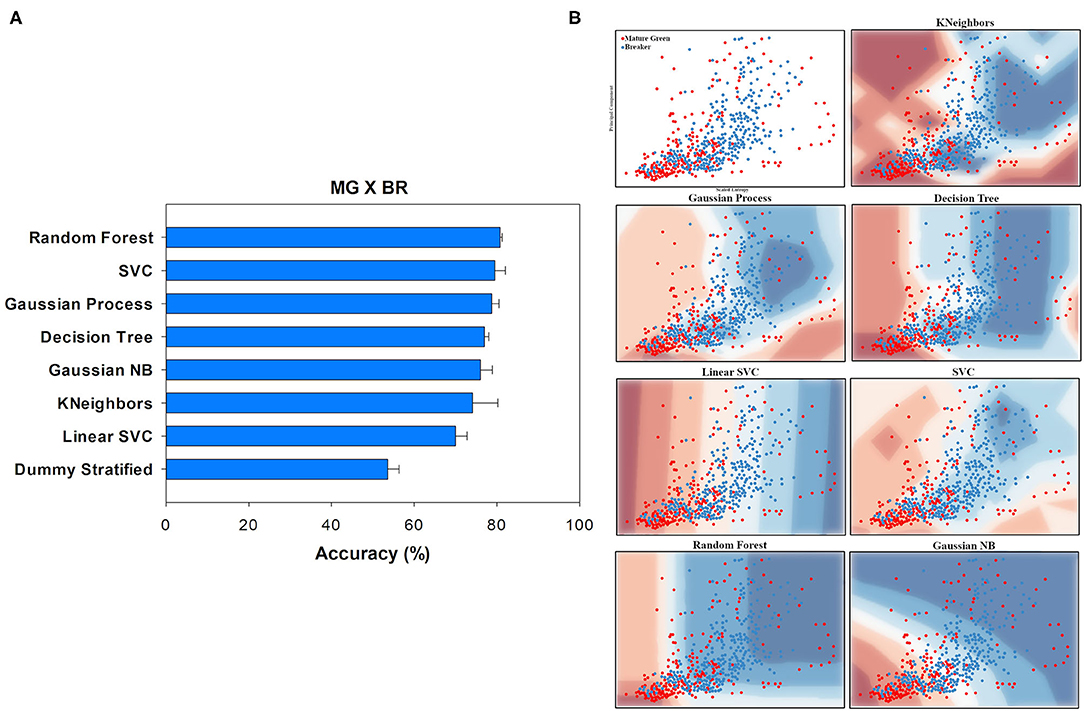
Figure 4. Accuracy (%) and standard deviation (A) of the Machine Learning models used to classify Mature Green (MG) and Breaker (BR) classes. Scatter plots (B) showing a sample space plan used in ML training for the MG × BR distribution. Red dots: MG; blue dots: BR. The regions are the demarcations made by ML to indicate levels of certainty of classification. The more reddish it is, the more certain it belongs to the MG group. The more bluish it is, the more certain it belongs to the BR group. The subtitle of each graph indicates the method used. On the y-axis is the data from PCA1. On the x-axis is the distribution of the Scaled Entropy.

The two-dimensional scatter plot for the features used in the classification is shown in the first graphs in Figure 4B. In this plot, it is possible to have a first picture of how the data were distributed. On the y-axis are the data from PCA1 and the distribution of the entropy value is on the x-axis. Both MG and BR ripening stages tended to be concentrated in the lower left quadrant. However, it can be observed that the BR stage showed a more linear trend with increasing entropy, while MG samples tended to spread across the chart plane. Although this information, at first glance, may not seem to be physiologically relevant, it was a relevant factor for ML classification.

The other graphics in Figure 4B show the decision-making graphs for the models used in the classification. Most models have classified the BR class (blue dots) with priority. This can be seen through the Sensitivity analysis (Table 1). Moreover, both classes showed similar Precision scores (0.74 for the MG and 0.78 for the BR), indicating that a part of the samples was too similar, making ML classification confuse. However, the Sensitivity of 0.62 for MG and 0.86 for BR indicated that ML was more successful in classifying BR, resulting in a higher F1-score.

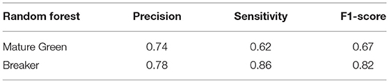
Table 1. Precision, Sensitivity, and F1-score of the Random Forest model to Mature Green and Breaker classification.

The ML classification, allowing a distinction between BR (Breaker) and LR (Light Red) ripening stages, showed 79.11% accuracy using the Random Forest algorithm, while the Dummy test reach barely 56.09%. Even considering the margin of error, ML managed to classify the groups with accuracy (Figure 5A).

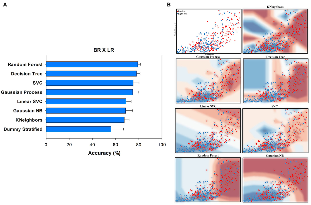
Figure 5. Accuracy (%) and standard deviation (A) of the Machine Learning models used to classify Breaker (BR) and Light Red (LR) classes. Scatter plots (B) showing a sample space plan used in ML training for the BR × LR distribution. Red dots: BR; blue dots: LR. The regions are the demarcations made by ML to indicate levels of certainty of classification. The more reddish it is, the more certain it belongs to the BR group. The more bluish it is, the more certain it belongs to the LR group. The subtitle of each graph indicates the method used. On the y-axis is the data from PCA1. On the x-axis is the distribution of the Scaled Entropy.

It was possible to notice that, although the data have a similar dispersion (Figure 5B), entropy was an important feature to improve the differentiation between the ripening stages. The groups are distinguished in the upper right and bottom left quadrants. However, several points remain in the center. The quadrants may have influenced the Precision values (BR 0.77 and LR 0.78) (Figure 5B). ML was more efficient in classifying the BR class, which can be seen by Sensitivity (BR 0.82 and LR 0.72). In the end, the BR stage obtained an F1-score of 0.79 against 0.74 of the LR stage, once again the best-classified instance (Table 2).

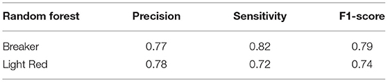
Table 2. Precision, Sensitivity, and F1-score of the Random Forest model to Breaker and Light Red classification.

When the three ripening stages (Mature Green × Breaker × Light Red) were analyzed together, less accuracy was observed compared to the analysis in pairs. The highest accuracy was 74.41% reached by the SVC algorithm, while the Dummy test exhibited an accuracy of only 42.45% (Figure 6A). This classification is more complex than a binary classification. It is possible to see how each group's data overlap (Figure 6B), mainly in the lower left quadrant, which resulted in less accuracy between the three classification groups. However, when analyzing the F1-score (Table 3), the BR group obtained a higher value, which demonstrates that the BR group is again better classified among the three stages.

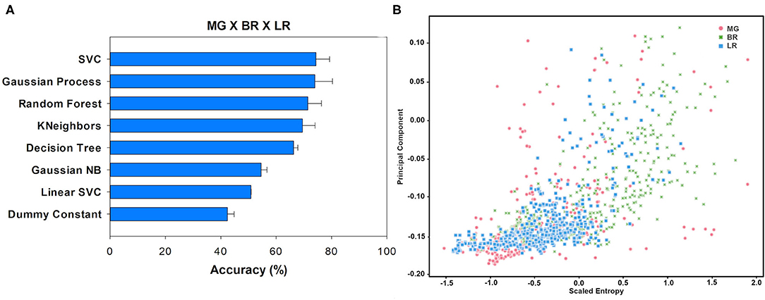
Figure 6. Accuracy (%) and standard deviation (A) of the Machine Learning models used to classify Mature Green (MG), Breaker (BR), and Light Red (LR) classes. Scatter plot (B) showing PCA1 and Scaled Entropy distribution (Mature Green × Breaker × Light Red). Red dots: MG; green dots: BR; blue dots: LR. On the y-axis is the data from PCA1. On the x-axis is the distribution of the Scaled Entropy.

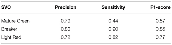
Table 3. Precision, Sensitivity, and F1-score of the SVC model to Mature Green, Breaker, and Light Red classification.

To summarize, the binary groups were the ones that obtained the best accuracy, especially the classification between MG and BR (Figures 4A,B). The analysis among the three groups showed the lowest accuracy. There is a discussion about the analysis of groups One-vs.-All and One-vs.-One (Binary classification vs. Multi-class classification) that are completely dependent on the method used for the classification (Bishop, 2006). As we use several methods, the fact that we found a low accuracy value when using the One-vs.-All technique indicates a difficulty for ML in classifying these groups. Regarding the F1-score, the BR stage showed the highest values in all comparison groups (Table 3).

Discussion

The results from the classification of ripening stages by ML techniques showed a more accurate distinction between MG (Mature Green) and Breaker (BR) than between BR and Light Red (LR) stages, indicating that BR and LR stages are more similar between them than MG and BR. In fact, the BR ripening stage was the most differentiable when analyzing the F1-score information (Table 3), with higher values in all classification groups. Physiologically, this result seems quite reasonable because the fruits at the MG stage have not yet started the ripening process effectively. On the other hand, tomatoes in BR and LR stages share more similarities regarding the physicochemical and biochemical processes underlying the ripening process. The increment in respiration and autocatalytic ethylene synthesis occurs in both BR and LR stages (Liu et al., 2015). Moreover, chlorophyll degradation, carotenoids accumulation, and cell wall lysis are other examples of common processes between both these stages.

Different physiological processes during ripening could affect the bioelectrical activity of the fruits causing the changes in the electrome detected by the ML analyses performed here. Increased respiration in climacteric fruits, accompanied by an increase in ethylene synthesis, can lead to an increase in reactive oxygen and ATP species (Brady, 1987; Decros et al., 2019). The latter can induce ATPases activation (Azevedo et al., 2008), which can affect ionic imbalance across cellular membranes, resulting in changes in membrane potential, which leads to the generation of electrical signals.

In addition, changes that occur in the cell wall during ripening can also lead to a characteristic “signature” of the electrical signals during the process. Pectin can form structures known as “egg box,” where the divalent calcium ion forms homogalacturonan cross-linked chains, leading to the strengthening of the gel matrix, regardless of any cellulose-pectin interaction. Later on, when the pectin is being demethylated and solubilized, the calcium ions are released from the structure (Aghdam et al., 2012; Wang et al., 2018). The calcium released in the process might affect the electrical pattern of the fruit as it ripens. Many other processes involved in ripening can lead to the generation of electrical signals with characteristic patterns. Plant electrophysiology is a field that still has a lot to be discovered, and studies focused on the electrophysiology of ripening are of great importance for a better understanding of this phenomenon.

Considering the impartiality of ML models, it was observed that the BR stage was used as a reference for the classifications. Basically, the classification models, for the most part, used the BR group as the one to be indicative of decision-making, a fact demonstrated in the results of Precision and Sensitivity. This result is also important to corroborate our hypothesis that the electrome of the tomato fruit in the BR stage is more classifiable than the MG and LR stages.

Several studies in the field of plant electrophysiology are demonstrating the potential practical uses of plant electrical signaling (Reissig et al., 2021). For instance, Tran et al. (2019) proposed the electrophysiological evaluation of tomato plants status using supervised machine learning. The methodology and electrophysiological sensor developed allowed the measurement of real-time electrical signals related to the plant water status in the field, without a Faraday cage. Another recent study showed the possibility of using the analysis of the plant's electrome to perform an early diagnosis of pathogenic fungi in tomatoes (Simmi et al., 2020). In both cases, machine learning techniques were used as an important tool to determine and classify changes in the plant's electrical signals. Therefore, automated techniques used in the harvest and the post-harvest can be increasingly improved with the use of ML.

Ji et al. (2020) have referred to the difficulty of automating and mechanizing the harvest of green peppers due to the similarity of the fruit color with the background and its form with the shape of the leaf. It is supposed that ML's multidimensional view could provide better results. The use of different features beyond images is an option to add more information layers to improve ML results. Our results have shown that electrophysiological analysis of plants can be used for this purpose. For example, ML could be trained for relating pictures of the fruit ripening stages to the electrome at each point. This first process can create a much more precise classification of ripening, possibly far beyond the stages described in the literature. At the dawn of the digital era, we can perfectly envisage machine learning as a fundamental part of sustainable agriculture and post-harvest technology. The path for it is just open.

Conclusion

The electrical signals underlying the physiological processes that occur at different ripening stages have different characteristics specific to each ripening stage. The high accuracy results obtained with unsupervised ML classification of the electrical signals from different ripening stages can open many opportunities for application in the automation of fruit harvesting. By combining our approach with data from hyperspectral images during fruit ripening, likely, it will be possible to reach even higher accuracy to determine specific targets for automatic harvesting in the near future.

Data Availability Statement

The original contributions presented in the study are included in the article/Supplementary Material, further inquiries can be directed to the corresponding author/s.

Author Contributions

GR: conceptualization, methodology, formal analysis, investigation, data curation, and writing—original draft preparation. TO: formal analysis, investigation, data curation, and writing—original draft preparation. ÁC: investigation, methodology, and data curation. AP: methodology and writing—reviewing and editing. DP: data curation and writing—reviewing and editing. GS: resources, writing—reviewing and editing, and supervision. All authors contributed to the article and approved the submitted version.

Funding

This study was supported in part by the Coordenação de Aperfeiçoamento de Pessoal de Nível Superior, Brazil (CAPES), Finance Code 001. Authors are also grateful to Conselho Nacional de Desenvolvimento Científico e Tecnológico (CNPq) for the financial support provided (401722/2016-3). GS was CNPq fellow (302715/2018-5).

Conflict of Interest

The authors declare that the research was conducted in the absence of any commercial or financial relationships that could be construed as a potential conflict of interest.

Publisher's Note

All claims expressed in this article are solely those of the authors and do not necessarily represent those of their affiliated organizations, or those of the publisher, the editors and the reviewers. Any product that may be evaluated in this article, or claim that may be made by its manufacturer, is not guaranteed or endorsed by the publisher.

Supplementary Material

The Supplementary Material for this article can be found online at: https://www.frontiersin.org/articles/10.3389/fsufs.2021.696829/full#supplementary-material

Supplementary Figure 1. Time series of electrical signals acquired during ripening process of cherry tomatoes. (A) Mature green fruit, (B) breaker fruit, (C) light red fruit. volt [ΔV (mV)] by time (seconds).

References

Abdelhamid, M. A., Sudnik, Y., Alshinayyin, H. J., and Shaaban, F. (2020). Non-destructive method for monitoring tomato ripening based on chlorophyll fluorescence induction. J. Agric. Eng. 52:1098. doi: 10.4081/jae.2020.1098
Adagbasa, E. G., Adelabu, S. A., and Okello, T. W. (2019). Application of deep learning with stratified K-fold for vegetation species discrimation in a protected mountainous region using Sentinel-2 image. Geocarto Int. doi: 10.1080/10106049.2019.1704070. [Epub ahead of print].
Aghdam, M. S., Hassanpouraghdam, M. B., Paliyath, G., and Farmani, B. (2012). The language of calcium in postharvest life of fruits, vegetables and flowers. Sci. Hortic. 144, 102–115. doi: 10.1016/j.scienta.2012.07.007
Alam Siddiquee, K. N., e, Islam, M. S., Dowla, M. Y. U., Rezaul, K. M., and Grout, V. (2020). Detection, quantification and classification of ripened tomatoes: a comparative analysis of image processing and machine learning. IET Image Process. 14, 2442–2456. doi: 10.1049/iet-ipr.2019.0738
Azevedo, I. G., Oliveira, J. G., da Silva, M. G., Pereira, T., Corrêa, S. F., Vargas, H., et al. (2008). P-type H+-ATPases activity, membrane integrity, and apoplastic pH during papaya fruit ripening. Postharvest Biol. Technol. 48, 242–247. doi: 10.1016/j.postharvbio.2007.11.001
Batista-Silva, W., Nascimento, V. L., Medeiros, D. B., Nunes-Nesi, A., Ribeiro, D. M., Zsögön, A., et al. (2018). Modifications in organic acid profiles during fruit development and ripening: correlation or causation? Front. Plant Sci. 9:1689. doi: 10.3389/fpls.2018.01689
Białasek, M., Górecka, M., Mittler, R., and Karpiński, S. (2017). Evidence for the involvement of electrical, calcium and ROS signaling in the systemic regulation of non-photochemical quenching and photosynthesis. Plant Cell Physiol. 58, 207–215. doi: 10.1093/pcp/pcw232
Bishop, C. (2006). Pattern Recognition and Machine Learning. EAI/Springer Innovations in Communication and Computing. New York, NY: Springer-Verlag.
Bluestein, L. (1970). A linear filtering approach to the computation of discrete Fourier transform. IEEE Trans. Audio Electroacoust. 18, 451–455. doi: 10.1109/TAU.1970.1162132
Brady, C. J. (1987). Fruit ripening. Annu. Rev. Plant Physiol. 38, 155–178. doi: 10.1146/annurev.pp.38.060187.001103
Breiman, L., Friedman, J., Stone, C. J., and Olshen, R. A. (1984). Classification and Regression Trees. Chapman and Hall/CRC. Available online at: https://www.routledge.com/Classification-and-Regression-Trees/Breiman-Friedman-Stone-Olshen/p/book/9780412048418 (accessed March 21, 2021).
Chan, T. F., Golub, G. H., and LeVeque, R. J. (1982). “Updating formulae and a pairwise algorithm for computing sample variances,” in COMPSTAT 1982 5th Symposium Held at Toulouse 1982, eds. H. Caussinus, P. Ettinger, and R. Tomassone (Physica; Heidelberg), 30–41.
Chang, C.-C., and Lin, C.-J. (2020). LIBSVM – A Library for Support Vector Machines. Available online at: https://www.csie.ntu.edu.tw/~cjlin/libsvm/ (accessed August 30, 2020).
Chatterjee, S., Malik, O., and Gupta, S. (2018). Chemical sensing employing plant electrical signal response-classification of stimuli using curve fitting coefficients as features. Biosensors 8:83. doi: 10.3390/bios8030083
Chatterjee, S. K., Das, S., Maharatna, K., Masi, E., Santopolo, L., Mancuso, S., et al. (2015). Exploring strategies for classification of external stimuli using statistical features of the plant electrical response. J. R. Soc. Interface 12:20141225. doi: 10.1098/rsif.2014.1225
Chen, Y., Zhao, D.-J., Wang, Z.-Y., Wang, Z.-Y., Tang, G., and Huang, L. (2016). Plant electrical signal classification based on waveform similarity. Algorithms 9:70. doi: 10.3390/a9040070
Cho, B.-H., Koyama, K., Olivares Díaz, E., and Koseki, S. (2020). Determination of “Hass” avocado ripeness during storage based on smartphone image and machine learning model. Food Bioprocess Technol. 13, 1579–1587. doi: 10.1007/s11947-020-02494-x
Corpas, F. J., Freschi, L., Rodríguez-Ruiz, M., Mioto, P. T., González-Gordo, S., and Palma, J. M. (2018). Nitro-oxidative metabolism during fruit ripening. J. Exp. Bot. 69, 3449–3463. doi: 10.1093/jxb/erx453
Daubechies, I. (1992). Ten Lectures on Wavelets. Philadelphia, PA: Society for Industrial and Applied Mathematics.
De Loof, A. (2016). The cell's self-generated “electrome”: the biophysical essence of the immaterial dimension of Life? Commun. Integr. Biol. 9:e1197446. doi: 10.1080/19420889.2016.1197446
de Toledo, G. R. A., Parise, A. G., Simmi, F. Z., Costa, A. V. L., Senko, L. G. S., Debono, M.-W., et al. (2019). Plant electrome: the electrical dimension of plant life. Theor. Exp. Plant Physiol. 31, 21–46. doi: 10.1007/s40626-019-00145-x
Debono, M.-W., and Souza, G. M. (2019). Plants as electromic plastic interfaces: a mesological approach. Prog. Biophys. Mol. Biol. 146, 123–133. doi: 10.1016/j.pbiomolbio.2019.02.007
Decros, G., Baldet, P., Beauvoit, B., Stevens, R., Flandin, A., Colombié, S., et al. (2019). Get the balance right: ROS homeostasis and redox signalling in fruit. Front. Plant Sci. 10:1091. doi: 10.3389/fpls.2019.01091
Delgado-Bonal, A., and Marshak, A. (2019). Approximate entropy and sample entropy: a comprehensive tutorial. Entropy 21:541. doi: 10.3390/e21060541
El-Bendary, N., El Hariri, E., Hassanien, A. E., and Badr, A. (2015). Using machine learning techniques for evaluating tomato ripeness. Expert Syst. Appl. 42, 1892–1905. doi: 10.1016/j.eswa.2014.09.057
Farmer, E. E., Gao, Y.-Q., Lenzoni, G., Wolfender, J.-L., and Wu, Q. (2020). Wound and mechanostimulated electrical signals control hormone responses. New Phytol. 227, 1037–1050. doi: 10.1111/nph.16646
Forlani, S., Masiero, S., and Mizzotti, C. (2019). Fruit ripening: the role of hormones, cell wall modifications, and their relationship with pathogens. J. Exp. Bot. 70, 2993–3006. doi: 10.1093/jxb/erz112
Forman, G., and Scholz, M. (2010). Apples-to-apples in cross-validation studies. ACM SIGKDD Explor. Newsl. 12, 49–57. doi: 10.1145/1882471.1882479
Fromm, J., and Lautner, S. (2007). Electrical signals and their physiological significance in plants. Plant Cell Environ. 30, 249–257. doi: 10.1111/j.1365-3040.2006.01614.x
Gao, Q., Xiong, T., Li, X., Chen, W., and Zhu, X. (2019). Calcium and calcium sensors in fruit development and ripening. Sci. Hortic. 253, 412–421. doi: 10.1016/j.scienta.2019.04.069
Gonzalez, C., Ré, M. D., Sossi, M. L., Valle, E. M., and Boggio, S. B. (2015). Tomato cv. 'Micro-Tom' as a model system to study postharvest chilling tolerance. Sci. Hortic. 184, 63–69. doi: 10.1016/j.scienta.2014.12.020
Harris, C. R., Millman, K. J., van der Walt, S. J., Gommers, R., Virtanen, P., Cournapeau, D., et al. (2020). Array programming with NumPy. Nature 585, 357–362. doi: 10.1038/s41586-020-2649-2
Hoagland, D. R., and Arnon, D. I. (1950). Preparing the nutrient solution. Water-Culture Method Grow. Plants Without Soil 347, 1–39.
Hsu, C.-W., Chang, C.-C., and Lin, C.-J. (2016). A Practical Guide to Support Vector Classification. Taipei: National Taiwan University. Available online at: https://www.csie.ntu.edu.tw/~cjlin/papers/guide/guide.pdf (accessed April 6, 2021).
Jabbar, H. K., and Khan, R. Z. (2014). “Methods to avoid over-fitting and under-fitting in supervised machine learning (comparative study),” in Computer Science, Communication and Instrumentation Devices (Singapore: Research Publishing Services), 163–172.
Ji, W., Gao, X., Xu, B., Chen, G., and Zhao, D. (2020). Target recognition method of green pepper harvesting robot based on manifold ranking. Comput. Electron. Agric. 177:105663. doi: 10.1016/j.compag.2020.105663
Klee, H. J., and Giovannoni, J. J. (2011). Genetics and control of tomato fruit ripening and quality attributes. Annu. Rev. Genet. 45, 41–59. doi: 10.1146/annurev-genet-110410-132507
Kolmogorov, A. N. (1956). On the Shannon theory of information transmission in the case of continuous signals. IRE Trans. Inf. Theory 2, 102–108. doi: 10.1109/TIT.1956.1056823
Lee, G., Gommers, R., Waselewski, F., Wohlfahrt, K., and O'Leary, A. (2019). PyWavelets: a Python package for wavelet analysis. J. Open Source Softw. 4:1237. doi: 10.21105/joss.01237
Liu, M., Pirrello, J., CHERVIN, C., Roustan, J.-P., and Bouzayen, M. (2015). Ethylene control of fruit ripening: revisiting the complex network of transcriptional regulation. Plant Physiol. 169, 2380–2390. doi: 10.1104/pp.15.01361
López Camelo, A. F., and Gómez, P. A. (2004). Comparison of color indexes for tomato ripening. Hortic. Bras. 22, 534–537. doi: 10.1590/S0102-05362004000300006
Mackay, D. J. C., and Gibbs, M. N. (2000). Variational Gaussian process classifiers. IEEE Trans. Neural Netw. 11, 1458–1464. doi: 10.1109/72.883477
Maillo, J., Ramírez, S., Triguero, I., and Herrera, F. (2017). kNN-IS: an Iterative Spark-based design of the k-Nearest Neighbors classifier for big data. Knowl. Based Syst. 117, 3–15. doi: 10.1016/j.knosys.2016.06.012
McKinney, W. (2010). “Data structures for statistical computing in Python,” in Proceedings of the 9th Python in Science Conference (Scipy 2010) (Austin, TX), 56–61. doi: 10.25080/Majora-92bf1922-00a
Mohri, M., Rostamizadeh, A., and Talwalkar, A. (2018). Foundations of Machine Learning, 2nd Edn. Cambridge, MA: The MIT Press. Available online at: https://cs.nyu.edu/~mohri/mlbook/ (accessed March 22, 2021).
Parise, A. G., Reissig, G. N., Basso, L. F., Oliveira, T. F., de, C., de Toledo, G. R. A., et al. (2021). Detection of different hosts from a distance alters the behaviour and bioelectrical activity of cuscuta racemosa. Front. Plant Sci. 12:594195. doi: 10.3389/fpls.2021.594195
Pedregosa, F., Varoquaux, G., Gramfort, A., Michel, V., Thirion, B., Grisel, O., et al. (2020). Scikit-learn: machine learning in Python. J. Mach. Learn. Res. 12, 2825–2830.
Pereira, D. R., Papa, J. P., Saraiva, G. F. R., and Souza, G. M. (2018). Automatic classification of plant electrophysiological responses to environmental stimuli using machine learning and interval arithmetic. Comput. Electron. Agric. 145, 35–42. doi: 10.1016/j.compag.2017.12.024
Pérez-Llorca, M., Muñoz, P., Müller, M., and Munné-Bosch, S. (2019). Biosynthesis, Metabolism and function of auxin, salicylic acid and melatonin in climacteric and non-climacteric fruits. Front. Plant Sci. 10:136. doi: 10.3389/fpls.2019.00136
Pincus, S. (1995). Approximate entropy (ApEn) as a complexity measure. Chaos An Interdiscip. J. Nonlinear Sci. 5, 110–117. doi: 10.1063/1.166092
Pincus, S. M. (1991). Approximate entropy as a measure of system complexity. Proc. Natl. Acad. Sci. U. S. A. 88, 2297–2301. doi: 10.1073/pnas.88.6.2297
Powers, D. M. W. (2020). Evaluation: from precision, recall and F-measure to ROC, informedness, markedness and correlation. Int. J. Mach. Learn. Technol. 2, 37–63. doi: 10.9735/2229-3981
Prasanna, V., Prabha, T. N., and Tharanathan, R. N. (2007). Fruit ripening phenomena-an overview. Crit. Rev. Food Sci. Nutr. 47, 1–19. doi: 10.1080/10408390600976841
Reissig, G. N., Oliveira, T. F. C, Oliveira, R. P., Posso, D. A., Parise, A. G., Nava, D. E., et al. (2021). Fruit herbivory alters plant electrome: evidence for fruit-shoot long-distance electrical signaling in tomato plants. Front. Sustain. Food Syst. 5:657401. doi: 10.3389/fsufs.2021.657401
Reissig, G. N., Posso, D. A., Borella, J., da Silveira, R. V. D., Rombaldi, C. V., and Bacarin, M. A. (2018). High MT-sHSP23.6 expression increases antioxidant system in 'Micro-Tom' tomato fruits during post-harvest hypoxia. Sci. Hortic. (Amsterdam). 242, 127–136. doi: 10.1016/j.scienta.2018.07.035
Reissig, G. N., Posso, D. A., Borella, J., Vieira Dutra da Silveira, R., Rombaldi, C. V., and Bacarin, M. A. (2020). High MT-sHSP23.6 expression and moderate water deficit influence the antioxidant system in 'Micro-Tom' tomato fruit under hypoxia. Fruits 75, 55–70. doi: 10.17660/th2020/75.2.1
Saraiva, G. F. R., Ferreira, A. S., and Souza, G. M. (2017). Osmotic stress decreases complexity underlying the electrophysiological dynamic in soybean. Plant Biol. 19, 702–708. doi: 10.1111/plb.12576
Shannon, C. E. (1948). A mathematical theory of communication. Bell Syst. Tech. J. 27, 623–656. doi: 10.1002/j.1538-7305.1948.tb00917.x
Simmi, F. Z., Dallagnol, L. J., Ferreira, A. S., Pereira, D. R., and Souza, G. M. (2020). Electrome alterations in a plant-pathogen system: toward early diagnosis. Bioelectrochemistry 133:107493. doi: 10.1016/j.bioelechem.2020.107493
sklearn.dummy.DummyClassifier (2020). Available online at: https://scikit-learn.org/stable/modules/generated/sklearn.dummy.DummyClassifier.html (accessed March 18, 2021).
Souza, G. M., Ferreira, A. S., Saraiva, G. F. R., and Toledo, G. R. A. (2017). Plant “electrome” can be pushed toward a self-organized critical state by external cues: Evidences from a study with soybean seedlings subject to different environmental conditions. Plant Signal. Behav. 12:e1290040. doi: 10.1080/15592324.2017.1290040
Sukhov, V., Sherstneva, O., Surova, L., Katicheva, L., and Vodeneev, V. (2014). Proton cellular influx as a probable mechanism of variation potential influence on photosynthesis in pea. Plant Cell Environ. 37, 2532–2541. doi: 10.1111/pce.12321
Taghadomi-Saberi, S., Mas Garcia, S., Allah Masoumi, A., Sadeghi, M., and Marco, S. (2018). Classification of bitter orange essential oils according to fruit ripening stage by untargeted chemical profiling and machine learning. Sensors 18:1922. doi: 10.3390/s18061922
Tharwat, A. (2021). Classification assessment methods. Appl. Comput. Inf. 17, 168–192. doi: 10.1016/j.aci.2018.08.003
Tran, D., Dutoit, F., Najdenovska, E., Wallbridge, N., Plummer, C., Mazza, M., et al. (2019). Electrophysiological assessment of plant status outside a Faraday cage using supervised machine learning. Sci. Rep. 9:17073. doi: 10.1038/s41598-019-53675-4
USDA (2005). Shipping Point and Market Shipping Point and Market Inspection Instructions for Tomatoes. Agricultural Marketing Service. Available online at: https://www.ams.usda.gov/sites/default/files/media/Tomato_Inspection_Instructions%5B1%5D.pdf (accessed July 10, 2021).
Van Rijsbergen, C. J. (1979). Information Retrieval, 2nd Edn. London: Butterworths. Available online at: http://www.dcs.gla.ac.uk/Keith/Preface.html (accessed March 21, 2021).
Van Rossum, G., and Drake, F. L. (2009). Python 3 Reference Manual; CreateSpace. Scotts Valley, CA: CreateSpace.
Vaviya, H., Vishwakarma, V., Yadav, A., and Shah, N. (2019). “Identification of artificially ripened fruits using machine learning,” 2nd International Conference on Advances in Science & Technology (ICAST) 2019 on 8th, 9th April 2019 by K J Somaiya Institute of Engineering & Information Technology (Mumbai). doi: 10.2139/ssrn.3368903
Virtanen, P., Gommers, R., Oliphant, T. E., Haberland, M., Reddy, T., Cournapeau, D., et al. (2020). SciPy 1.0: fundamental algorithms for scientific computing in Python. Nat. Methods 17, 261–272. doi: 10.1038/s41592-019-0686-2
Vodeneev, V. A., Katicheva, L. A., and Sukhov, V. S. (2016). Electrical signals in higher plants: Mechanisms of generation and propagation. Biophysics (Oxf). 61, 505–512. doi: 10.1134/S0006350916030209
Volana Randriamandimbisoa, M., Manitra Nany Razafindralambo, N. A., Fakra, D., Lucia Ravoajanahary, D., Claude Gatina, J., and Jaffrezic-Renault, N. (2020). Electrical response of plants to environmental stimuli: a short review and perspectives for meteorological applications. Sensors Int. 1:100053. doi: 10.1016/j.sintl.2020.100053
Wang, D., Yeats, T. H., Uluisik, S., Rose, J. K. C., and Seymour, G. B. (2018). Fruit softening: revisiting the role of pectin. Trends Plant Sci. 23, 302–310. doi: 10.1016/j.tplants.2018.01.006
Welch, P. (1967). The use of fast Fourier transform for the estimation of power spectra: a method based on time averaging over short, modified periodograms. IEEE Trans. Audio Electroacoust. 15, 70–73. doi: 10.1109/TAU.1967.1161901
Wold, S., Esbensen, K., and Geladi, P. (1987). Principal component analysis. Chemom. Intell. Lab. Syst. 2, 37–52. doi: 10.1016/0169-7439(87)80084-9
Keywords: Solanum lycopersicum var. cerasiforme, post-harvest technology, plant electrophysiology, electrome, fruit electrical signals
Citation: Reissig GN, Oliveira TFC, Costa ÁVL, Parise AG, Pereira DR and Souza GM (2021) Machine Learning for Automatic Classification of Tomato Ripening Stages Using Electrophysiological Recordings. Front. Sustain. Food Syst. 5:696829. doi: 10.3389/fsufs.2021.696829
Received: 17 April 2021; Accepted: 30 September 2021;
Published: 28 October 2021.
Edited by:
Elena Mihailescu, University of Applied Sciences and Arts Western Switzerland, SwitzerlandReviewed by:
Ekaterina Sukhova, Lobachevsky State University of Nizhny Novgorod, RussiaGabriela Mihalache, Iasi University of Life Sciences, Romania
Copyright © 2021 Reissig, Oliveira, Costa, Parise, Pereira and Souza. This is an open-access article distributed under the terms of the Creative Commons Attribution License (CC BY). The use, distribution or reproduction in other forums is permitted, provided the original author(s) and the copyright owner(s) are credited and that the original publication in this journal is cited, in accordance with accepted academic practice. No use, distribution or reproduction is permitted which does not comply with these terms.
*Correspondence: Gabriela Niemeyer Reissig, gabriela.niemeyer.reissig@gmail.com