Gyro Error Compensation in Optoelectronic Platform Based on a Hybrid ARIMA-Elman Model

1
Research Center for Space Optical Engineering, Harbin Institute of Technology, Harbin 150001, China
2
China Space Sanjiang Group Corporation Limited, Wuhan 430023, China
*
Author to whom correspondence should be addressed.
Algorithms 2019, 12(1), 22; https://0-doi-org.brum.beds.ac.uk/10.3390/a12010022
Submission received: 17 December 2018
/
Revised: 5 January 2019
/
Accepted: 8 January 2019
/
Published: 11 January 2019
Abstract
:As an important angle sensor of the opto-electric platform, gyro output accuracy plays a vital role in the stabilization and track accuracy of the whole system. It is known that the generally used fixed-bandwidth filters, single neural network models, or linear models cannot compensate for gyro error well, and so they cannot meet engineering needs satisfactorily. In this paper, a novel hybrid ARIMA-Elman model is proposed. For the reason that it can fully combine the strong linear approximation capability of the ARIMA model and the superior nonlinear compensation capability of a neural network, the proposed model is suitable for handling gyro error, especially for its non-stationary random component. Then, to solve the problem that the parameters of ARIMA model and the initial weights of the Elman neural network are difficult to determine, a differential algorithm is initially utilized for parameter selection. Compared with other commonly used optimization algorithms (e.g., the traditional least-squares identification method and the genetic algorithm method), the intelligence differential algorithm can overcome the shortcomings of premature convergence and has higher optimization speed and accuracy. In addition, the drift error is obtained based on the technique of lift-wavelet separation and reconstruction, and, in order to weaken the randomness of the data sequence, an ashing operation and Jarque-Bear test have been added to the handle process. In this study, actual gyro data is collected and the experimental results show that the proposed method has higher compensation accuracy and faster network convergence, when compared with other commonly used error-compensation methods. Finally, the hybrid method is used to compensate for gyro error collected in other states. The test results illustrate that the proposed algorithm can effectively improve error compensation accuracy, and has good generalization performance.
1. Introduction
Fiber-optic gyroscopes (gyros) [1,2,3] have been widely used due to their high precision, short starting time, strong impact resistance, and large dynamic range. For example, fiber optic gyro is usually installed in the azimuth and attitude measurement system to achieve high-precision measurement of the direction and attitude of the gun. Theoretically, as the core component of the measurement system, the characteristics of the all-solid structure and non-rotating components of the fiber-optic gyro give it strong anti-vibration capability and high stability. However, in the actual application process, the change of fiber ring stress caused by vibration, the vibration of the device pigtail, and the resonance of the structure will lead to gyro error, including constant drift and random drift. In turn, the error will affect the attitude calculation accuracy of the photoelectric stabilization and track platform system. Therefore, eliminating the vibration error of the fiber-optic gyroscope has become a common concern of the fiber-optic gyroscope developers. At present, the commonly used method is focused on improving the structure and components of the fiber-optic gyroscope [4,5]. For example, some authors proposed a new measurement to effectively suppress the thermo-induced non-reciprocal effect of the fiber optic gyroscope; that is, the single-mode solid fiber is replaced by a single-mode air-core photonic band gap photonic crystal fiber. The comparison result with the gyro using the traditional SMF28 fiber is that the thermal sensitivity of the hollow fiber optic gyroscope is reduced by 65 percent.
However, at the current stage, it is usually difficult to apply the fiber optic gyroscope structure or hardware temperature control to the actual product, due to various constraints such as cost and technology. Fortunately, error modeling and compensation by software are easy to implement. The bias drift of the fiber-optic gyro error is non-stationary. It is essential to model its statistical correlation mathematically. A common method in engineering is to establish an AR or ARMA linear model (or a polynomial model) to compensate for gyro drift. However, due to the influence of many factors on the fiber optic gyroscope, its drift has very complex, nonlinear characteristics. Therefore, in some aspects, it is difficult to find a linear polynomial fitting method, or an accurate and stable AR model, to describe the gyroscope drift data’s nonlinear characteristics fully and accurately.
It is common that neural networks have a good ability to approximate complex nonlinear functions. Using a neural network to establish a fiber-optic gyroscope temperature drift model can achieve good approximation results. There is literature which uses a reverse transmission (BP) neural network and a mathematical statistics method to establish the drift error compensation model of the gyroscope. A three-layer feed-forward network is selected, and the hidden layer has six nodes. Experimental results show that the method can effectively improve the bias stability of the fiber-optic gyroscope under certain temperature conditions, and that the method is feasible. Some studies [6,7] selected a radial basis (RBF) neural network to identify the temperature drift of the fiber-optic gyroscope. It has been verified that the RBF neural network and its learning algorithm can identify and compensate for zero drift quickly, effectively, and accurately. The Accumulated Generating Operation (AGO) and RBF neural networks are combined to propose a new network structure, namely the Gray Radial Basis Neural Network (GRBFN). The comparison of the simulation results verifies the superiority of GRBFN, which not only improves the convergence speed greatly, but also has a good modeling effect. However, whether it is a BP neural network or a RBF neural network, only three basic network layers are included and the modeling effect on time-varying signals is not very satisfactory. Importantly, in order to approximate the nonlinear sequences, for feed-forward neural networks it is usual to increase layer depth. Unfortunately, this will increase the amount of computation exponentially, which is unacceptable for real-time systems. Differently, Elman neural networks have the advantages of self-learning, nonlinear mapping, parallel distributed processing, and high prediction accuracy. In order to achieve the purpose of memory, a support layer is added, as a one-step delay operator, in the hidden layer of the feed-forward network. Thus, the system has the ability to adapt to time-varying characteristics, and can directly reflect the dynamic process. Therefore, in this paper, the random gyro drift error model is studied by use of an Elman neural network.
In addition, it usually takes a long time to determine the initial value of the neural network model, using the trial and error method. There is still some distance between the obtained initial weight values of the neural network and the optimal value of the final convergence. This will slow down the convergence speed of the network, and even may cause the network to fall into minimum traps during the convergence process. Under more serious circumstances, due to improper selection of initial values, the system may diverge. In fact, the initial value problem can be transformed into a parameter optimization problem under certain conditions. At present, in this field, the most widely used method is based on the intelligent optimization algorithm. Currently, there are many intelligent optimization algorithms, such as particle swarm optimization (PSO), genetic algorithms (GA), evolutionary strategy (ES), and so on. However, most of them have the shortcomings of premature convergence, slow convergence speed, and many uncertain parameters. Therefore, the paper will use a differential evolution algorithm to obtain the initial parameters of the network, which can greatly improve the training time and ensure the stability of the network with a high probability.
The paper is structured as follows: The first part provides the current research status of compensation methods for fiber-optic gyro error. Then, the second part introduces some background knowledge, including the architecture of photoelectric stabilization and the track platform, the components of the gyro output signal, and ALLAN variance [4]. Some relative knowledge, including the ARIMA model, Elman model, lift-wavelet filter model, and the DE algorithm, is illustrated in the third part, and relative work results are also shown. Next, the hybrid ARIMA-Elman model, the flow chart of the whole error compensation process, and experimental results are provided in the fourth part. Meanwhile, the comparison results with other commonly used methods and the generalization ability test of the hybrid model are also analyzed. Finally, the paper is concluded in part five.
2. Background Knowledge
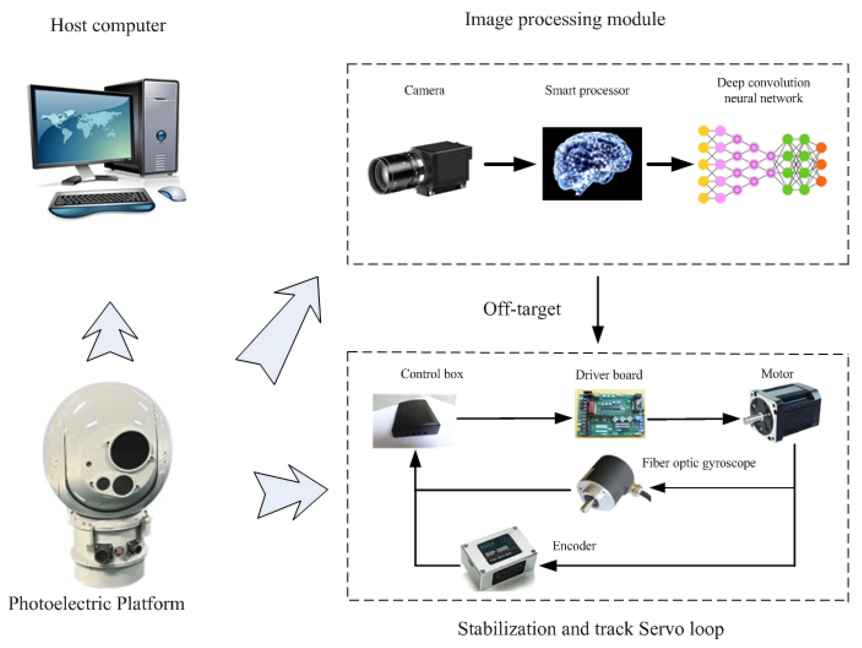
2.1. Architecture of the Photovoltaic Platform System
The photoelectric platform system mainly consists of a host computer, control box, driver board, motor, encoder, and fiber-optic gyroscope, as shown in Figure 1. As the key feedback angular velocity sensor, the output accuracy of the fiber-optic gyroscope seriously affects the pointing accuracy of the entire system platform [8,9].
2.2. Output Signal of Fiber Optic Gyroscope
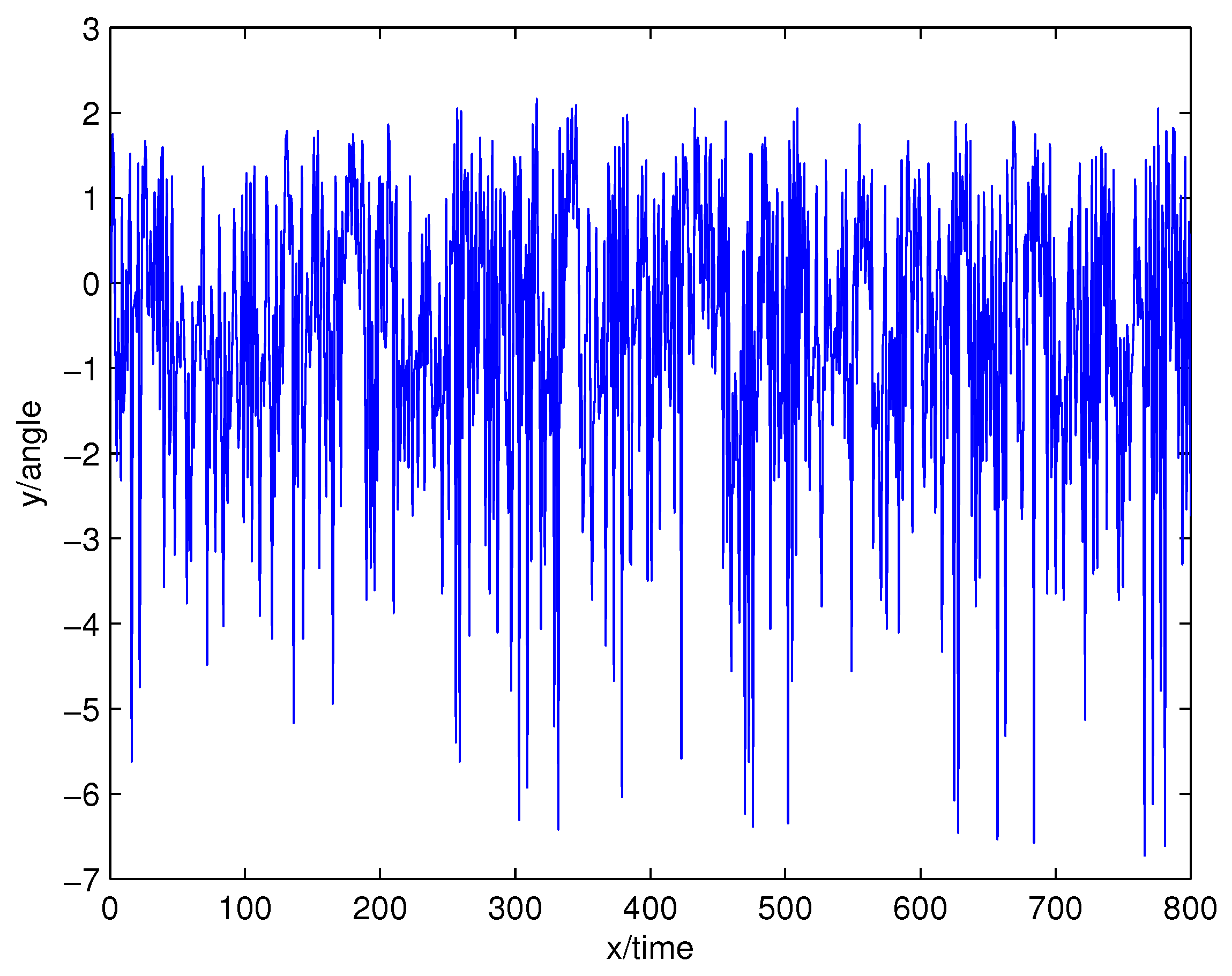
Through a long investigation, it was found that the fiber-optic gyroscope (FOG) has an output signal containing the angular velocity information of FOG, as well as the angular velocity information of the earth and various noises. Therefore, under the condition of a static pedestal, when the FOG measurement axis is perpendicular to the horizontal plane, the mathematical model of the gyro output is as follows:
In the above equation, is the angular rate of the earth’s rotation, L represents the local latitude, and is a constant zero offset (i.e., when the input angular rate is zero, the output constant of the gyroscope can be regarded as a constant in a short time). In addition, is the drift error, which has strong randomness and weak trend and periodicity. is white noise with a mean value of zero.
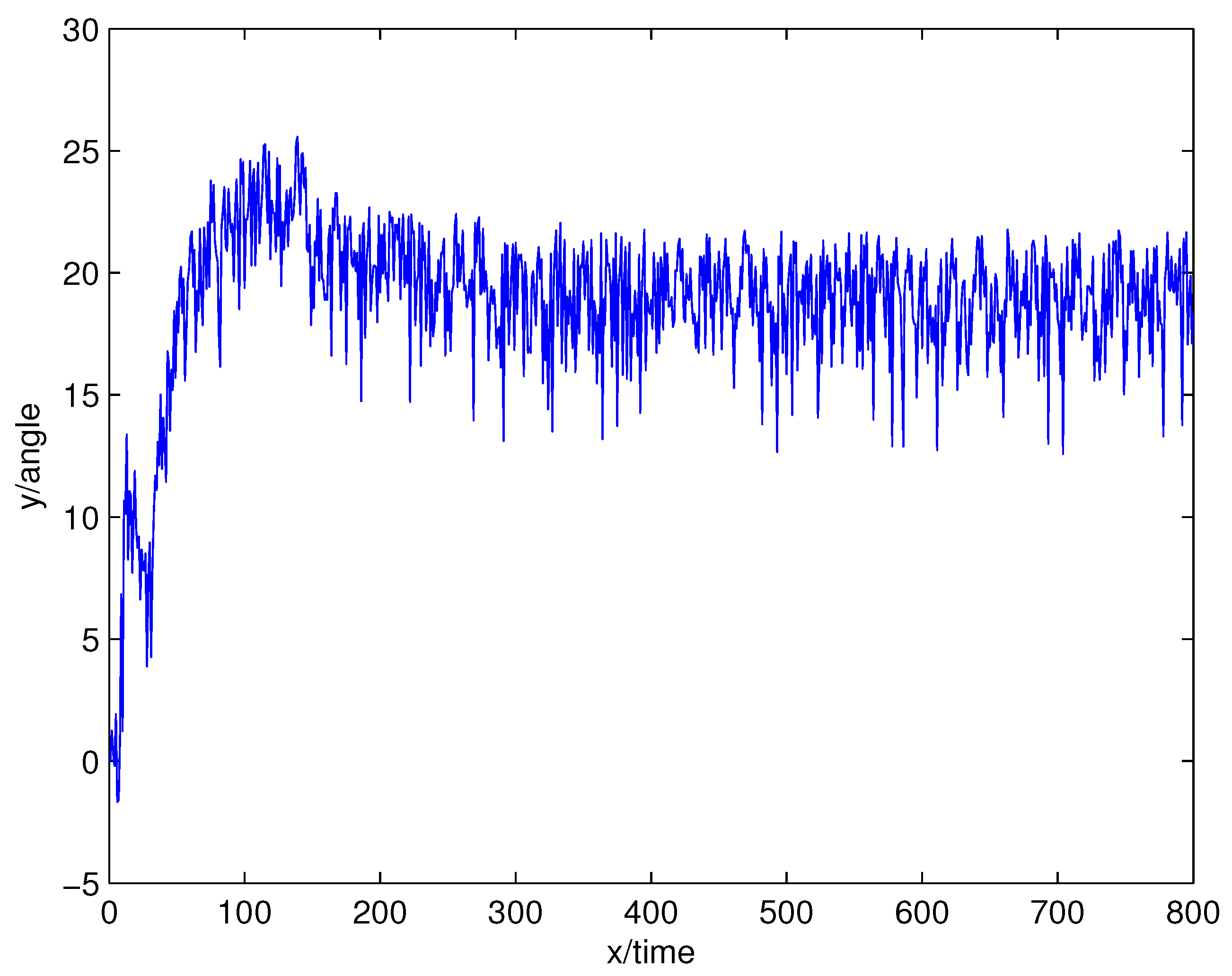
The original gyro output signal is shown in Figure 2.
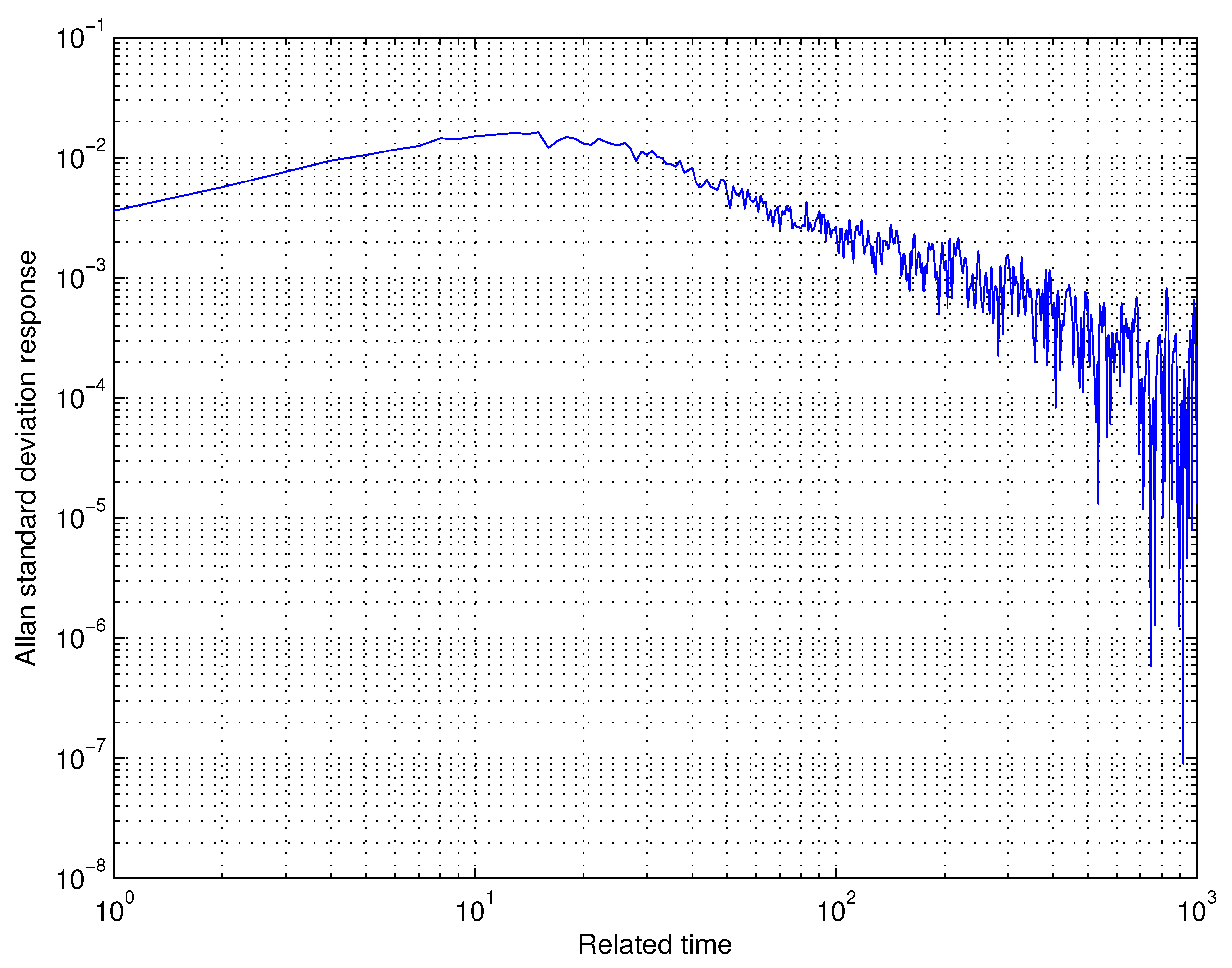
2.3. Allan Variance
Allan variance [10] is a famous method to characterize and identify various error sources in FOG, as well as their contribution to the statistical properties of the entire noise in detail. It is very easy to obtain types of error sources and the magnitude of each error source, by using the quantitative relationship between Allan variance and the power spectrum density (PSD). Here , is the output angular rate of FOG, acquired at a fixed sampling period . Then, sample the N initial samples again, with sampling time , where . Thus, the number of data packets is , and the average value of each time length is
At this time, the Allan variance on the time domain is defined as:
where is the difference between the average values of adjacent arrays, and is used to acquire the population mean. By selecting different array lengths (i.e., correlation time), the corresponding Allan variance and Allan standard deviation can be obtained.
In the frequency domain, the relationship of the bilateral power spectrum density between the Allan variance and the signal can be expressed by
where is PSD for random processes. The noise component in the FOG can be obtained quantitatively by means of Allan variance. These noise components mainly include angular random walk, zero offset stability, rate random walk, and speed ramp. It can be expressed as the following equation:
According to the relationship between the Allan variance and the power spectrum density function, the following equation can be obtained:
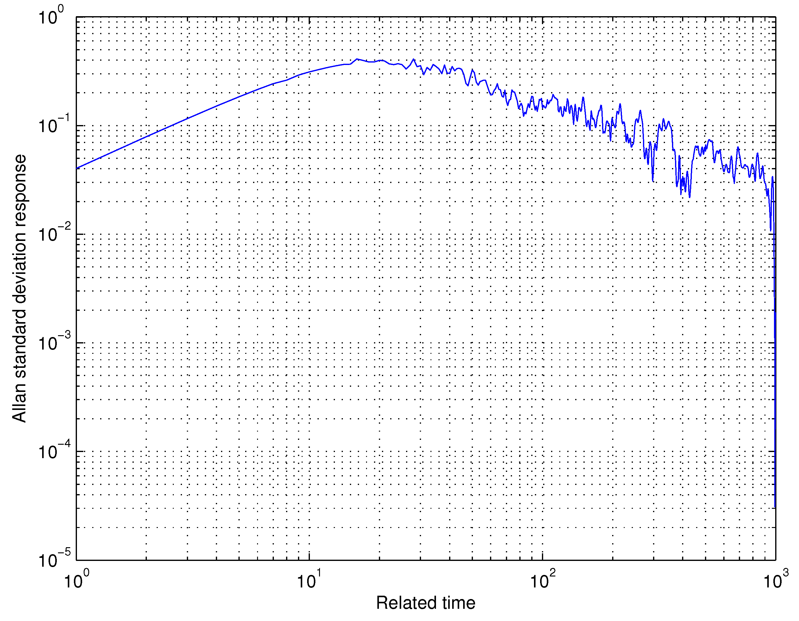
According to the gyro output data, the least-squares fitting method can be used to obtain the fitting coefficients, and the various noise systems can then be obtained by combining the equations. The Allan variance of the original gyro signal has been shown in Figure 3.
3. Related Knowledge
3.1. ARIMA Model
The ARIMA model is called the Auto Regressive Integrated Moving Average Model (ARIMA). It was proposed by Box and Jenkins in early 1970, to predict a time-series approach. ARIMA () is called a differential autoregressive moving average model, where AR is autoregressive, p is the autoregressive term, MA is the moving average, q is the moving average number, and d is the time series, which becomes a smooth difference number. The so-called ARIMA model refers to a model that converts a non-stationary time series into a stationary time series, and then returns the dependent variable (including the present and late value of the random error). Assuming that the data at time t is , it can be composed of weighted combinations of the p data before t time and corresponding errors, which is described in the following equation:
where to are the AR factor coefficients, and to are the MA factors. Here, the error sequence is assumed to be a white noise Gaussian distribution. Therefore, to establish the ARIMA model, it is necessary to determine the order of the model, evaluate the coefficients of the model, and predict the time series. Generally, the values of p and q are determined by correlation analysis, using an autocorrelation function and a partial correlation function. The parameters of the model are generally determined by the Box-Jenkins method, or the least-squares method [10,11,12]. In the paper, this is done by using an intelligent optimization algorithm.
3.2. Elman Model
An Elman neural network [13,14,15] is a kind of recursive network, which can approximate arbitrarily nonlinear functions with arbitrary precision. For the reason that a new layer is added to the hidden layer of the feed-forward network as a one-step delay operator to achieve memory ability, it has good approximation ability and dynamic characteristics. Additionally, it is well adaptive and self-organizing. Therefore, Elman networks have a wide range of applications, in areas such as function approximation, pattern recognition, and data compression.
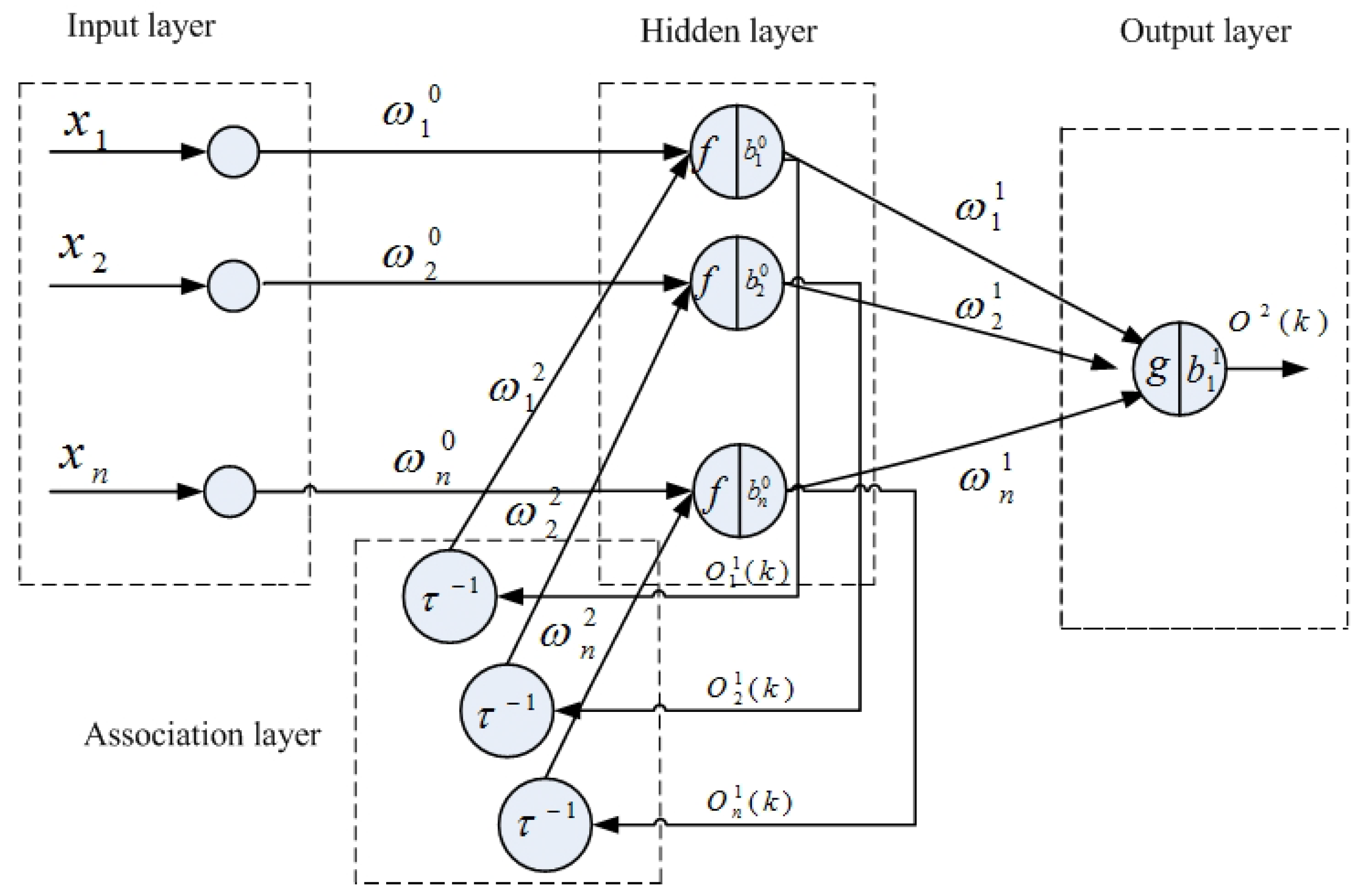
An Elman neural network is a feedback network, which can be regarded as a BP network with a local memory unit and local feedback connection. It consists of an input layer, several hidden layers, and an output layer. Each node in hidden layer has a corresponding associated layer node connection. In theory, a three-layer Elman network can approximate any nonlinear function with arbitrary precision. However, when there are too many neurons in the hidden layer, the convergence speed of the network is slow and the generalization ability of the network is poor. The generalization ability (also called comprehensive ability) refers to the capability that training with fewer samples enables the network to achieve the required accuracy in a given area, or using less training samples to give the network an appropriate output for untrained inputs. Therefore, a neural network without generalization capability has no practical value. According to the dynamic characteristics of inertial device error, this paper will use a four-layer Elman neural network; its structure is shown in Figure 4.
The output of the hidden layer is , that is, . is the output of the neuron, which can be expressed by . In addition, is the corresponding weight matrix. is the corresponding threshold.
As can be seen from Figure 4, the Elman network consists of an input layer, a hidden layer, an associative layer, and an output layer. The difference between an Elman neural network and a BP network lies in the existence of its associated layer nodes. Each hidden layer node has a corresponding associated layer node connection, and the weights of the links are adjustable. The output of the association layer node of an Elman neural network actually plays the role of storing the internal state of the network. The connection between the association layer and the middle layer is similar to the state feedback inside the system. The number of hidden layer nodes is the same as the number of nodes in the associated layer. Through the output of the associated layer node, the Elman network can store not only the current sequential input data, but also some of the past information in the sequential input data.
3.3. Lift Wavelet Filtering
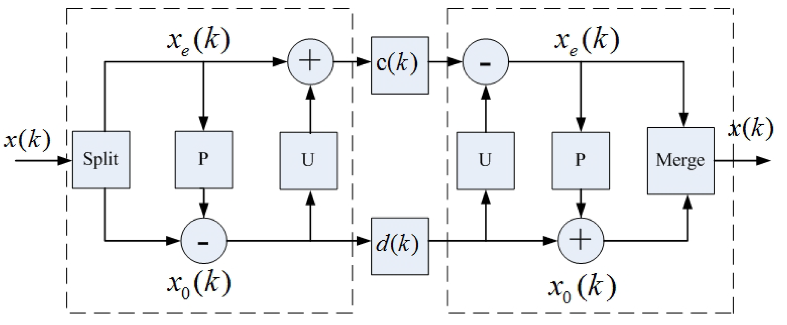
The lifting wavelet was proposed by Swenldens in 1996, and has been widely used in signal processing. The basic idea of the lifting algorithm is to gradually construct a wavelet with better properties through a basic wavelet. A canonical lifting algorithm has three steps; namely Split, Prediction, and Update, which is shown in Figure 5.
Split: The original sequence is divided into two disjoint subsets, each of which is half of the original sequence length. Typically, these two subsets are odd and even sequences, as follows:
Prediction: The wavelet coefficient is generated by using the prediction operator P. It can be expressed by the following formula:
Update: A better subset of data can be generated with the operator U, so that it can maintain the characteristics of the original data sequence . The update process is expressed, as follows:
At this point, one time of decomposition of the signal is completed with the wavelet. During reconstruction, the inverse update step is first operated to recover the even sequence, and then the inverse prediction step is operated to restore the odd sequence. Finally, the two sequences are placed, overlapping, to reconstruct the original signal.
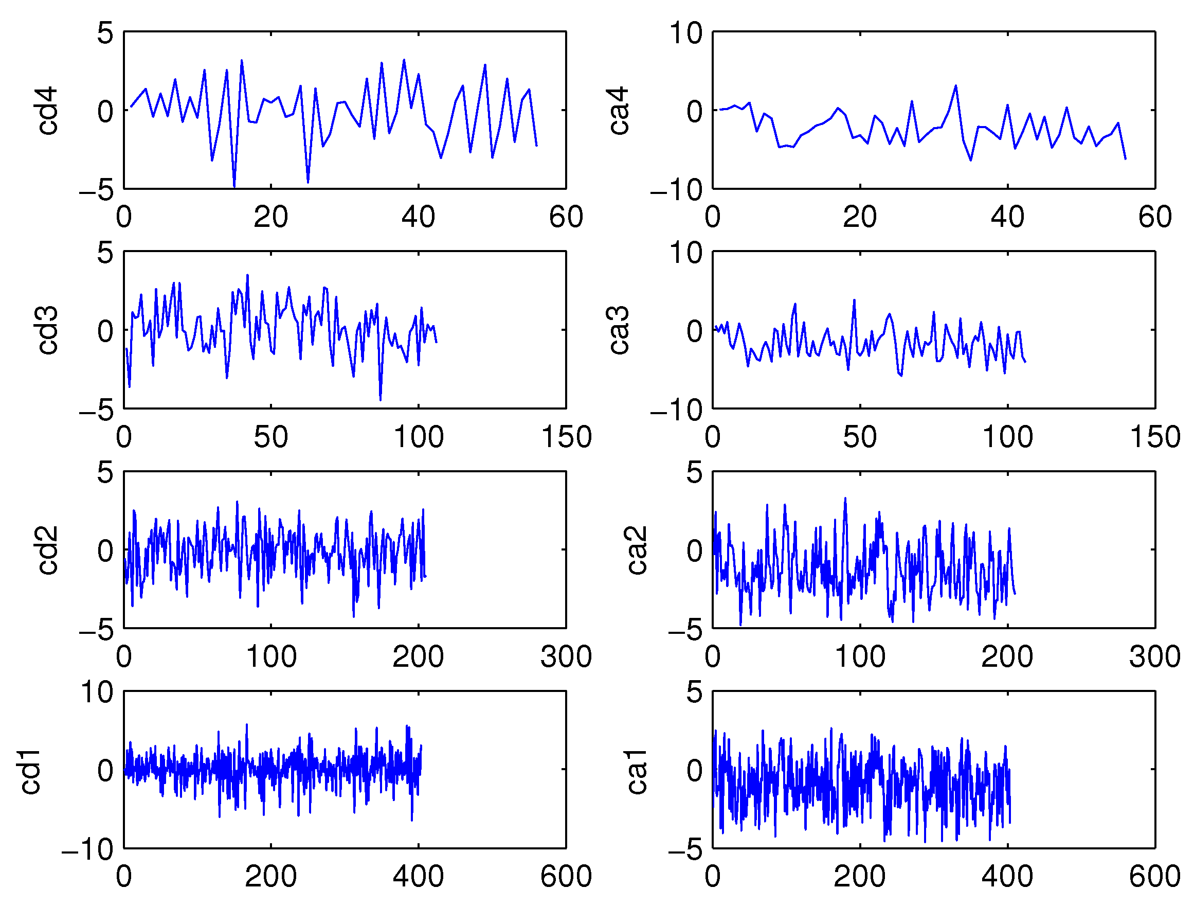
Due to the fact that gyro output contains white noise and drift error, it can be assumed that after a suitable p-time lifting wavelet decomposition, the drift error will be decomposed into and the white noise will be mainly decomposed into . Therefore, if the lifting wavelet reconstruction algorithm is used to reconstruct , the drift error can be obtained and the white noise can be obtained by reconstructing . Thus, the drift error and white noise are separated. This paper chooses the improved Haar wavelet as the wavelet base. When the decomposition order is 4, the decomposition and reconstruction results are shown in Figure 6 and Figure 7, respectively.
3.4. Differential Evolution
Differential Evolution (DE) [16,17] was proposed in 1997, by Rainer Storn and Kenneth Price, on the basis of evolutionary ideas (such as genetic algorithms). The essence is a multi-objective, continuous variable optimization algorithm for solving multi-dimensional optimal solutions in space. The source of differential evolution is the earlier-proposed genetic algorithm (GA) [18,19,20,21], which simulates crossover, mutation, and reproduction in genetics to design genetic operators.
The difference between the differential evolution algorithm and the genetic algorithm is that, in the differential evolution algorithm, the initial population is randomly generated and the fitness value of each individual in the population is selected as the selection criterion. The main process also includes three steps of mutation, intersection, and selection. The difference is that the genetic algorithm controls the parental hybridization according to the fitness value, and the probabilities generated by the mutation are selected. Therefore, the probability that the individuals with large adaptation values are selected in the maximization problem is correspondingly larger. In the differential evolution algorithm, the mutation vector is generated by the parent difference vector and intersects with the parent individual vector to generate a new individual vector, which is directly selected by the parent individual. Obviously, the approximation effect of the differential evolution algorithm is more significant than genetic algorithm [22,23].
For optimization problems, , such that , where D is the dimension of the solution space, and is the upper and lower bounds of , respectively. The flow of the algorithm is described, as follows:
Step 1: Population initialization
The initial swarm can be expressed by the following equation, where indicates population size and represents a random number distributed between (0, 1).
They can be generated randomly by the following equation:
where is the jth gene, representing chromosome 1 of the 0th generation.
Step 2: Mutation operation
Individual variation is derived through differential strategy:
where F is the scaling factor and indicates the ith individual in the g-generation population.
Step 3: Cross operation
Inter-individual cross-operation can be performed between the g-generation population .
otherwise,
where is its variant intermediates, is the crossover probability, and is a random integer within .
Step 4: Selection operation
uses greedy algorithms to select individuals which can enter the next generation of populations:
otherwise,
4. Hybrid ARIMA-Elman Model
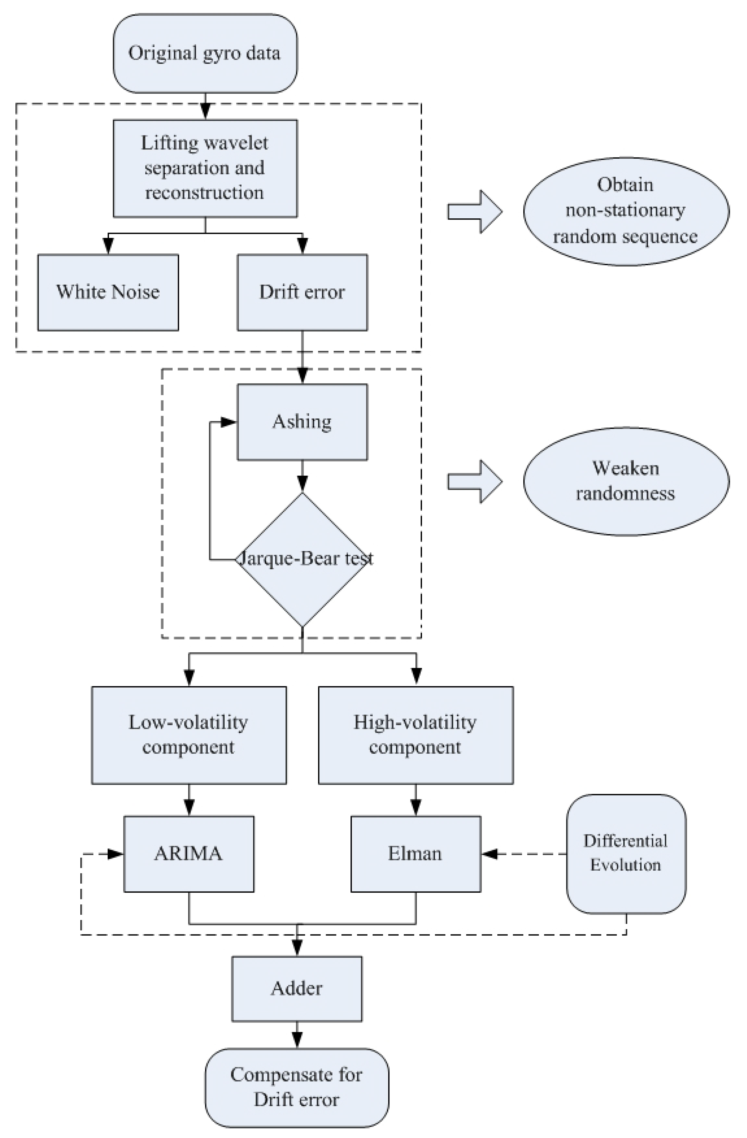
Firstly, lifting wavelet is used to preprocess the gyro data, to separate the high frequency white noise and low frequency drift component. Then, the low-frequency drift error belongs to the non-stationary random sequence, which can be further decomposed into linear components and nonlinear components. After that, the linear part is modeled using the ARIMA model, and the nonlinear part is modeled by the Elman neural network. Finally, the two partial prediction values are combined to compensate for drift error of the fiber-optic gyro.
4.1. Specific Steps
The specific steps are as follows:
Step 1: Acquire fiber-optic gyro error data.
Step 2: Decompose the original gyro error data into a white noise sequence and a drift error sequence, using the m-layer lifting wavelet transform. After the constant zero offset is compensated in the gyro static output, the signal output will only contain the drift error with low frequency and white noise with high frequency. Considering both performance of the algorithm and the actual requirements of the system, Harr wavelet and Daubechies wavelet basis functions are good choices. One reason is that these two wavelet basis functions have the characteristics of orthogonality and tight support. The other reason is that both the transform and inverse transform of these two wavelets can be explained succinctly by a linear orthogonal transform in matrix form, which is suitable for system programming. In this paper, in order to reduce the signal loss, a Daubechies wavelet with a second-order vanishing moment has been chosen. In theory, the higher the decomposition scale of the wavelet, the stronger the ability of characterizing the local characteristics of the signal will be. However, the amount of calculation is much greater at the same time. Therefore, we choose the db2 wavelet as a wavelet base, and 4 as the wavelet decomposition scale. For the reason that the drift error is a narrow-band signal with low frequency, and the white noise is a wide-band signal with high frequency, it can be determined that, after a suitable p-time lifting wavelet decomposition, the drift will be mainly decomposed into , and the white noise will be mainly decomposed into . Thus, if the reconstruction is performed separately for and using the lifting wavelet reconstruction algorithm, the drift error and white noise can be obtained, respectively. All of the above steps make it possible to separate the drift error from the white noise.
Step 3: Perform a graying strategy on the decomposed drift error; that is, perform one or more accumulation operations. Grey system theory is a new method to study small-sample problems, poor-information problems, and other uncertain problems. This method realizes the correct understanding and effective control of system behavior and evolution laws by generating and developing some known information and extracting valuable information. The ashing operation generates the new data through accumulating the original data, which can weaken the randomness of the original data and enhance its regularity to a certain extent. Therefore, it makes it simple to get the change law of the data. Then, a standard Jarque-Bear test is used to judge the grayed output data. In general, to diagnose whether a given sequence is normally distributed or not, the Jarque-Bear normality test can be performed, as illustrated in Equation (18). If the value is close to 3, the sequence is Gaussian distributed and linear, which can be approximated by an ARIMA model. Otherwise, it is nonlinear and is suitable to be approximated by an Elman neural network. In the test, whether the kurtosis of the data is 3 or not is based on the equation:
where x is the random sequence and E is the expectation operation.
Step 4: The values close to 3 (through test equation Jarque-Bear) are modeled using the ARIMA model, and the remainder is approximated using the Elman neural network. Meanwhile, use the differential evolution algorithm to determine the ARIMA model parameters and neural network weight values. It is well known that the parameters of the ARIMA and Elman neural network models are difficult to determine. For example, the values of AR factor coefficients (i.e., ) and values of MA factors (i.e., ) should be determined. As Section 3.2 depicted, in the Elman neural network model, values of the weight matrix , , and threshold matrix , also need to be determined. In fact, the problem can be seen as a combination optimization problem. In detail, it is to seek the best combination of model parameters which make the difference between the predicted outputs and the actual values as small as possible for each sample. Therefore, the intelligent optimization algorithm (i.e., DE algorithm) is first used in handling the problem. Here, as Section 3.4 illustrated, population initialization is initially operated. For both of the parameter optimizations of the ARIMA and Elman neural network models, the scaling factor F is set to 0.6 and the crossover probability is set to 0.8. Finally, through mutation operation, cross operation, and selection operation, the optimization values of parameters can be obtained.
Step 5: Combine the values of the two predictions.
The flow chart of the proposed hybrid ARIMA-Elman model is described in detail, as follows in Figure 8:
4.2. The Final Compensation Results
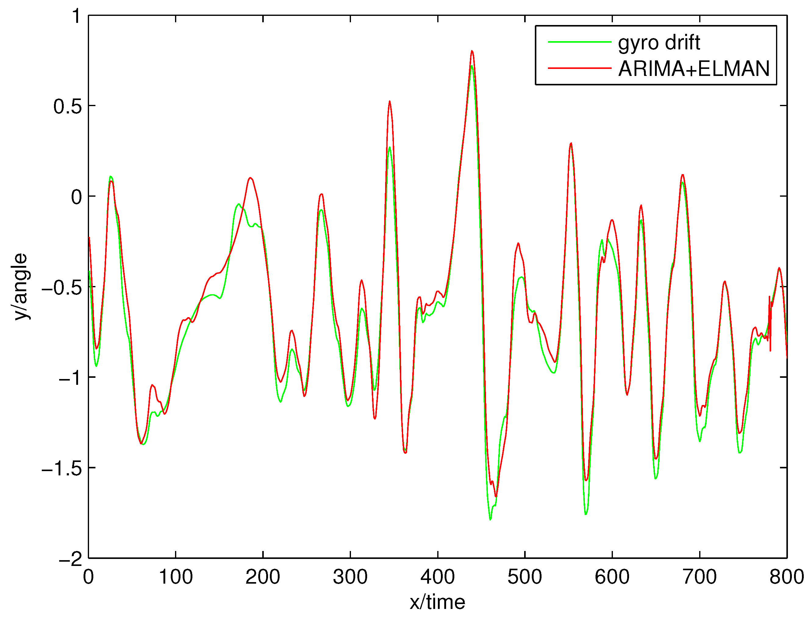
Through four-layer lift-wavelet decomposition and reconstruction, the drift component contained in the original gyro signal is obtained. Through steps 1 to 5 depicted in Section 4.1, the drift error can be approximated finally, as shown in Figure 9. Figure 10 shows the Allan variance after compensation, based on the hybrid ARIMA-Elman method. From Figure 9, it can be easily seen that the reconstructed drift error can be approximated by the proposed ARIMA-Elman model with high precision. The red and green lines are basically coincident. From Figure 10, we can conclude that the Allan variance value is much smaller after compensation, when compared with Figure 3. This phenomenon illustrates that the high frequency white noise and the non-stationarily distributed drift error have been compensated for fully. In addition, in order to explain the superiority of the proposed hybrid method, the compensation results with different methods have been listed in Table 1. From the table, it is very easy to see that all the coefficients of the main types of noise (quantization noise, angle random walk noise, zero offset instability noise, rate random walk noise, and rate ramp noise) have reduced, compared with the original signal. However, neither the single ARIMA model, nor the single Elman model, obtain better results than the hybrid ARIMA-Elman model. For example, in the original signal, the coefficient of quantization noise is −105.3339, and with the single ARIMA method, the value changes to −12.0008. With the single Elman method, the value changes to −4.8718. Meanwhile, with the ARIMA-Elman method, it changes to −0.2821. Especially for the rate ramp noise, the noise coefficient changes to zero after compensation using the proposed hybrid method. Furthermore, all of the other coefficient values have reduced sharply as well. All of these prove the effectiveness and superiority of the proposed method.
The change of error coefficients, before and after compensation, with different methods are shown in Table 1.
From the above comparison results, it can be easily seen that all of the error coefficients in the hybrid model are the smallest. After compensation, the coefficient of the rate random walk noise is zero. All of these illustrate that the proposed hybrid method can achieve satisfactory compensation results.
4.3. Generalization Test
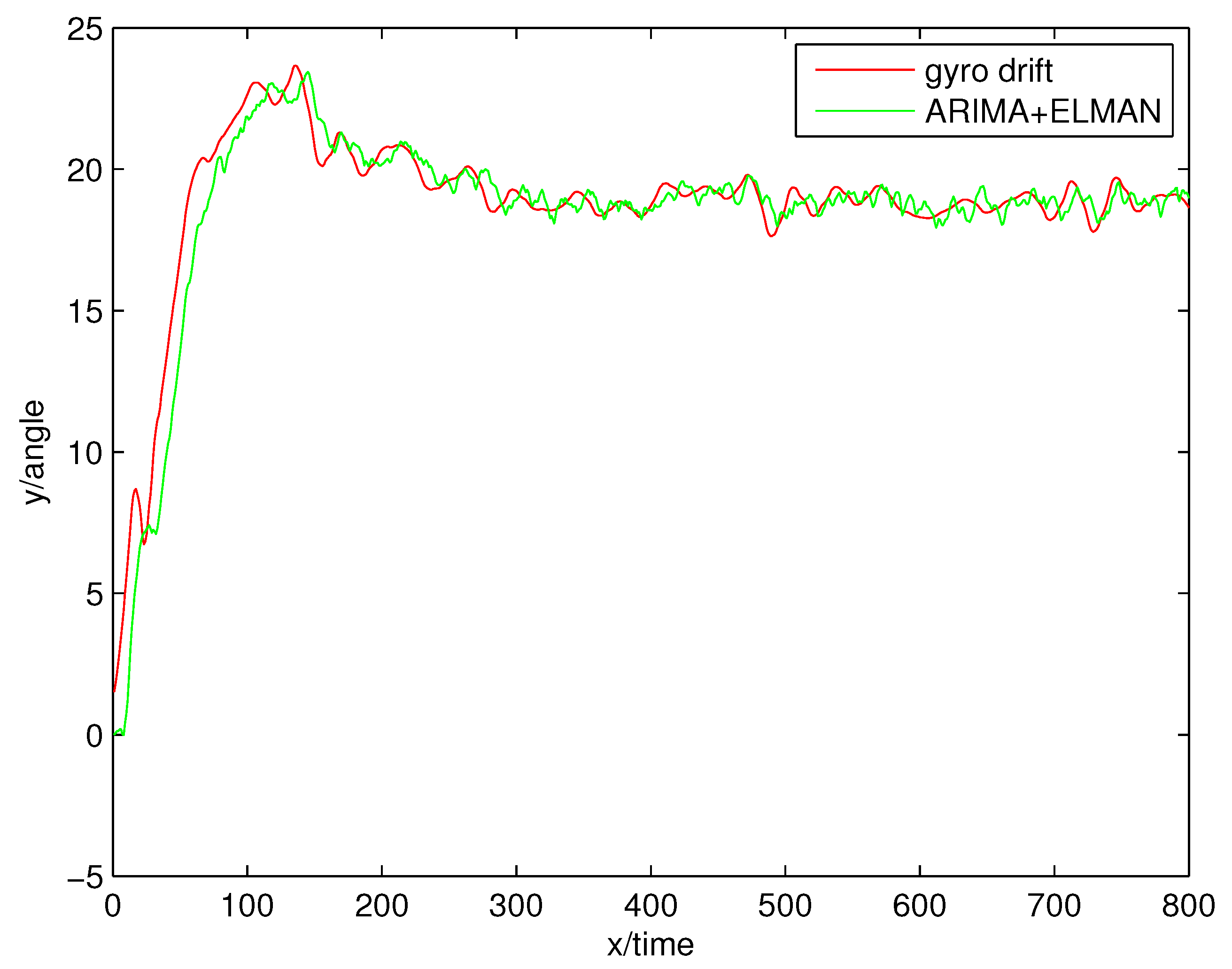
In order to test the generalization ability of the method, another type of gyro data has been collected. The gyro signal is shown in Figure 11. According to the above-mentioned method, similar steps have been carried out concerning the new gyro error. The results, after compensation, are shown in Figure 12, and the relative comparison is provided in Table 2. From Figure 12, we can see that the red and green lines are basically coincident.
The change of error coefficients, before and after compensation, with different methods are shown in Table 2. In the table, all of the coefficient changes of the main types of noise contained in the gyro signal (quantization noise, angle random walk noise, zero offset instability noise, rate random walk noise, and rate ramp noise) have been listed. We can see that all of the item values have reduced after compensation with different methods. Among the three methods (single ARIMA model, single Elman model, and hybrid ARIMA-Elman model), the change with the hybrid model is the most significant one. The former two algorithms achieve similar results, which are close to the original values. For example, for the quantization noise, the coefficient of the original signal is 28.4648. After compensation, the value changes to be 22.0082, 20.1009, and −0.1692, respectively.
From Figure 12 and Table 2, it can be easily seen that, compared with a single linear or nonlinear approximation model, the Allan variance coefficients are the smallest when using the hybrid model. Therefore, it can be concluded that the hybrid method has good generalization ability and can be easily applied in similar fields, which is very important particularly in engineering fields.
5. Conclusions
Affected by external vibration, temperature change, and other factors, fiber-optic gyro in a photoelectric system usually causes complex errors, which can seriously reduce servo performance and even cause divergence of the whole system. Therefore, gyro error compensation techniques have attracted the attention of many experts for a long time. However, according to the current literature, due to the non-stationary randomness, the typically-used either single linear approximation model or single nonlinear neural network approximation model did not work well. In this paper, based on the lift-wavelet separation and reconstruction technique, the relative low-frequency drift error component was first obtained. Then, in order to weaken the randomness of the data sequence, an ashing technique was operated and drift error separated into low-volatility and high-volatility components. After that, the ARIMA model and recurrent Elman model was applied, to compensate for each component independently. As the hybrid ARIMA-Elman model combines the advantages of both of the two models, it can fully collect complex nonlinear characteristics hidden in non-stationary drift error data and approximate them better, theoretically. Furthermore, taking into consideration that the commonly used least-squares method, genetic optimization algorithms, and so on, easily fall into local extreme values and model parameters are difficult to determine, in this paper an intelligent difference algorithm was proposed to identify parameters of the hybrid model. The algorithm had few parameters to adjust, which saved much time during the training stage. The gyro data was actually collected and processed, and, based on the famous Allan variance, the data (before and after compensation) was compared and analyzed, respectively. Experimental results showed that the proposed method in the study can filter out the non-stationary noise in the gyro quickly and effectively. Furthermore, to test the generalization ability of the method, another set of data was collected and compensated using the proposed hybrid model and the above-mentioned data process technique. The experimental results meanwhile showed that the proposed method in this paper has good generalization capability, and can meet actual engineering needs satisfactorily.
Author Contributions
X.X. and Q.H. conceived and designed the experiments; C.W. and Z.F. analyzed the data; C.W. contributed analysis tools; X.X. wrote the paper.
Funding
The paper was supported by the National Science Foundation of China (grant no. 61705052) and the Fundamental Research Funds for the Central Universities (grant no. HIT.NSRIF.201630).
Conflicts of Interest
The authors declare no conflict of interest.
References
- Sander, G.A.; Szafrenie, B.; Liu, R.Y.; Laskoskie, C.L.; Strandjord, L.K.; Weed, G. Fiber Optic Gyros for Space, Marine, and Aviation Application. Proc. SPIE 1996, 2837, 61–71. [Google Scholar]
- Ulrich, R. Fiber-optic Rotation Sensing with Low Drift. Opt. Lett. 1980, 5, 173–175. [Google Scholar] [CrossRef]
- Fang, S.N.; Zhang, C.X.; Jin, J. Phenomena of Optic-bound Effect on Fiber Optic Gyro. Chin. Phys. 2007, 16, 735–739. [Google Scholar] [CrossRef]
- Allan, D.W. Statistics of Atomic Frequency Standards. Proc. IEEE 1966, 54, 221–230. [Google Scholar] [CrossRef]
- Blin, S.; Kim, H.K.; Digonnet, M.; Kino, G.S. Reduced thermal sensitivity of a fiber-optic gyroscope using an air-core photonic-band gap fiber. J. Light Wave Technol. 2007, 25, 861–865. [Google Scholar] [CrossRef]
- Long, Y.W.; Hui, T.Y.; Yu, X.W.; Zhang, L. Application of artificial neural network and genetic algorithm in modeling of fiber optic gyroscope temperature drift. Artif. Intell. 2006, 22, 273–275. [Google Scholar]
- Zhu, R.; Zhang, Y.H.; Bao, Q.L. Identification of temperature drift for FOG using RBF neural networks. J. Shang Hai Jiao Tong Univ. 2000, 32, 221–225. [Google Scholar]
- Kojima, H.; Hiraiwa, K.; Yoshimura, Y. Experimental study on line-of-sight (LOS) attitude control using control moment gyros under micro-gravity environment. Acta Astronaut. 2018, 143, 118–125. [Google Scholar] [CrossRef]
- Leeghim, H.; Kim, D. Adaptive neural control of spacecraft using control moment gyros. Adv. Space Res. 2015, 55, 1382–1393. [Google Scholar] [CrossRef]
- Lv, P.; Liu, J.Y.; Lai, J.Z.; Huang, K. Allan variance method for gyro noise analysis using weighted least square algorithm. Optik 2015, 126, 2529–2534. [Google Scholar] [CrossRef]
- Zhou, S.C.; Li, X.L.; Ga, Y.P.; Chen, H.P. A multi-objective differential evolution algorithm for parallel batch processing machine scheduling considering electricity consumption cost. Comput. Oper. Res. 2018, 96, 55–68. [Google Scholar] [CrossRef]
- Fontanellaa, R.; Accardoa, D.; Morielloa, R.S.; Angrisani, L.; Simonec, D.D. MEMS gyros temperature calibration through artificial neural networks. Sens. Actuators A Phys. 2018, 279, 553–565. [Google Scholar] [CrossRef]
- Achanta, S.; Gangashetty, S. Deep Elman recurrent neural networks for statistical parametric speech synthesis. Speech Commun. 2017, 93, 31–42. [Google Scholar] [CrossRef]
- Ruiz, L.G.; Rueda, R.; Cuellar, M.P.; Pegalajar, M.C. Energy consumption forecasting based on Elman neural networks with evolutive optimization. Expert Syst. Appl. 2018, 92, 380–389. [Google Scholar] [CrossRef]
- Hsu, C.F. Adaptive backstepping Elman-based neural control for unknown nonlinear systems. Neurocomputing 2018, 130, 264–278. [Google Scholar] [CrossRef]
- Subudhi, B.; Jena, D. A differential evolution based neural network approach to nonlinear system identification. Appl. Soft Comput. 2011, 11, 861–871. [Google Scholar] [CrossRef]
- Tang, H.; Xue, S.; Fan, C. Differential evolution strategy for structural system identification. Comput. Aided Civ. Infrastruct. Eng. 2011, 26, 92–110. [Google Scholar] [CrossRef]
- Karaboga, D.; Okdem, S. A simple and global optimization algorithm for engineering problems: differential evolution algorithm. Turk. J. Electr. Eng. Comput. Sci. 2004, 12, 53–60. [Google Scholar]
- Raman, M.R.; Somu, N.; Kirthivasan, K.; Liscano, R.; Sriram, V.S. An efficient intrusion detection system based on hyper graph - Genetic algorithm for parameter optimization and feature selection in support vector machine. Knowl.-Based Syst. 2017, 134, 1–12. [Google Scholar] [CrossRef]
- Baek, S.H.; Park, D.H. Hybrid kernel density estimation for discriminant analysis with information complexity and genetic algorithm. Knowl.-Based Syst. 2016, 99, 79–91. [Google Scholar] [CrossRef]
- Chettah, A.K.; Talbi, H. A Compound Sinusoidal Differential Evolution algorithm for continuous optimization. Swarm and Evolutionary Computation. Swarm Evol. Comput. 2018. [Google Scholar] [CrossRef]
- Qin, F.Q.; Feng, Y.X.; Lian, Z.Y. Auto-selection mechanism of differential evolution algorithm variants and its application. Eur. J. Oper. Res. 2018, 270, 636–653. [Google Scholar]
- Zorlu, H. Optimization of weighted myriad filters with differential evolution algorithm. AEU-Int. J. Electron. Commun. 2017, 77, 1–9. [Google Scholar] [CrossRef]
Figure 1.
Photoelectric platform system.

Figure 2.
The original gyro signal.

Figure 3.
ALLAN variance of the original gyro signal.

Figure 4.
Structure of an Elman neural network.

Figure 5.
Structure of the lifting algorithm.

Figure 6.
Decomposition results of a 4-layer wavelet.

Figure 7.
Reconstruction of the drift error.

Figure 8.
Flow chart of the hybrid ARIMA-Elman model.

Figure 9.
Approximation results based on the ARIMA-Elman method.

Figure 10.
Allan variance after compensation.

Figure 11.
The original gyro data.

Figure 12.
Compensation results based on the ARIMA-Elman method.


Table 1.
Comparison results of coefficients before and after compensation. Here, QN indicates Quantization Noise, ARW indicates Angle Random Walk, ZOI indicates Zero Offset Instability, RRW indicates Rate Random Walk, and RR indicates Rate Ramp.
Table 1.
Comparison results of coefficients before and after compensation. Here, QN indicates Quantization Noise, ARW indicates Angle Random Walk, ZOI indicates Zero Offset Instability, RRW indicates Rate Random Walk, and RR indicates Rate Ramp.
| Noise Type | QN | ARW | ZOI | RRW | RR |
|---|---|---|---|---|---|
| Original signal | −105.3339 | 151.0151 | −3.9396 | 0.0399 | 0.0028 |
| ARIMA | −12.0008 | 20.8510 | −0.2162 | −0.0102 | 0.0017 |
| ELMAN | −4.8718 | 2.8510 | −0.0162 | −0.0079 | 0.0010 |
| ARIMA + ELMAN | −0.2821 | 0.2115 | −0.0273 | 0.0015 | −0.0000 |
Table 2.
Comparison results of coefficients before and after compensation. Here, QN indicates Quantization Noise, ARW indicates Angle Random Walk, ZOI indicates Zero Offset Instability, RRW indicates Rate Random Walk, and RR indicates Rate Ramp.
Table 2.
Comparison results of coefficients before and after compensation. Here, QN indicates Quantization Noise, ARW indicates Angle Random Walk, ZOI indicates Zero Offset Instability, RRW indicates Rate Random Walk, and RR indicates Rate Ramp.
| Noise Type | QN | ARW | ZOI | RRW | RR |
|---|---|---|---|---|---|
| Original signal | 28.4648 | −23.8923 | 6.7926 | −0.4592 | 0.0089 |
| ARIMA | 22.0082 | −21.9880 | 6.5200 | −0.4321 | 0.0086 |
| ELMAN | 20.1009 | −21.1266 | 6.4341 | −0.4294 | 0.0081 |
| ARIMA + ELMAN | −0.1692 | 0.0382 | 0.0323 | −0.0042 | 0.0001 |
© 2019 by the authors. Licensee MDPI, Basel, Switzerland. This article is an open access article distributed under the terms and conditions of the Creative Commons Attribution (CC BY) license (http://creativecommons.org/licenses/by/4.0/).
Share and Cite
MDPI and ACS Style
Xu, X.; Wu, C.; Hou, Q.; Fan, Z. Gyro Error Compensation in Optoelectronic Platform Based on a Hybrid ARIMA-Elman Model. Algorithms 2019, 12, 22. https://0-doi-org.brum.beds.ac.uk/10.3390/a12010022
AMA Style
Xu X, Wu C, Hou Q, Fan Z. Gyro Error Compensation in Optoelectronic Platform Based on a Hybrid ARIMA-Elman Model. Algorithms. 2019; 12(1):22. https://0-doi-org.brum.beds.ac.uk/10.3390/a12010022
Chicago/Turabian StyleXu, Xingkui, Chunfeng Wu, Qingyu Hou, and Zhigang Fan. 2019. "Gyro Error Compensation in Optoelectronic Platform Based on a Hybrid ARIMA-Elman Model" Algorithms 12, no. 1: 22. https://0-doi-org.brum.beds.ac.uk/10.3390/a12010022
Note that from the first issue of 2016, this journal uses article numbers instead of page numbers. See further details here.