YeastNet: Deep-Learning-Enabled Accurate Segmentation of Budding Yeast Cells in Bright-Field Microscopy

Abstract

Accurate and efficient segmentation of live-cell images is critical in maximizing data extraction and knowledge generation from high-throughput biology experiments. Despite recent development of deep-learning tools for biomedical imaging applications, great demand for automated segmentation tools for high-resolution live-cell microscopy images remains in order to accelerate the analysis. YeastNet dramatically improves the performance of the non-trainable classic algorithm, and performs considerably better than the current state-of-the-art yeast-cell segmentation tools. We have designed and trained a U-Net convolutional network (named YeastNet) to conduct semantic segmentation on bright-field microscopy images and generate segmentation masks for cell labeling and tracking. YeastNet enables accurate automatic segmentation and tracking of yeast cells in biomedical applications. YeastNet is freely provided with model weights as a Python package on GitHub.

1. Introduction

S. cerevisiae, hereafter referred to as yeast, is a eukaryotic model organism used to study synthetic gene network development and analysis, as well as other biological processes. Bright-field and fluorescence microscopy are common approaches to investigate yeast behavior. The quantitative analysis of time-lapse fluorescence microscopy images is a powerful tool for large-scale and single-cell analysis of dynamic and noisy cellular processes, such as gene expression [1,2,3]. In an experimental design wherein yeast cells are expressing a fluorescent marker of interest, quantitative analysis involves the quantification of fluorescence intensity of pixels corresponding to cell regions in a microscopy image of those cells. Therefore, quantitative analysis requires accurate identification of cell regions, known as segmentation, as well as tracking of these cell regions between images, in the case of time-lapse microscopy.

In recent years, automated light microscopes have been paired with commercial or lab-constructed microfluidics devices to conduct time-lapse analysis of cell cultures in long-term perfusion conditions. Microfluidics-enabled time-lapse fluorescence microscopy allows the study of dynamic cellular processes in a single-cell manner. Automated image capturing of multiple fields of view at high imaging frequencies increases the number of tracked cells and enhances the resolution of the data. However, it also greatly increases the number of images that need to be analyzed from hundreds to tens of thousands. Thus, automated solutions for the problem of cell segmentation are necessary to avoid very time-consuming and error prone manual segmentation.

One way to address the segmentation problem has been the use of fluorescent markers expressed in the cytosol to label cells in fluorescence images. For example, cells with constitutively expressed green fluorescent protein (GFP) are easily separable from a background when imaged with a green light filter. Cell segmentation in fluorescence images is easier than that in corresponding bright-field images; however, the number of different fluorescent proteins (FPs) that can be used in an experiment is limited [4]. Due to overlapping excitation and emission spectra of many FPs, as well as the effects of Förster resonance energy transfer (FRET), using multiple different FPs requires careful selection. Moreover, additional fluorescent imaging increases the risk of phototoxicity and photobleaching. Although use of fluorescent markers can be beneficial in some cases, cell segmentation from bright-field images is required in most cases. Therefore, the ideal algorithm for cell segmentation should work automatically from a bright-field image input.

Several features of yeast cells in bright-field images have been used for segmentation by non-trainable (manually parameterized) algorithms or manual analysis. A cell’s outline is generally its most distinguishable 2D structure in a bright-field image due to the distinct brightness of the outline relative to the cell interior and background. In slightly out-of-focus bright-field images, this outline is thicker and easier to identify using thresholding techniques [5]. However, several characteristics of yeast cells prevent accurate segmentation with these traditional algorithms, particularly in the case of time-lapse microscopy wherein distinguishable features of cell outlines usually change over time. Yeast cells divide quickly, forming colonies of tightly packed cells within hours. In such dense colonies neighboring cells converge or overlap, making detection of individual outlines very difficult. Additionally, cell outlines may change in brightness and thickness due to focus drift of the microscope over time.

The history of image segmentation algorithms is long and varied. The simplest method of automated image segmentation is thresholding, in which a brightness threshold is manually selected and every pixel in an image is classified as foreground if it is higher or background if it is lower. This method was known to be poor as early as the 60s [6] and newer and better performing algorithms have been developed since. One of the seminal developments in this field is Otsu’s method [7] which improved upon previous thresholding algorithms by developing a non-parametric and unsupervised method for selecting the threshold. In Otsu’s method, the threshold is chosen by minimizing the intra-class variance of the foreground and background pixels. Although Otsu’s method was a great development, it suffers from several limitations including noise and small object size. A modification to Otsu’s method to address issues with noisy images called the two-dimensional Otsu’s method was published in 1991 [8]. It improved performance on noisy images by comparing pixel intensity variance within a pixel’s neighborhood rather than globally.

A difficulty with image segmentation comes from brightness gradients across images. A single threshold is not enough to deal with this problem. Adaptive thresholding, where a new threshold is calculated for every pixel is therefore necessary for this task. An algorithm developed in 2007 [9], uses the integral image to calculate the average pixel intensity around a pixel and if the intensity is a certain threshold below the average, it is set to black, otherwise it is set to white. The advantage of this algorithm is it performs well on images with spatial variation of illumination, and it is very fast to compute.

Interactive segmentation algorithms are also a popular set of methods for image segmentation. These include tools such as the Lasso tool in Adobe Photoshop, as well as Lazy Snapping [10] and Grabcut [11]. Lazy Snapping and Grabcut are accurate tools that involved user input to help locate the general area of the boundary. In the case of Grabcut, a bounding box was drawn by the user around the object of interest, and iterative graph cuts employed by the algorithm would segment the object inside the bounding box. Meanwhile for Lazy Snapping, lines would be drawn by the user to indicate the general area of the foreground and background and graph cuts would place a deformable edge around the object, allowing the user to correct any errors. A similar user interface is involved in [12], which requires the user to scribble different regions of interest in an image. The advantage of these tools was mainly ease of use, but the interactive nature did not make them useful in high-throughput settings such as biomedical imaging.

A class of segmentation algorithms using active contours were developed in the 80s, 90s and 2000s. Kass et al. introduced the Snakes active contour algorithm in 1988 [13]. The Snakes algorithm uses energy minimization to fit deformable splines to the contours of objects in images. They were able to solve problems that had up to that point eluded accurate segmentation, especially in images with a lot of noise. The Snakes algorithm, however, was not completely automatic and required user input to move splines out of local minima. Extensions to this work involved improvements to the types of active contours that were used, the energy definition and the energy minimization algorithms used [14,15].

The watershed algorithm, developed by [16] is a segmentation algorithm with a very intuitive explanation. It looks at an image as a topographical relief map. The image is ‘flooded’ at the local minima in the image and the places where different sources of water touch are used as segmentation boundaries. Meyer improved the algorithm by introducing markers as sources for flooding, avoiding the issues with having flooding from all regional minima [17]. By indicating the sources of flooding with early approximations of the objects of interest, watershed segmentation performs very well and is often included in segmentation and tracking pipelines even now [18,19].

Many algorithms have been presented for the cell segmentation problem over the past decade. Unsupervised algorithms which use computer vision processes such as the aforementioned watershed algorithm [18], and active contour fitting [20,21] are popular solutions. An updated version the 2013 Doncic algorithm was reported in 2019 [19] with improved watershed marker selection, a step that used to be interactive. It also takes advantage of the fact that all cells are present in the final image in a time-series, by starting from the final image and working backwards they simplify the problem of detecting and tracking new cells. Recently, hybrid algorithms using pipelines of multiple processes with manual user supervision have become more common. One of these methods called CellStar uses thresholding and active contour fitting, in addition to user-enabled automated parameter fitting. CellStar shows the highest segmentation accuracy for a variety of data sets [21].

Most recent computer vision tools have leveraged the power of deep learning. This became possible with the development of the convolutional neural net (CNN) which uses convolutional layers over fully connected layers, the building blocks of the original neural networks. The multi-perception, the original deep-learning network architecture was not suited for use on multi-dimensional data such as images so the CNN was developed to handle the increased computational power required to use deep learning with images. The critical change introduced with the CNN is the convolutional layer which reduces the connections between neurons to only a neighborhood of pixels rather than the whole image, as well as weight sharing. The convolutional layer, paired with the pooling layer, which reduces the resolution of convolutional feature maps, combine to allow for deep convolutional networks to learn features at multiple scales. These feature maps are then fed into a fully connected layer to make a class prediction. An example of a simple 2-layer convolutional network is shown in Figure 1. A more in-depth description of CNNs can be found in [22,23].

CNNs have been adopted across nearly every discipline for their many advantages over previous algorithms. Model inference is fully automated and CNNs can be trained to be exceptionally accurate. In addition, since images often share similar features, common pre-trained models can be reused in different domains in a process called transfer learning. CNNs suffer from several disadvantages which involve the requirement of a large number of labeled images for training as well as lengthy training times. CNNs are also computationally intensive to train and run, though the ability to train CNNs on Graphics Processing Units (GPUs) can speed this up greatly.

In recent years, CNNs have been extended to the task of semantic segmentation and led to new possibilities in the field of biomedical imaging. Semantic segmentation is the process of segmenting an image into multiple classes by classifying each pixel in an image. The fully convolutional network for semantic segmentation [24] is the seminal architecture that introduced the ability to train a network to output pixel-wise class predictions for an input image. The fully connected layers usually found at the end of CNNs and used to classify images were replaced with learned convolutional up-sampling layers. By using up-sampling layers, the down-sampling of the encoder layers is reversed, and the output of the network maintains the resolution of the input image. In order to improve the up-sampling layer, feature maps obtained at earlier stages of the network are appended to the final layer via skip connections. It has been discovered that the increase in the number of connections leads to higher accuracy of the network [24].

In 2015, the U-Net architecture [25] improved classification accuracy achieved with the fully convolutional semantic segmentation networks introduced by Long et al. [24]. The U-Net was developed for the task of pixel-wise cell segmentation of mammalian cells. By implementing skip connections for every layer in the down-sampling half of the network, each up-sampling layer consisted of twice the data. The U-Net demonstrated that it was not necessary to have very large annotated datasets to achieve high accuracy in segmentation tasks using deep learning.

Deep-learning approaches for cell segmentation have been developed for various cell types and imaging methodologies. DeepCell [26], developed in 2016, is a deep-learning model based on CNNs developed to segment bacterial and mammalian cells, but it has not been used for yeast cells. In 2017, a model trained to analyze yeast cells was published [27] based on the SegNet [28] architecture. The SegNet architecture is similar to the U-Net in that it follows a fully convolutional Encoder-Decoder structure, with the main difference being the method on how up-sampling is done. In SegNet the indices from max-pooling are stored and used to upsample images in the decoder part of the architecture. Notably, this model was trained to detect yeast cells from very noisy differential interference contrast (DIC) microscopy images and cannot be directly used for bright-field image analysis. In 2019, a Mask-RCNN model named YeastSpotter [29] was published for yeast-cell segmentation. YeastSpotter is a model trained on the BBBC038 [30] dataset from the Broad Bioimage Benchmark Collection for a Kaggle competition for segmenting nuclei in mammalian cells. The Mask-RCNN architecture used by YeastSpotter differs from U-Net and SegNet in that it is an instance segmentation network which means it not only classifies pixels, but also labels separate instances of classes. It contains several connected networks for locating bounding boxes, class prediction and mask prediction. For a comparison with our approach, this model was taken and used directly on yeast bright-field microscopy images without fine-tuning.

The U-Net has been succesfully adapted for use in similar settings as seen in DeLTA [31] where a U-Net algorithm was used to accurately and automatically segment E. coli cells. A U-Net-derived network was published in 2017 for the segmentation of red blood cells [32]. They adapted the deformable U-Net [33] architecture which uses deformable convolutions for feature learning. Dietler et al. developed the YeaZ platform [34] which uses a standard U-Net architecture for the segmentation of yeast cells. Prangemeier et al. developed a similar platform which also uses a standard U-Net architecture [35] and focuses on multi-class segmentation of yeast cells trapped in microfluidics plates. A difficulty in segmenting images of this kind is that often cells and microfluidics traps look very similar. Therefore, by creating a multi-class labeled dataset, it was possible to accurately detect just the yeast cells. Kong et al. also developed a U-Net-based platform [36] for yeast-cell segmentation using two modified U-Net networks to detect yeast-cell masks and yeast-cell centers. Both networks were modified the same way which involved adding extra convolutional layers to the encoder part of the network and removing convolutional layers from the decoder part. All these methods demonstrate high performance and improvements over previously published non-CNN approaches.

The contribution of this work is two-fold. (1) We provide a dataset of 150 bright-field images of budding yeast at three levels of focus, with ground-truth segmentations. We also provide ground-truth segmentation for 80 images from two datasets found in the Yeast Image Toolkit. This type of training data for bright-field images of yest is very limited in this field, and will enable future research in this domain. (2) We present YeastNet, a deep-learning model and tool that is shown to outperform previously published algorithms for yeast-cell segmentationS. YeastNet is trained on images at multiple levels of focus to ensure invariance to shifting levels of focus in time-lapse experiments, a common problem with high-throughput microscopy experiments.

2. Materials and Methods

2.1. Datasets

Bright-field microscopy images of yeast were produced in house as part of analysis of a novel reporter model. Yeast cells were designed to include synthetic gene networks that allow user-regulated production of fluorescent reporter proteins. Fluorescence time-lapse microscopy was conducted to study the yeast cells under different regulatory regimes using an inverted light microscope with an automated stage and focus control. The images taken at each time point and colony are: 3 bright-field images at different focal planes (for segmentation) and 2 fluorescence images (for expression level quantification).

Cells were prepared for microscopy as follows. Single colonies from antibiotic plates were used to inoculate synthetic complete growth medium (with 0.042 g/L adenine hemisulfate and 2% (w/v) glucose added). Resulting overnight cultures (250 RPM shaking, 30 ${}^{\circ }$C ) were then diluted based on optical density (OD${}_{600}$ of 0.1, Victor 3V Plate Reader, Perkin Elmer) and returned to the incubator to induce logarithmic phase growth. Following a return to logarithmic phase growth, cultures were further diluted to an OD${}_{600}$ of 0.07 prior to loading into a microfluidic growth chamber (CellASIC^® ONIX Y03C microfluidic plate) using a CellASIC^® ONIX microfludic control system (EMD Millipore). The standard ONIX software loading protocol (8 psi for 15 s) was used for loading. Upon loading, cells become trapped due to the height of the microfluidic growth chamber designed to allow imaging of cell growth and division in a monolayer. During the course of the time-lapse experiment, chambers were continuously perfused with synthetic complete growth medium (0.042 g/L adenine hemisulfate, 2% (w/v) glucose) at 2 psi, which results in replacement of chamber volume with fresh medium approximately every 13 s.

Imaging was performed by loading the microfluidics plate onto the stage of an inverted Nikon TiE microscope. Stage movement (X-Y-Z) and imaging was automated using Nikon software (Advanced NIS Elements 3.22.11). To prepare for automation, ten fields of view (FOV) were located manually, each containing one to three cells to limit imaging to one to three colonies per FOV, as were the focal planes for imaging. Thereafter, FOVs were imaged automatically every 10 min. Each FOV was imaged several times per 10 min imaging cycle: a GFP fluorescence image; an mCherry fluorescence image; and bright-field images at 3 focal planes (in focus, 0.6 μm above focal plane, 1.2 μm above focal plane). Three bright-field images at and around the center of cells was taken to enable cell segmentation and to counteract focal drift in the Nikon PFS auto-focus system (Perfect Focus 1). Images were captured with a CoolSnap HQ2 CCD camera (Photometrics) and a 60× oil immersion objective with a numerical aperture of 1.40 (Nikon Plan Apo VC DIC N2 inf /0.17 WD 0.13). Images were taken at a resolution of 1340 × 1092 pixels, bit depth of 2¹⁴, and were acquired with an exposure time of 200 ms. The complete time-lapse experiment lasted 10 h, or 60 timepoints.

The ground-truth dataset resulting from these experiments is as follows. The first 50 time points were used to generate a ground-truth dataset, as within this range colonies did not reach confluence and rogue cells did not pass through the field of view. Each of the 50 time points include 3 bright-field images captured of the same colony. Thus, the 50 ground truths create a dataset of 150 available input images with corresponding labeled true segmentations. To establish ground-truth cell labels, we applied the method described and provided by Doncic et al. [18]. Briefly, their method is designed to segment and track yeast cells in a series of images of monolayer colonies acquired by time-lapse microscopy, and is initiated by two GUIs, CTseed and CTtrack, in MATLAB (Mathworks Inc.). Briefly, their automated segmentation method involves the application of two standard segmentation techniques, thresholding [37] and watershed [17], the latter of which is a built-in function of the image analysis toolbox of MATLAB. To segment an image, they first produce a series of binary images corresponding to the thresholded image at every threshold between zero and the image bit depth. After applying the watershed algorithm, these image matrices are then summed and re-scaled to produce a composite binary image that is the most correct across all thresholds, and then the watershed algorithm is applied again to segment cells in this composite image. In their method, this automated segmentation approach is first applied to the last time frame of the experiment. The user can then use the GUI CTSeed to manually correct errors in the segmented image by manual adding or deleting watershed lines by clicking on areas of the image with a computer mouse. Thereafter, the user initiates cell tracking using CTtrack, which assumes that the manually corrected image of the last time frame is the best guide to optimize backwards tracking of automatically segmented cells from earlier time frames. In our application of the method to obtain the ground-truth dataset, we did not use cell tracking. We first applied their automated segmentation to the image of each time point, and we then used their CTSeed GUI to each image time point as if it was the last time point, which allowed manual correction, and perfection of the cell label matrix of every time point.

In addition to our dataset, images were also taken from two datasets in the Yeast Image Toolkit. The Yeast Image Toolkit (YIT) was created by the authors of CellStar [21]; they created the ground-truth labels for the images in the YIT datasets which were provided by the Batt & Hersen lab [38]. Images were taken every 3 min with a 50 ms exposure. A 100× oil immersion objective (PlanApo 1.4 NA; Olympus) was used with an Olympus IX81 inverted microscope. Images were taken at a resolution of 512 × 512 with a QuantEM 512 SC camera (Roper Scientific) using the Manager [39] plugin for ImageJ [40]. Cells were fixed and grew in a monolayer and did not reach confluence. YIT Dataset 1 consisted of 60 frames with a cell count starting with 14 cells and growing to 26 cells. YIT Dataset 3 consisted of 20 frames with a cell count starting with 101 cells and growing to 128 cells. These datasets were chosen due to their qualitative and quantitative differences. The associated ground-truth for these datasets does not include cell masks so we generated ground-truth masks using ImageJ [41]. The ellipse tool in Fiji was used to manually select a region of interest (ROI) for each cell in every image. The union of the selected ROIs in an image was saved as a binary mask. Additional details can be found on the Yeast Image Toolkit website (http://yeast-image-toolkit.org/pmwiki.php, accessed: 8 December 2019).

To standardize images from different datasets prior to network inference, images were normalized on a dataset-level. The mean and standard deviation of the training set for an individual dataset were taken and used to zero center and normalize the images in the test and training set images of that dataset. Images were also re-scaled between 0 and 1.

2.2. Data Augmentation

It is important to employ several techniques to augment the limited dataset which was manually labeled. Doing so improves the training of the model and enhances its generalization capacity to unseen data. Yeast cells are generally ellipse-shaped, and their orientation is not important. Rotating and flipping the training images increase the size of the dataset and could improve the model’s invariance to orientation. This also increases the ability to accurately classify debris in the background as background. Debris looks different in different experiments and increasing the variety of debris used in images is important for generalization to other datasets of this domain. Furthermore, random cropping was used to increase the variety in the training images, but also to decrease the memory required for storing a training image. Using 256 × 256 crops of the 1024 × 1024 microscopy images enabled the use of larger batch sizes during training.

2.3. Non-Trained Method

The yeast-cell segmentation algorithm in [42] uses two out-of-focus bright-field images, one below and one above the focal plane, to generate a cell segmentation mask. It then uses a CFP fluorescence microscopy image to correct for false positives. We adapted and modified this algorithm to work with a single out-of-focus image, above the focal plane, and removed the false positive correcting functionality since it relied on an extra imaging modality. Parameters were manually optimized for each experiment. Parameters included minimum and maximum cell size, watershed and thresholding parameters, and optimal cell circularity.

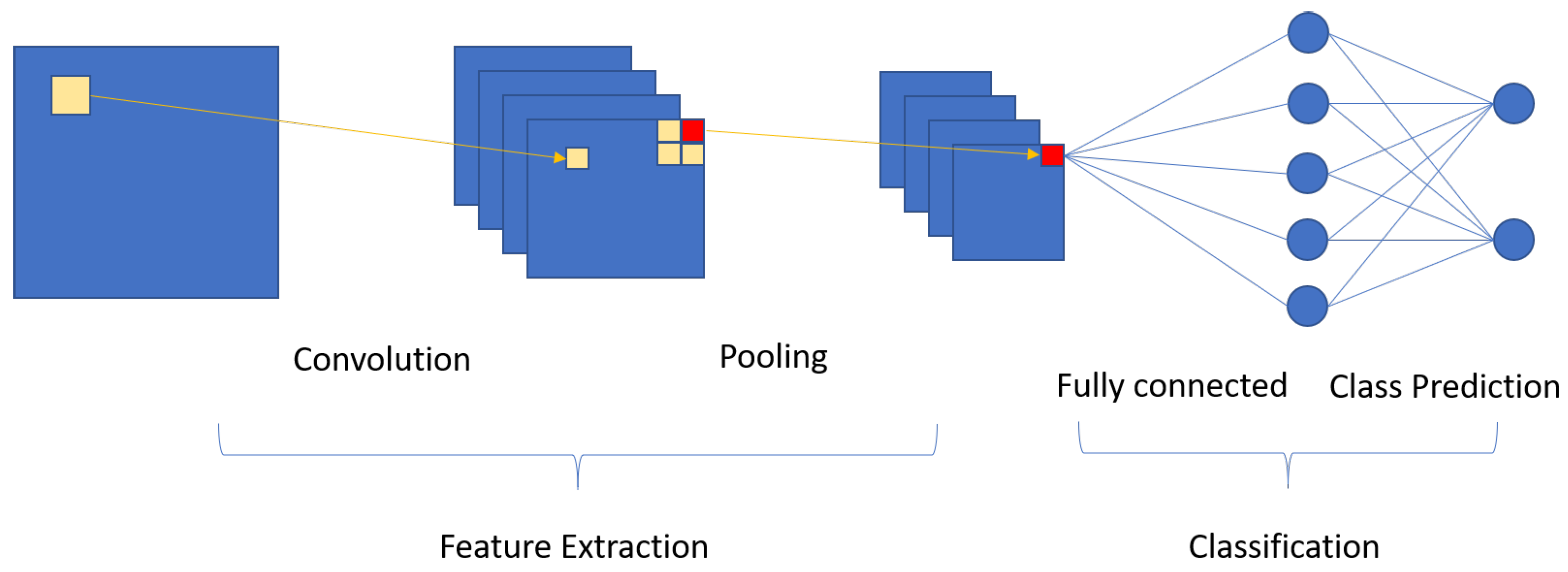
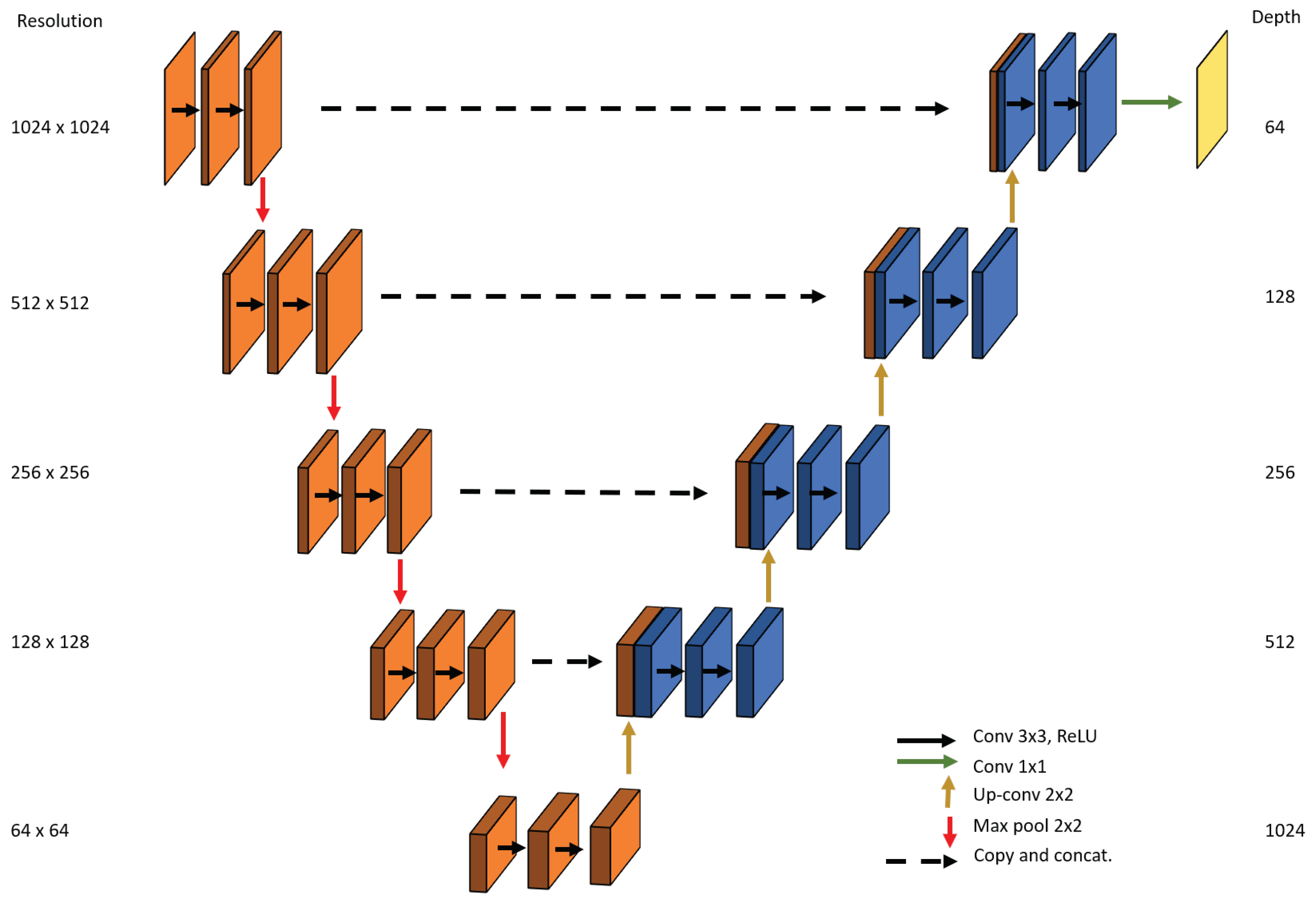
2.4. Proposed Segmentation Model

We designed a convolutional network based on the U-Net semantic segmentation architecture [25] which is a fully convolutional network that combines an encoder network that generates a dense feature map, followed by a decoder network that generates pixel-wise classification predictions. Figure 2 is a visual description of the model developed in this work and Figure 3 is flowchart describing the entire YeastNet platform. By zero-padding the tensor for every convolution operation, the output prediction tensor maintains the same size dimensions as the input image.

The network is composed of repeated motifs that consist of two 3 × 3 convolutional + ReLU layers and a resolution changing layer. In the encoder part of the network, the resolution changing layer in each motif is a 2 × 2 max-pooling layer. Four repeats of this down-sampling motif make up the encoder network. The decoder follows with four repeats of an up-sampling motif whose final layer is a transpose convolution. The final set of operations consists of two 3 × 3 convolutional + ReLU layers and a 1 × 1 convolutional layer which predicts the class probability for each pixel.

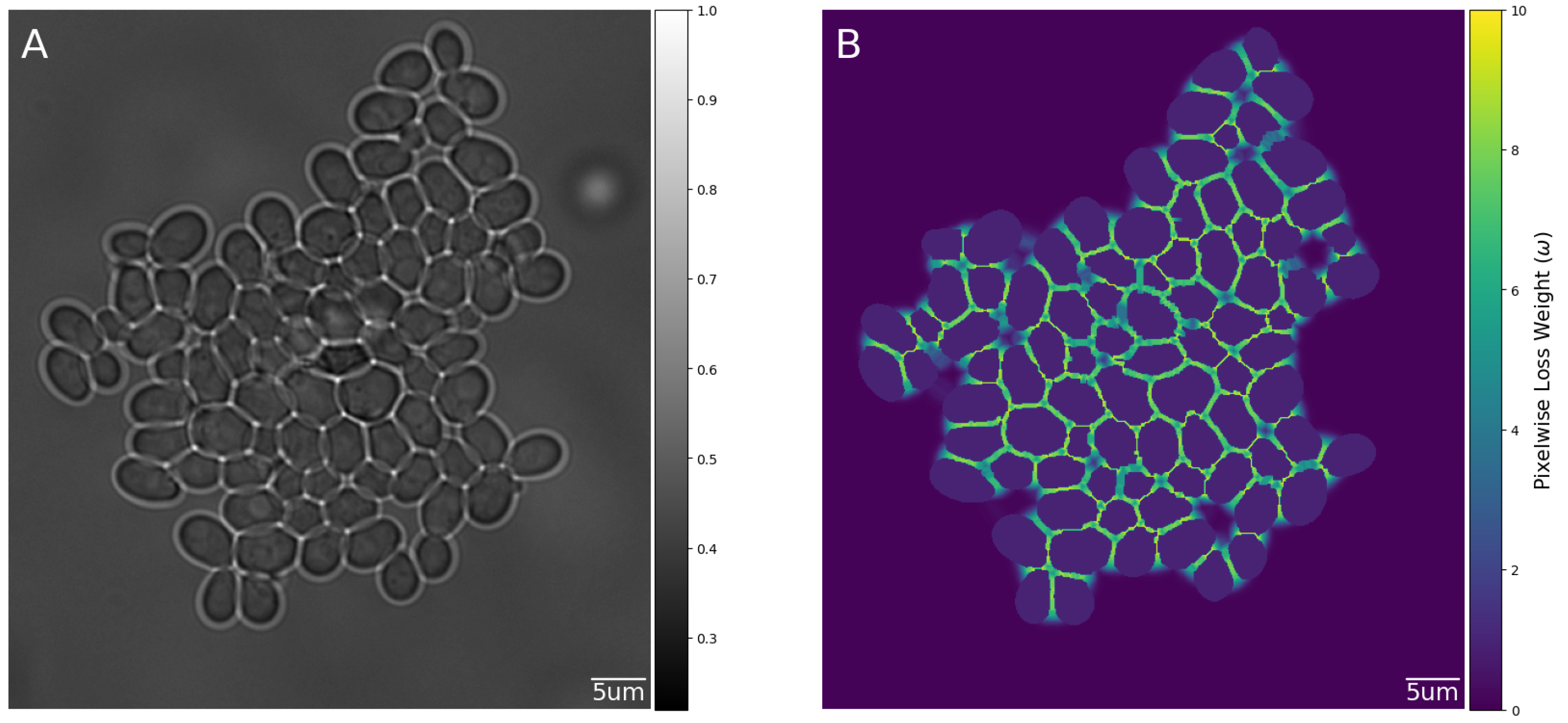
2.5. Weighted Loss Function

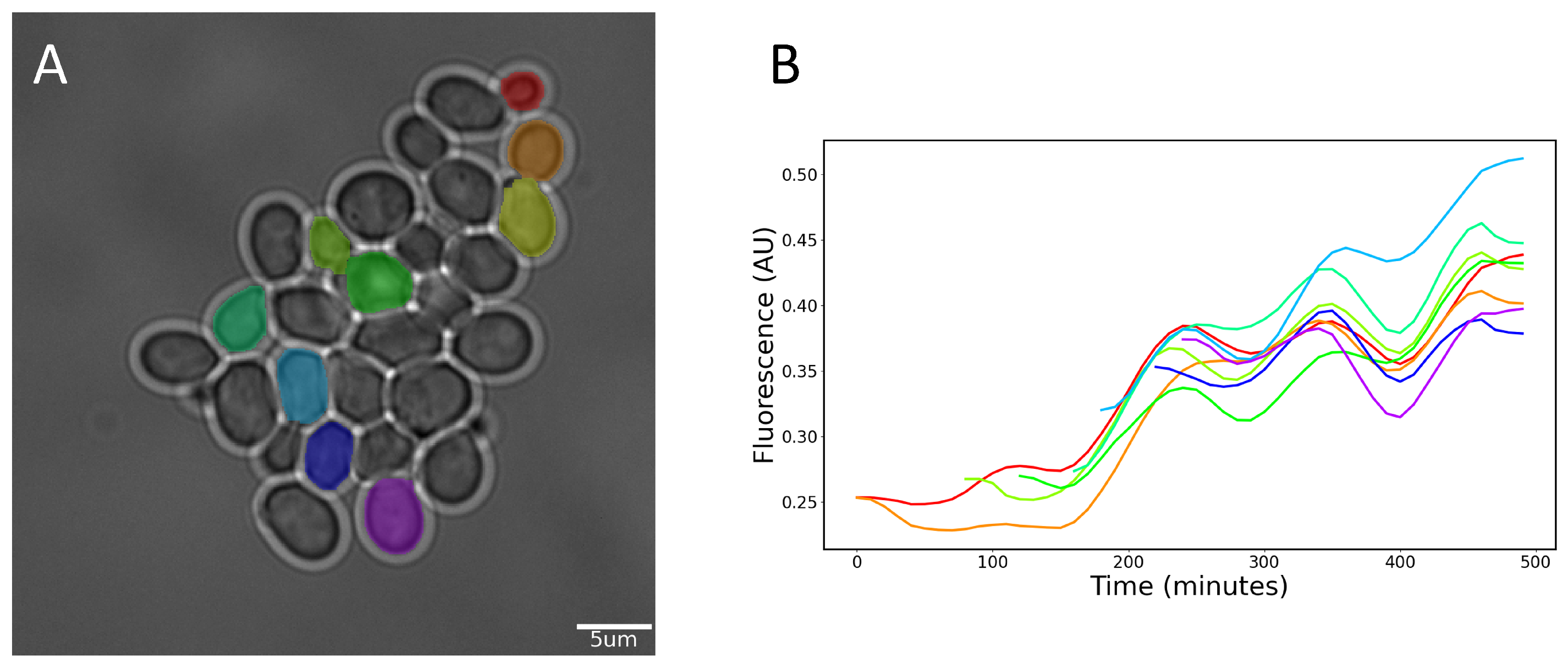
In cell segmentation, there is a very important spatial class imbalance issue that must be accounted for in any loss calculation. The number of background pixels separating cells is very small, but their correct classification is crucial for accurate segmentation and cell labeling. Without proper weighting of pixel-wise loss, a classifier can attain a very low loss by simply learning to separate colonies from the background. A weighted loss function that emphasizes the accurate prediction of the areas between cells is crucial to train the semantic segmentation of cells from background.

Cross-entropy is a very common loss function in machine learning, and it has been adapted to computer vision problems as a pixel-wise calculation. To account for the spatial class imbalance, we use a weighted pixel-wise cross-entropy loss function, first described in [25]. First, we generate a class imbalance weight matrix ($w_c$) and scale it so that the weight for every cell is 1. Next, a weight matrix favouring pixels near multiple cells with higher weights is calculated using the following equation:

$$w_p\left(x\right)=w_0·exp\left(-\frac{{(d_1\left(x\right)+d_2\left(x\right))}^2}{2{\sigma }^2}\right),$$

(1)

where x is the location of a pixel point; $d\left(x\right)$ is defined as the distance from pixel x to the nearest pixel belonging to a cell, $d_1\left(x\right)$ and $d_2\left(x\right)$ are thus the distances in pixels from the current pixel to the nearest two cells; $w_0$ and $\sigma$ are manually set parameters (in our training process, they were both set to 10). To create the final weight map, the two weight matrices are added together,

$$w\left(x\right)=w_c\left(x\right)+w_p\left(x\right),$$

(2)

to get the final weight map for a training image.

The weight map for one of the training images is shown in Figure 4. Each pixel is weighted by its proximity to cells. Therefore, the pixels between cells have a very high weight.

2.6. Cell Tracking

As cell tracking was not the main focus of this work, the algorithm used to create cell lineages is simple and effective. The problem of cell tracking is framed as a linear sum assignment optimization by calculating the combinatorial distances between all cell centroids in subsequent images. The optimization is solved using the Hungarian algorithm [43,44,45] which minimizes the sum of differences between all the paired centroids.

This algorithm is formally described for two frames (t, $t+1$) using the equation:

$$min\sum _i\sum _j{C}_{i,j}{X}_{i,j},$$

(3)

where C is a difference matrix describing the cost of pairing cell i in frame t and cell j in frame $t+1$. In our case the cost is distance between the centroids of the two cells: i and j. X is a Boolean matrix holding the assignments between cells. $X_{i,j}=1$ if i and j are assigned to be the same cell.

Tracking accuracy is defined using an F-measure statistic. The set of all true cell pairs between subsequent images is compared against the predicted cell pairs. The equation used for this metric is:

$$F=2·\frac{Precision\ast Recall}{Precision+Recall}.$$

(4)

2.7. Training Details

Training was conducted on a GPU node containing 3 16 GB NVIDIA V100 GPUs, 384 GB of RAM, and 2 18-core Intel Xeon Gold 6140 processors. Each training task used 1 V100 NVIDIA GPU, 8 GB of RAM and 8 CPU cores. We implemented this model in PyTorch 1.7 and used the Stochastic Gradient Descent optimizer. We used a learning rate of 0.1 and a momentum of 0.9 with a learning rate scheduler that reduced the learning rate by 20% after 50 epochs of accuracy stagnation. We used the ReLU activation function for every layer and the parameters were initialized using the Kaiming method [46], the default method in PyTorch.

3. Results

We compared the segmentation performance of YeastNet on our dataset to a non-trainable (manually parameterized) classic algorithm adapted from a yeast-cell-cycle research article [42]. We also compared YeastNet to CellStar [21], the current state-of-the-art tool for bright-field yeast-cell segmentation. We used the CellStar package and followed the instructions, to complete cell segmentation and tracking of our dataset. We also compared with YeastSpotter [29], a mask-RCNN deep-learning model trained for the segmentation of mammalian cell nuclei. YeastNet was trained on just training portions of our dataset and was used to demonstrate the ability of this model to generalize to unseen test samples of our datasets and all samples in YIT datasets 1 and 3. Furthermore, as a separate experiment, our model was also trained on a combination of training splits of all three datasets (we name this trained model YeastNet2) and was tested on test sets of the three datasets. The mean results obtained from 10-fold cross-validation are reported in

Table 1. 10-fold cross-validation of segmentation performance of our methods and benchmarks in terms of cell IoU. The table lists mean values with standard deviation values shown in brackets. The highest IoU for each dataset is in bold.

Method	Our Dataset	YIT Dataset 1	YIT Dataset 3
Non-trainable	0.562 (0.252)	0.585 (0.069)	0.553 (0.060)
CellStar	0.680 (0.184)	0.701 (0.070)	0.751 (0.041)
YeastSpotter	0.561 (0.109)	0.609 (0.072)	0.677 (0.043)
YeastNet	0.873 (0.020)	0.681 (0.029)	0.732 (0.012)
YeastNet2	0.883 (0.014)	0.820 (0.020)	0.855 (0.012)

. Clearly, our method achieves the highest cell IoU on our dataset. Our method also generalizes similarly to other methods, despite using a single dataset for training. Our model trained on training splits of all three datasets shows improved performance on all datasets. Figure 5 shows a visual comparison of the segmentations by the non-trainable method, CellStar, and YeastNet. (As indicated in Table 1, YeastSpotter performed worse than CellStar, thus its segmentation is not provided here.)

Our dataset contains three different bright-field images at each time point, each corresponding to a different level of focus. We compared the segmentation and tracking performance of YeastNet and CellStar separately for each level of focus. We intended to train a model to be invariant to focus level by training on all types of images (images of the same colony at different levels of focus are treated as separate training examples). To test the tracking performance, it is necessary to use the entire set of images from a time-lapse, and invariably some of these images could come from the training set. To avoid this problem, a YeastNet3 model was trained using only transformed (rotated and mirrored) images. The test set consisted of only the original images with three levels of focus.

Table 2. Cell tracking performance at different levels of focus. Focus 1: in focus, Focus 2: slightly out of focus (0.6 μm above focal plane), Focus3: more out of focus (1.2 μm above focal plane). The Cell IoU column lists mean values with standard deviation values shown in brackets, while the tracking accuracy column lists an F-measure statistic. The highest Cell IoU and tracking accuracy for each level of focus is in bold.

	Cell IoU		Tracking Accuracy
	CellStar	YeastNet3	CellStar	YeastNet3
Focus 1	0.469 (0.144)	0.888 (0.023)	0.606	0.939
Focus 2	0.771 (0.035)	0.903 (0.029)	0.858	0.922
Focus 3	0.806 (0.100)	0.917 (0.029)	0.891	0.937

shows both segmentation and tracking performance tested on the original time-course images at different levels of focus. As expected, CellStar’s segmentation performance is higher on out-of-focus images (Focuses 2 and 3) in comparison with its performance on in-focus images (Focus 1). YeastNet however has a higher cell IoU at both levels of focus, compared to CellStar. On the in-focus images, CellStar performs poorly, attaining less than a 0.5 cell IoU. Meanwhile, YeastNet obtains a cell IoU that is almost double with 0.888. YeastNet also maintains nearly the same segmentation accuracy with in-focus images as with out-of-focus images, while CellStar is over 15% lower. Thanks to its segmentation performance, YeastNet3 attains a higher tracking accuracy at every level of focus in comparison with CellStar, with the largest improvement (by 55%) at focus level 1. With the increased segmentation and tracking accuracy of YeastNet, the ultimate goal is to generate the plots as in Figure 6B from cell tracks. Each curve describes single-cell time-lapse fluorescence over a 6 h period.

4. Discussion

In this work, we present a learnable U-Net model for the segmentation of yeast cells in bright-field images. Recent advances in this field have led to the development of very accurate tools for this task but they each have several trade-offs of varying severity. Among these trade-offs are: manual and time-consuming user input, unfeasible number of z-stack image for time-lapse analysis, and expensive equipment. We demonstrate that a deep-learning approach to this problem can yield an accurate yeast-cell segmentation tool that requires minimal user input, minimal data per time point, and can be used with common and widely available imaging platforms. The high performance attained by YeastNet3 at all three levels of focus indicates that it is resistant to the segmentation errors usually caused by changes in focus. Resistance to changes in focus is a very important feature because focus drift is a significant problem that can cause many problems with image analysis [47], especially with large experiments where hundreds or thousands of images are being taken every hour.

There are several challenges in applying computer vision to this domain. A common problem with time-lapse microscopy is drift in the focus of images. The focus of bright-field images is very important because nearly all segmentation algorithms rely on the yeast cells being at a certain focal length for accurate segmentation. By using the 3 different z-stacks of each time point as separate training examples, our YeastNet model learned to detect yeast cells at different focal lengths; in essence making the trained model invariant to minor changes in the focus. A qualitative comparison of the performance on different focal lengths between our model and CellStar is shown in Figure 5A and Table 2. The higher segmentation performance leads to an increased tracking accuracy. Furthermore, the wider difference in the IoU between CellStar and YeastNet is significant for downstream applications of the cell traces. Due to variation in fluorescent protein within the cell, accurate fluorescence quantification requires entire cells to be segmented.

We also present a new, labeled dataset for training computer vision models to segment bright-field microscopy images. Since annotated data of this kind was not publicly available, only data we labeled manually could be used to train this model. Manually segmenting images to generate the datasets is laborious and due to the limited size of the dataset, we discovered that minor biases in what constitutes a cell can have many downstream effects. There is some ambiguity in what is and is not considered part of a cell, especially at different levels of focus. A computer vision model will learn to detect cells in the same way that cells are segmented in the ground-truth. Therefore, comparisons conducted with ground-truth segmentations created using different guidelines for what constitutes part of a cell, will lead to poor reported performance, even if performance appears qualitatively very high. To train a robust model, more labeled data is required. This will enable the model to generalize better to new types of datasets, including data from: different imaging modalities, lighting conditions, resolution, and magnification levels.

Analysis of time-lapse fluorescence microscopy usually involves cell segmentation followed by cell tracking. In this work, we used a simple linear sum assignment solution to the problem of cell tracking since our focus was to develop and train a network for yeast-cell segmentation. With this simple solution, YeastNet still achieves very high tracking performance. An adaptation of a recent algorithm for cell tracking such as the algorithm used in [21], or a new deep-learning approach, would lead to even higher tracking performance. Since the completion of this work, we have identified several possibilities for future improvements of YeastNet. A large new dataset has been published by Dietler et al. in support of their yeast segmentation platform YeaZ [34]. Additional training data, especially from other sources is very useful for training accurate and general models and we will use the increasing public data to improve YeastNet. We are also working on making architectural improvements to YeastNet with a focus on leveraging the recent success of adapting attention-based neural networks such as Transformers to computer vision tasks [48]. Furthermore, there is an opportunity to experiment with newly developed loss functions such as the soft Dice and soft Jaccard loss functions. Analyses comparing these loss functions to the cross-entropy and class-weighted cross-entropy loss functions has been done recently [49] and shown that model performance is higher when using soft Dice and soft Jaccard. Although this analysis does not investigate the spatially weighted cross-entropy introduced in [25] that we use in this work, determining how it fits into the landscape of biomedical imaging semantic segmentation is an important question that we will investigate to further improve YeastNet performance.

5. Conclusions

We designed YeastNet to improve the accuracy of identifying individual S. cerevisiae cells from bright-field microscopy images. Our model is based on the U-Net semantic segmentation architecture and it was trained using a manually labeled dataset. YeastNet segments bright-field images by generating pixel-wise predictions between background and cell classes. We compared YeastNet to a classic method and the current state-of-the-art tool for general S. cerevisiae segmentation and tracking. We achieve higher performance in every metric used: intersection over union, segmentation accuracy, and tracking accuracy.

We also present a new dataset, consisting of 150 bright-field microscopy images of budding yeast. This dataset consists of 50 fields of view of a growing colony, taken at 3 levels of focus, as well as, manually segmented ground-truth segmentation masks. This publicly available dataset for bright-field microscopy segmentation of yeast adds to the limited public data, and we hope it is used to advance research in this domain.

References

1. Elowitz, M.B.; Levine, A.J.; Siggia, E.D.; Swain, P.S. Stochastic gene expression in a single cell. Science 2002, 297, 1183–1186. [Google Scholar] [CrossRef] [Green Version]
2. Bintu, L.; Yong, J.; Antebi, Y.E.; McCue, K.; Kazuki, Y.; Uno, N.; Oshimura, M.; Elowitz, M.B. Dynamics of epigenetic regulation at the single-cell level. Science 2016, 351, 720–724. [Google Scholar] [CrossRef] [PubMed] [Green Version]
3. Andersen, J.B.; Sternberg, C.; Poulsen, L.K.; Bjørn, S.P.; Givskov, M.; Molin, S. New unstable variants of green fluorescent protein for studies of transient gene expression in bacteria. Appl. Environ. Microbiol. 1998, 64, 2240–2246. [Google Scholar] [CrossRef] [Green Version]
4. Shaner, N.C.; Steinbach, P.A.; Tsien, R.Y. A guide to choosing fluorescent proteins. Nat. Methods 2005, 2, 905. [Google Scholar] [CrossRef]
5. Gordon, A.; Colman-Lerner, A.; Chin, T.E.; Benjamin, K.R.; Richard, C.Y.; Brent, R. Single-cell quantification of molecules and rates using open-source microscope-based cytometry. Nat. Methods 2007, 4, 175. [Google Scholar] [CrossRef] [PubMed]
6. Prewitt, J.M.; Mendelsohn, M.L. The analysis of cell images. Ann. N. Y. Acad. Sci. 1966, 128, 1035–1053. [Google Scholar] [CrossRef]
7. Otsu, N. A threshold selection method from gray-level histograms. IEEE Trans. Syst. Man Cybern. 1979, 9, 62–66. [Google Scholar] [CrossRef] [Green Version]
8. Jianzhuang, L.; Wenqing, L.; Yupeng, T. Automatic thresholding of gray-level pictures using two-dimension Otsu method. In Proceedings of the 1991 International Conference on Circuits and Systems, Shenzhen, China, 16–17 June 1991; pp. 325–327. [Google Scholar]
9. Bradley, D.; Roth, G. Adaptive thresholding using the integral image. J. Graph. Tools 2007, 12, 13–21. [Google Scholar] [CrossRef]
10. Li, Y.; Sun, J.; Tang, C.K.; Shum, H.Y. Lazy snapping. ACM Trans. Graph. (ToG) 2004, 23, 303–308. [Google Scholar] [CrossRef]
11. Rother, C.; Kolmogorov, V.; Blake, A. “GrabCut” interactive foreground extraction using iterated graph cuts. ACM Trans. Graph. (TOG) 2004, 23, 309–314. [Google Scholar] [CrossRef]
12. Protiere, A.; Sapiro, G. Interactive image segmentation via adaptive weighted distances. IEEE Trans. Image Process. 2007, 16, 1046–1057. [Google Scholar] [CrossRef] [PubMed] [Green Version]
13. Kass, M.; Witkin, A.; Terzopoulos, D. Snakes: Active contour models. Int. J. Comput. Vis. 1988, 1, 321–331. [Google Scholar] [CrossRef]
14. Caselles, V.; Kimmel, R.; Sapiro, G. Geodesic active contours. Int. J. Comput. Vis. 1997, 22, 61–79. [Google Scholar] [CrossRef]
15. Chan, T.F.; Vese, L.A. Active contours without edges. IEEE Trans. Image Process. 2001, 10, 266–277. [Google Scholar] [CrossRef] [Green Version]
16. Beucher, S. Use of watersheds in contour detection. In Proceedings of the International Workshop on Image Processing, Astrophysics, Trieste, 4–8 June 1979. [Google Scholar]
17. Meyer, F. Topographic distance and watershed lines. Signal Process. 1994, 38, 113–125. [Google Scholar] [CrossRef]
18. Doncic, A.; Eser, U.; Atay, O.; Skotheim, J.M. An algorithm to automate yeast segmentation and tracking. PLoS ONE 2013, 8, e57970. [Google Scholar] [CrossRef]
19. Wood, N.E.; Doncic, A. A fully-automated, robust, and versatile algorithm for long-term budding yeast segmentation and tracking. PLoS ONE 2019, 14, e0206395. [Google Scholar] [CrossRef] [Green Version]
20. Bredies, K.; Wolinski, H. An active-contour based algorithm for the automated segmentation of dense yeast populations on transmission microscopy images. Comput. Vis. Sci. 2011, 14, 341–352. [Google Scholar] [CrossRef]
21. Versari, C.; Stoma, S.; Batmanov, K.; Llamosi, A.; Mroz, F.; Kaczmarek, A.; Deyell, M.; Lhoussaine, C.; Hersen, P.; Batt, G. Long-term tracking of budding yeast cells in brightfield microscopy: CellStar and the Evaluation Platform. J. R. Soc. Interface 2017, 14, 20160705. [Google Scholar] [CrossRef]
22. LeCun, Y.; Bottou, L.; Bengio, Y.; Haffner, P. Gradient-based learning applied to document recognition. Proc. IEEE 1998, 86, 2278–2324. [Google Scholar] [CrossRef] [Green Version]
23. Krizhevsky, A.; Sutskever, I.; Hinton, G.E. ImageNet classification with deep convolutional neural networks. In Proceedings of the Advances in Neural Information Processing Systems, Lake Tahoe, CA, USA, 3–8 December 2012; pp. 1097–1105. [Google Scholar]
24. Long, J.; Shelhamer, E.; Darrell, T. Fully convolutional networks for semantic segmentation. In Proceedings of the IEEE Conference on Computer Vision and Pattern Recognition, Boston, IL, USA, 8–10 June 2015; pp. 3431–3440. [Google Scholar]
25. Ronneberger, O.; Fischer, P.; Brox, T. U-Net: Convolutional networks for biomedical image segmentation. In Proceedings of the International Conference on Medical Image Computing and Computer Assisted Intervention, Munich, Germany, 5–9 October 2015; pp. 234–241. [Google Scholar]
26. Van Valen, D.; Kudo, T.; Lane, K.M.; Macklin, D.N.; Quach, N.T.; DeFelice, M.M.; Maayan, I.; Tanouchi, Y.; Ashley, E.A.; Covert, M.W. Deep Learning Automates the Quantitative Analysis of Individual Cells in Live-Cell Imaging Experiments. PLoS Comput. Biol. 2016, 12, 1–24. [Google Scholar] [CrossRef] [Green Version]
27. Aydin, A.S.; Dubey, A.; Dovrat, D.; Aharoni, A.; Shilkrot, R. CNN based yeast cell segmentation in multi-modal fluorescent microscopy data. In Proceedings of the 2017 IEEE Conference on Computer Vision and Pattern Recognition Workshops (CVPRW), Honolulu, HI, USA, 21–26 July 2017; pp. 753–759. [Google Scholar]
28. Badrinarayanan, V.; Kendall, A.; Cipolla, R. Segnet: A deep convolutional encoder-decoder architecture for image segmentation. IEEE Trans. Pattern Anal. Mach. Intell. 2017, 39, 2481–2495. [Google Scholar] [CrossRef]
29. Lu, A.X.; Zarin, T.; Hsu, I.S.; Moses, A.M. YeastSpotter: Accurate and parameter-free web segmentation for microscopy images of yeast cells. Bioinformatics 2019, 35, 4525–4527. [Google Scholar] [CrossRef] [Green Version]
30. Ljosa, V.; Caie, P.D.; Ter Horst, R.; Sokolnicki, K.L.; Jenkins, E.L.; Daya, S.; Roberts, M.E.; Jones, T.R.; Singh, S.; Genovesio, A.; et al. Comparison of methods for image-based profiling of cellular morphological responses to small-molecule treatment. J. Biomol. Screen. 2013, 18, 1321–1329. [Google Scholar] [CrossRef] [PubMed] [Green Version]
31. Lugagne, J.B.; Lin, H.; Dunlop, M.J. DeLTA: Automated cell segmentation, tracking, and lineage reconstruction using deep learning. PLoS Comput. Biol. 2020, 16, e1007673. [Google Scholar] [CrossRef] [Green Version]
32. Zhang, M.; Li, X.; Xu, M.; Li, Q. RBC semantic segmentation for sickle cell disease based on deformable U-Net. In Proceedings of the International Conference on Medical Image Computing and Computer-Assisted Intervention, Granada, Spain, 16–20 September 2018; pp. 695–702. [Google Scholar]
33. Dai, J.; Qi, H.; Xiong, Y.; Li, Y.; Zhang, G.; Hu, H.; Wei, Y. Deformable convolutional networks. In Proceedings of the IEEE International Conference on Computer Vision, Venice, Italy, 22–29 October 2017; pp. 764–773. [Google Scholar]
34. Dietler, N.; Minder, M.; Gligorovski, V.; Economou, A.M.; Joly, D.A.H.L.; Sadeghi, A.; Chan, C.H.M.; Koziński, M.; Weigert, M.; Bitbol, A.F.; et al. A convolutional neural network segments yeast microscopy images with high accuracy. Nat. Commun. 2020, 11, 1–8. [Google Scholar] [CrossRef] [PubMed]
35. Prangemeier, T.; Wildner, C.; Françani, A.O.; Reich, C.; Koeppl, H. Multiclass yeast segmentation in microstructured environments with deep learning. In Proceedings of the 2020 IEEE Conference on Computational Intelligence in Bioinformatics and Computational Biology (CIBCB), Via del Mar, Chile, 27–29 October 2020; pp. 1–8. [Google Scholar]
36. Kong, Y.; Li, H.; Ren, Y.; Genchev, G.Z.; Wang, X.; Zhao, H.; Xie, Z.; Lu, H. Automated yeast cells segmentation and counting using a parallel U-Net based two-stage framework. OSA Contin. 2020, 3, 982–992. [Google Scholar] [CrossRef]
37. Haralick, R.; Shapiro, L. Computer and Robot Vision; Number v. 1 in Computer and Robot Vision; Addison-Wesley Publishing Company: Reading, MA, USA, 1992. [Google Scholar]
38. Uhlendorf, J.; Miermont, A.; Delaveau, T.; Charvin, G.; Fages, F.; Bottani, S.; Batt, G.; Hersen, P. Long-term model predictive control of gene expression at the population and single-cell levels. Proc. Natl. Acad. Sci. USA 2012, 109, 14271–14276. [Google Scholar] [CrossRef] [PubMed] [Green Version]
39. Edelstein, A.D.; Tsuchida, M.A.; Amodaj, N.; Pinkard, H.; Vale, R.D.; Stuurman, N. Advanced methods of microscope control using μManager software. J. Biol. Methods 2014, 1, e10. [Google Scholar] [CrossRef] [PubMed] [Green Version]
40. Schneider, C.A.; Rasband, W.S.; Eliceiri, K.W. NIH Image to ImageJ: 25 years of image analysis. Nat. Methods 2012, 9, 671–675. [Google Scholar] [CrossRef]
41. Schindelin, J.; Arganda-Carreras, I.; Frise, E.; Kaynig, V.; Longair, M.; Pietzsch, T.; Preibisch, S.; Rueden, C.; Saalfeld, S.; Schmid, B.; et al. Fiji: An open-source platform for biological-image analysis. Nat. Methods 2012, 9, 676. [Google Scholar] [CrossRef] [Green Version]
42. Ricicova, M.; Hamidi, M.; Quiring, A.; Niemistö, A.; Emberly, E.; Hansen, C.L. Dissecting genealogy and cell cycle as sources of cell-to-cell variability in MAPK signaling using high-throughput lineage tracking. Proc. Natl. Acad. Sci. USA 2013, 110, 11403–11408. [Google Scholar] [CrossRef] [Green Version]
43. Kuhn, H. The Hungarian method for the assignment problem. Nav. Res. Logist. Q. 1955, 2, 83–97. [Google Scholar] [CrossRef] [Green Version]
44. Munkres, J. Algorithms for the assignment and transportation problems. J. Soc. Ind. Appl. Math. 1957, 5, 32–38. [Google Scholar] [CrossRef] [Green Version]
45. Kachouie, N.; Fieguth, P. Extended-Hungarian-JPDA: Exact Single-Frame Stem Cell Tracking. IEEE Trans. Biomed. Eng. 2007, 54, 2011–2019. [Google Scholar] [CrossRef] [PubMed]
46. He, K.; Zhang, X.; Ren, S.; Sun, J. Delving deep into rectifiers: Surpassing human-level performance on imagenet classification. In Proceedings of the IEEE International Conference on Computer Vision, Las Condes, Chile, 11–18 December 2015; pp. 1026–1034. [Google Scholar]
47. Kreft, M.; Stenovec, M.; Zorec, R. Focus-drift correction in time-lapse confocal imaging. Ann. N. Y. Acad. Sci. 2005, 1048, 321–330. [Google Scholar] [CrossRef] [PubMed]
48. Dosovitskiy, A.; Beyer, L.; Kolesnikov, A.; Weissenborn, D.; Zhai, X.; Unterthiner, T.; Dehghani, M.; Minderer, M.; Heigold, G.; Gelly, S.; et al. An Image is Worth 16x16 Words: Transformers for Image Recognition at Scale. In Proceedings of the International Conference on Learning Representations, Vienna, Austria, 4 May 2021. [Google Scholar]
49. Bertels, J.; Eelbode, T.; Berman, M.; Vandermeulen, D.; Maes, F.; Bisschops, R.; Blaschko, M.B. Optimizing the dice score and jaccard index for medical image segmentation: Theory and practice. In Proceedings of the International Conference on Medical Image Computing and Computer-Assisted Intervention, Shenzen, China, 13–17 October 2019; pp. 92–100. [Google Scholar]
Figure 1. A visual description of simple Convolutional Neural Network (CNN). Convolution layers produce feature maps that get down-sampled by max-pooling layers. Combinations of these two layer types make up the feature extraction part of a CNN. A fully connected layer reads the output of the feature extraction and outputs a class prediction probability for every class in the data.
Applsci 11 02692 g001
Figure 2. A visual description of the modified U-Net architecture applied in this work. Images in the down-sampling stage are orange and images in the up-sampling stage are blue. The pixel-wise class prediction output is yellow. Solid horizontal arrows indicate convolutional operations that do not change the height or width of the inference tensor. Vertical arrows indicate operations that reduce or increase the size of the inference tensor. Skip connections are represented by a dashed black arrow. The resolution of each tensor is shown on the left, and the feature depth at each level is shown on the right. The depth corresponds to the layer depth of each individual tensor in the row, tensors that result from skip connections have twice the depth. The output depth corresponds to the number of classes in the classification problem, in our case the dimensions of the output is 1024 × 1024 × 2.
Applsci 11 02692 g002
Figure 3. Flowchart diagram describing the YeastNet platform from start to finish. Orange parallelograms indicate objects such as images or arrays, green diamonds indicate decision points and blue rectangles indicate processes. The data construction section involves the acquisition of microscopy images, manual labeling of cells to produce ground-truth masks, as well as the calculation of loss weight maps. The training loop runs for 1000 epochs, with a validation step at the end of every epoch. If the intersection over union (IoU) accuracy of the network on the validation dataset is higher than the previous best parameter set, the new parameters are saved. In this sequence, the YeastNet parameters that achieve the highest IoU obtained on the validation dataset after 1000 epochs are the saved parameters. The final segment shows the tracking algorithm used in YeastNet. By seeding the watershed algorithm with highly accurate markers obtained from YeastNet, instance labeled cell masks can be obtained and used for tracking using the Hungarian algorithm. The output is therefore an instance labeled and tracked segmentation mask for every microscopy image input into YeastNet.
Applsci 11 02692 g003
Figure 4. (B) The weighted loss matrix used to bias the pixel-wise cross-entropy loss and the (A) microscopy image for which it was generated. The pixel color in (B) indicates the final weight taking into account class imbalance and proximity to cells. The image was obtained using a 60X oil immersion objective. A 5 μm scale bar is presents to show the scale of yeast cells.
Applsci 11 02692 g004
Figure 5. Cell segmentation mask of the same colony at different levels of focus. From top to bottom the input images shown are: in focus, slightly out of focus (0.6 μm above focal plane), more out of focus (1.2 μm above focal plane). From left to right: cropped input image, and segmentations using the non-trainable method, CellStar and YeastNet. Images were obtained using a 60X oil immersion objective. A 5 μm scale bar is presents to show the scale of yeast cells.
Applsci 11 02692 g005
Figure 6. (A) Bright-Field Microscopy image from our dataset. The cells whose fluorescence profiles are plotted in (B) match the color-coding in (A). (B) Single-cell fluorescence tracking, generated by YeastNet, to study dynamic gene expression. Each curve is a time-lapse mean pixel fluorescence measure describing the protein abundance of a dynamically expressed gene in an individually tracked cell. Each plot was smoothed using a window of length 5. The image was obtained using a 60× oil immersion objective. A 5 μm scale bar is presents to show the scale of yeast cells.
Applsci 11 02692 g006