On the Calculation of System Entropy in Nonlinear Stochastic Biological Networks

Abstract

Biological networks are open systems that can utilize nutrients and energy from their environment for use in their metabolic processes, and produce metabolic products. System entropy is defined as the difference between input and output signal entropy, i.e., the net signal entropy of the biological system. System entropy is an important indicator for living or non-living biological systems, as biological systems can maintain or decrease their system entropy. In this study, system entropy is determined for the first time for stochastic biological networks, and a computation method is proposed to measure the system entropy of nonlinear stochastic biological networks that are subject to intrinsic random fluctuations and environmental disturbances. We find that intrinsic random fluctuations could increase the system entropy, and that the system entropy is inversely proportional to the robustness and stability of the biological networks. It is also determined that adding feedback loops to shift all eigenvalues to the farther left-hand plane of the complex s-domain could decrease the system entropy of a biological network.

1. Introduction

Entropy is a measure of the randomness or disorder of a physical system due to intrinsic random fluctuations and environmental disturbances [1,2,3]. According to the second law of thermodynamics in a thermally isolated system, entropy typically tends to increase, i.e., entropy describes the dispersion of energy and the natural tendency of spontaneous change toward states with higher entropy [4,5,6,7]. However, biological systems can absorb nutrients and energy from the external environment for use in metabolic processes, producing metabolites to maintain life. Since these biological systems can exchange material and energy with their environments to maintain their stability and structure, they are open systems, i.e., their entropy can be maintained by exchanging materials and energy with their environment. The maintenance of entropy is an important indicator separating biological systems from non-living systems. As pointed out by Schrödinger, biological systems consume negative entropy to maintain the entropy used for their maintenance [8,9].

Biosystems are open irreversible statistical thermodynamic systems [10,11,12,13,14]. It is still difficult to measure the entropy of biological systems however, because these are always stochastic dynamic systems [10,11,12]. At present, no efficient method exists for use in calculating the entropy of nonlinear stochastic networks [1,2,3,8,13,14,15]. When a nonlinear stochastic network is driven by white noise, the entropy of the biological network is a measure of its randomness, which is characterized by the covariance of the state variables of the biological network [2,6]. The entropy of a nonlinear stochastic biological network is therefore denoted as the normalized randomness of the driven white noise [8,16,17,18,19,20,21,22,23,24,25]. The entropy of a biological network is in fact a systematic property [6]. It is very difficult to measure systematic randomness in order to calculate the entropy of a biological network directly. In this study, we describe the system entropy of a stochastic system in terms of the input signal entropy minus the output signal entropy (i.e., the net signal entropy of the biological network), introducing an indirect method for measuring the system entropy of a stochastic biological system. The purpose of this paper is to emphasize that system entropy is a systematic characteristic of biological systems. Based on systems theory, we could calculate the system entropy of biological systems from their system matrices. Like lowpass filters, we could understand their system properties from their transfer functions or frequency response functions, without measuring their input/output signals. Under a systematic Hamilton-Jacobi inequality (HJI) -constraint, we were able to minimize the upper bound of the system entropy to approach the real system entropy of a nonlinear biological network. The entropy measurement problem of nonlinear stochastic networks can therefore be transformed to an HJI-constrained optimization problem. It was found that intrinsic random parameter fluctuations increase the system entropy of a biological network, while a feedback loop with all eigenvalues shifted to the farther left-hand plane of the complex s-domain could decrease the system entropy and stabilize the biological network.

At present, there is no efficient method for solving the HJI-constrained optimization problem in the calculation of the system entropy of a nonlinear stochastic biological network. In this study, based on a global linearization technique, several linearized biological networks are interpolated at certain operation points to approximate the nonlinear biological network. In this way, the HJI could be interpolated by a set of linear matrix inequalities (LMIs) [26]. In this case, LMIs-constrained optimization could replace HJI-constrained optimization for measuring the system entropy of nonlinear biological networks. Furthermore, the relationship between system entropy and robustness and stability, as well as the sensitivity of a biological network, are also discussed to obtain a more systematic insight into the system entropy. We found that more stable biological networks correspond to lower system entropies. A biological network with more robustness or less sensitivity will also exhibit lower system entropy. This observation has also been confirmed by previous findings [27,28,29,30,31,32,33,34,35,36,37,38,39,40]. Furthermore, it can be observed that the system entropy of a biological network is a measure of the network response to environmental disturbances [41,42,43,44,45,46,47]. Lower system entropy implies less sensitivity to environment disturbances, and vice versa. With the help of the LMI toolbox available in the Matlab software package, we could easily solve the corresponding LMIs-constrained optimization problem to measure the system entropy of a nonlinear biological network. Finally, two in silico examples of nonlinear biological networks are given to illustrate the system-entropy measurement procedure, and to gain a greater insight into the systematic responses of living systems to their environments.

2. Results and Discussion

2.1. On the Measurement of System Entropy in Linear Stochastic Biological Networks

First, for simplicity, we consider a linear biological network with the following stoichiometric equation (Figure 1):

$$\begin{array}{l}\dot{X}\left(t\right)=AX\left(t\right)+Bv\left(t\right)\\ y\left(t\right)=CX\left(t\right)\end{array}$$

(1)

where X(t) = [x₁(t) ... x_n(t)]^T denotes the state vector of the biological network with n species, v(t) = [v₁(t) ... v_n(t)]^T represents the network input, y(t) indicates the network output. A, B, and C respectively denote the system interaction matrix, input coupling matrix and output coupling matrix of the linear biological network as follows:

$$A=\left[\begin{array}{ccc}{a}_{11}& \cdots & a_{1n}\\ ⋮& \ddots & ⋮\\ a_{n1}& \cdots & a_{nn}\end{array}\right]\text{, }B=\left[\begin{array}{ccc}{b}_{11}& \cdots & b_{1m}\\ ⋮& \ddots & ⋮\\ b_{n1}& \cdots & b_{nm}\end{array}\right],C=\left[\begin{array}{ccc}{c}_{11}& \cdots & c_{1n}\\ ⋮& \ddots & ⋮\\ c_{l1}& \cdots & c_{ln}\end{array}\right]$$

If all state variables of the biological network are considered as the network output, C = diag [C₁₁ ... C_ln]; if the last state x_n(t) is the only network output, C = [0 ... 0 C_ln]. The randomness of the output or input signals can be perceived as the dispersal of the random signals [6], i.e., randomness of output signal is represented as $r_o=E\left\{{\displaystyle {\int }_0^T{y}^T\left(t\right)y\left(t\right)dt}/T\right\}$ when the randomness of input white noise is $r_i=E\left\{{\displaystyle {\int }_0^T{v}^T\left(t\right)v\left(t\right)dt}/T\right\}$ where $E\{·\}$ denotes the expectation of $·$ and T is the time period of input white noise v(t), i.e., v(t) is within the time interval $[0,T)$. The entropy of input noise or output signal is defined as the logarithm of its randomness [6,8], i.e., the entropy of input noise $s_i=-\log E\left\{{\displaystyle {\int }_0^T{v}^T\left(t\right)v\left(t\right)dt}/T\right\}$ and the entropy of output signal $s_o=-\log E\left\{{\displaystyle {\int }_0^T{y}^T\left(t\right)y\left(t\right)dt}/T\right\}$. Therefore, the entropy of linear stochastic biological system (1) is the difference between output signal entropy and input signal entropy with zero initial state condition X(0) = 0, i.e., the system entropy is defined as the net signal entropy of biological system:

$$s=s_i-s_o=\log E\left\{\frac{1}{T}{\displaystyle {\int }_0^T{y}^T\left(t\right)y\left(t\right)dt}\right\}-\log E\left\{\frac{1}{T}{\displaystyle {\int }_0^T{v}^T\left(t\right)v\left(t\right)dt}\right\}$$

or:

$$s=\log \frac{E\left\{\frac{1}{T}{\displaystyle {\int }_0^T{y}^T\left(t\right)y\left(t\right)dt}\right\}}{E\left\{\frac{1}{T}{\displaystyle {\int }_0^T{v}^T\left(t\right)v\left(t\right)dt}\right\}}=\log \frac{E\left\{{\displaystyle {\int }_0^T{y}^T\left(t\right)y\left(t\right)dt}\right\}}{E\left\{{\displaystyle {\int }_0^T{v}^T\left(t\right)v\left(t\right)dt}\right\}},X\left(0\right)=0$$

(2)

Let us denote the system randomness r as $r\triangleq E\left\{{\displaystyle {\int }_0^T{y}^T\left(t\right)y\left(t\right)dt}\right\}/E\left\{{\displaystyle {\int }_0^T{v}^T\left(t\right)v\left(t\right)dt}\right\},X\left(0\right)=0$, then the entropy of the linear stochastic system is the logarithm of the randomness of the system, i.e., $s\triangleq \log r$. If we can measure system randomness r, its logarithm is the system entropy s. It is seen that if the input signal randomness is less than the output signal randomness (i.e., r < 1), system entropy is negative (i.e., s < 0). In this situation, biological networks can absorb biomass and energy from the environment by metabolic processes obtaining negative entropy to improve the orderly structure of the biology network. As a result, system entropy will decrease naturally. Obviously, this definition of system entropy match the Schrödinger’s claim that biological life is maintained by negative entropy. The system entropy is a modification of the entropy in systems theory [6,8,15]. We add the logarithm to it to more meet the conventional information entropy so that is more convenient for us to discuss system entropy in biological system from the systematic perspective. If the biological network disperses biomass and energy to the environment (i.e., r > 1), the system entropy s is positive (i.e., s >0). In this situation, the biological network will obtain the entropy and its orderly structure will be destroyed.

Figure 1. A simple linear stochastic biological network with stochastic dynamic model in Equation (1).

Figure 1. A simple linear stochastic biological network with stochastic dynamic model in Equation (1).

In general, it is difficult to calculate the system entropy s in (2) for the linear biological network in Equation (1) directly. In this study, an indirect method is proposed to calculate the system entropy s in Equation (2) via the system characteristics of the biological network. Let us denote the upper bound $\overline{r}$ of the system randomness as follows:

$$r=\frac{E\left\{{\displaystyle {\int }_0^T{y}^T\left(t\right)y\left(t\right)dt}\right\}}{E\left\{{\displaystyle {\int }_0^T{v}^T\left(t\right)v\left(t\right)dt}\right\}}\le \overline{r}\text{ or }E\left\{{\displaystyle {\int }_0^T{y}^T\left(t\right)y\left(t\right)dt}\right\}\le \overline{r}E\left\{{\displaystyle {\int }_0^T{v}^T\left(t\right)v\left(t\right)dt}\right\},X\left(0\right)=0$$

(3)

We will firstly estimate the upper bound $\overline{r}$ of the system randomness in Equation (3) and then decrease $\overline{r}$ as small a value as possible to approach the system randomness of the biological network. Then we get the following result.

Remark 1. If the initial condition is X(0) ≠ 0 in Equation (1), then the energy of initial state X(0) should be considered into the system randomness of biological system and Equation (3) should be modified as:

$$r=\frac{E\left\{{\displaystyle {\int }_0^T{y}^T\left(t\right)y\left(t\right)dt}\right\}}{V\left(X\left(0\right)\right)+E\left\{{\displaystyle {\int }_0^T{v}^T\left(t\right)v\left(t\right)dt}\right\}},X\left(0\right)\ne 0$$

for some positive energy function V(X) > 0 and V(0) = 0, i.e., the randomness of the initial state of the biological network should be added to the randomness of input signal. In this situation, the system entropy should be modified as follows

$$s=\log \frac{E\left\{{\displaystyle {\int }_0^T{y}^T\left(t\right)y\left(t\right)dt}\right\}}{V\left(X\left(0\right)\right)+E\left\{{\displaystyle {\int }_0^T{v}^T\left(t\right)v\left(t\right)dt}\right\}},X\left(0\right)\ne 0$$

for some positive energy function V(X) > 0, i.e., the net signal entropy in Equation (2) should take account of the effect of the initial state X(0). In general, V(X(t)) is chosen as the Lyapunov function V(X(t)) = X^T(t)PX(t) for some positive symmetric matrix P > 0.

Definition 1. The linear biological system in Equation (1) is called stable if all the eigenvalues of A are in the left-hand side of the s-domain, i.e., the real parts of eigenvalues Re{λ_i(A)} ≤ 0 for all i.

Proposition 1.

The system randomness of the linear biological network in Equation (1) has an upper bound $\overline{r}$ if the following LMI has a positive solution P = P^T > 0.

$$\left[\begin{array}{cc}PA+A^{T}P+C^{T}C& PB\\ B^{T}P& -\overline{r}I\end{array}\right]\le 0$$

(4)

Proof.

See Appendix A.

From Equation (3), it is seen that $\overline{r}$ is the upper bound of the system randomness r. From the Proposition 1, the system randomness of the linear biological network Equation (1) can be estimated by solving the following LMI-constrained optimization problem:

$$r=\underset{P>0}{\min }\overline{r}\mathrm{ subject\; to\; LMI\; in\; (4)}$$

(5)

The above LMI-constrained optimization problem can be easily solved by decreasing $\overline{r}$ in LMI Equation (4) until there exists no positive definite symmetric matrix P, which could be easily performed with the help of the LMI toolbox available in the Matlab software package. After solving the LMI-constrained optimization for system randomness r in Equation (5), we could obtain the system entropy of the linear stochastic system in Equation (1) as $s=\log r$. Since LMI in Equation (4) is characterized by system matrices A, B and C, the system randomness r or system entropy s measured by solving the LMI-constrained optimization problem in Equation (5) is completely dependent on system matrices A, B and C in Equation (1).

Remark 2.

(i)

The LMI in Equation (4) is equivalent to the following Riccati-like equation through the Schur complement [15]:

$$PA+A^{T}P+C^{T}C+\frac{1}{\overline{r}}PB{B}^{T}P\le 0$$

(6)

(ii)

Obtaining the system randomness r by solving the LMI-constrained optimization problem in Equation (5), the Riccati-like equation in Equation (6) could be replaced by:

$$C^{T}C+\frac{1}{r}PB{B}^{T}P\le -\left(PA+A^{T}P\right)$$

(7)

From the Riccati-like inequality in Equation (7), it is clear that the system randomness r and also the system entropy s are all dependent on the system parameters A, B and C. Obviously, the system randomness r or entropy s is a measurement of systematic characteristic. Since the last term in the right-hand side of the inequality Equation (7) is positive, it is seen that if the eigenvalues of A are all located at the farther left-hand side of s-domain (i.e., the real parts of eigenvalues are more negative or the loops of biological system are with more strength from the systematic perspective) (Figure 2), the biological network in Equation (1) is with less system randomness r and lower system entropy s. If the eigenvalues of A are all located near the imaginary axis (i.e., less negative), in order to maintain the inequality in Equation (7), the system randomness r or system entropy s must be large enough. In summary, biological systems with more stability are with more ability to maintain its system structure (or phenotype) and therefore is with less system randomness or entropy, and vice versa.

(iii)

From the Riccati-like inequality in Equaiton (7), if system matrix A is fixed, in order to make system randomness r and system entropy s smaller, input coupling matrix B and output coupling matrix C in Equation (1) must be smaller. This is why there are so many membranes and semi-transparent membranes isolating biological systems from the environment with only some receptors or sensors remained to interact with the outside environment (i.e., make B and C in Equation (1) as small as possible to protect the biological system from the environment).

Remark 3. If feedback loops FX(t) are obtained by the biological network in the evolutionary process as follows [48,49,50,51]:

$$\dot{X}\left(t\right)=AX\left(t\right)+FX\left(t\right)+Bv\left(t\right)$$

(8)

then the Riccati-like equation in Equation (7) can be replaced by:

$$C^{T}C+\frac{1}{r}PB{B}^{T}P\le -\left[P\left(A+F\right)+{\left(A+F\right)}^{T}P\right]$$

(9)

Obviously, if the feedback loops F could shift the eigenvalues of A to the more left-hand complex s-domain, i.e., the eigenvalues of A + F are at the farther left-hand side than A in the s-domain as shown in Figure 2. Then from Equation (9), the feedback loops F can decrease system randomness and entropy. On the contrary, if the eigenvalues of A + F are closer to the jω-axis than the eigenvalues of A, the feedback loops will decrease the value in right-hand side of Equation (9) and therefore increase system randomness or entropy of the biological network.

Figure 2. The locations of the eigenvalues λ_i of A in the s-domain. If the feedback loop FX(t) can shift the eigenvalues of A to the farther left-hand side of s-domain, then it decreases the system entropy. Black × denotes the location of eigenvalues of the original biological system in Equation (1), and blue × denotes the shifted location of eigenvalues of biological systems in Equation (8) by the feedback loop FX(t), i.e., the eigenvalues of A + F. σ and jω denote the real and imaginary axis in complex domains, respectively.

Figure 2. The locations of the eigenvalues λ_i of A in the s-domain. If the feedback loop FX(t) can shift the eigenvalues of A to the farther left-hand side of s-domain, then it decreases the system entropy. Black × denotes the location of eigenvalues of the original biological system in Equation (1), and blue × denotes the shifted location of eigenvalues of biological systems in Equation (8) by the feedback loop FX(t), i.e., the eigenvalues of A + F. σ and jω denote the real and imaginary axis in complex domains, respectively.

If the biological network in Equation (1) suffers from the intrinsic random parametric fluctuations as follows:

$$\begin{array}{l}\dot{X}\left(t\right)=\left(A+{\displaystyle \sum _{i=1}^N{A}_i{n}_i}\left(t\right)\right)X\left(t\right)+Bv\left(t\right)\\ y\left(t\right)=CX\left(t\right)\end{array}$$

(10)

where n_i(t) represents the i-th random fluctuations sources caused by events like genetic mutation and epigenetic alteration. A_i denotes the fluctuation amplitude due to the i-th white noise, i.e., ${\displaystyle {\sum }_{i=1}^N{A}_i{n}_i(t)}$ denotes the intrinsic random fluctuations due to N random fluctuation sources. By Itô stochastic process [24,25,52,53], Equation (10) can be rewritten as:

$$\begin{array}{l}dX\left(t\right)=\left(AX\left(t\right)+Bv\left(t\right)\right)dt+{\displaystyle \sum _{i=1}^N{A}_{i}X}\left(t\right)d{w}_i\left(t\right)\\ y\left(t\right)=CX\left(t\right)\end{array}$$

(11)

where dw_i(t) = n_i(t)dt and w_i(t) denotes the Wiener process or Brownian motion [54,55,56]. We then get the following result.

Definition 2. For the biological system in Equation (10), the ability to tolerate the intrinsic parameter perturbation ${\displaystyle {\sum }_{i=1}^N{A}_i{n}_i(t)}$ without violation of system stability is called the stability robustness of the system.

Proposition 2.

The system randomness of the linear biological network with intrinsic parameter fluctuations in Equation (3) has an upper bound $\overline{r}$ if the following LMI has positive solution P > 0:

$$\left[\begin{array}{cc}PA+A^{T}P+C^{T}C+{\displaystyle \sum _{i=1}^N{A_i}^{T}P{A}_i}& PB\\ B^{T}P& -\overline{r}I\end{array}\right]\le 0$$

(12)

Proof.

See Appendix B.

Similarly, the system randomness of the linear stochastic biological network in Equation (11) can be estimated by solving the following LMI-constrained optimization problem:

$$r=\underset{P>0}{\min }\overline{r}\mathrm{ subject\; to\; LMI\; in\; (12)}$$

(13)

Replace $\overline{r}$ with r in Equation (12), we can obtain the following Riccati-like inequality via Schur complement:

$$C^{T}C+{\displaystyle \sum _{i=1}^N{A_i}^{T}P{A}_i+\frac{1}{r}PB{B}^{T}P\le -\left(PA+A^{T}P\right)}$$

(14)

Comparing Equation (14) with Equation (7), due to the positive term ${\displaystyle {\sum }_{i=1}^N{A_i}^{T}PA}$, the system randomness r and entropy s of the stochastic biological network in Equation (10) are respectively larger than the system randomness and system entropy of the linear biological network without intrinsic random parameter fluctuations in Equation (1). Apparently, the intrinsic parameter fluctuations will destroy network structures (or phenotypes) leading to the increase of the system randomness and system entropy of the biological network.

Remark 4.

(i)

If the eigenvalues of A in Equation (11) are more negative (or the system loops are with more strong strength), then the term −(AP + A^TP) in Equation (14) becomes larger due to P > 0 and the biological system could tolerate more the term ${\displaystyle {\sum }_{i=1}^N{A_i}^{T}P{A}_i}$ due to intrinsic fluctuation ${\displaystyle {\sum }_{i=1}^N{A}_i{n}_i(t)}$ in Equation (11) and could decrease the system randomness r (or system entropy s).

(ii)

In order to attenuate the effect of intrinsic parameter fluctuations on the increase of system randomness or system entropy (i.e., let ${\displaystyle {\sum }_{i=1}^N{A_i}^{T}P{A}_i}$ in Equation (14) as small as possible), there exist so many redundant and module structures in biological systems to attenuate the phenotypic variations in A_i due to genetic variations and epigenetic alterations in the evolutionary process.

(iii)

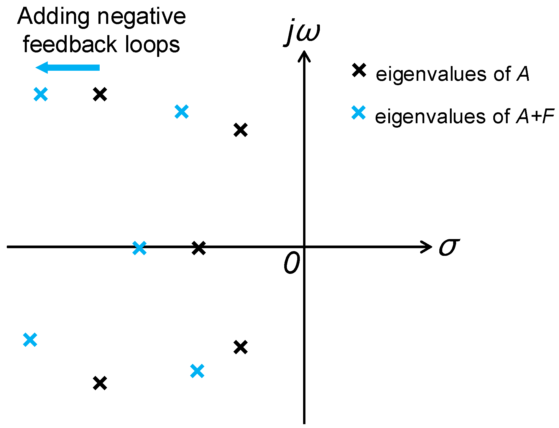
If the state feedback loops FX(t) with all eigenvalues in the left complex plane of the s-domain are developed for the stochastic biological network Equation (9) in the evolutionary process as follows:

$$\begin{array}{l}\dot{X}\left(t\right)=\left(A+{\displaystyle \sum _{i=1}^N{A}_i{n}_i\left(t\right)}\right)X\left(t\right)+FX\left(t\right)+Bv\left(t\right)\\ y\left(t\right)=CX\left(t\right)\end{array}$$

(15)

In this situation, the Riccati-like inequality in Equation (14) should be changed as:

$$C^{T}C+{\displaystyle \sum _{i=1}^N{A_i}^{T}P{A}_i+\frac{1}{r}PB{B}^{T}P\le -\left[P\left(A+F\right)+{\left(A+F\right)}^{T}P\right]}$$

(16)

Therefore, the biological network with feedback loops F to let all eigenvalues of A + F in the farther left complex plane of the s-domain will be with more stability robustness to tolerate more network random fluctuations and will decrease the network randomness and entropy to maintain its phenotype, i.e., a larger stability robustness in the right-hand side of Equation (16) will lead to less system randomness r or system entropy s tolerating larger random fluctuation term ${\displaystyle {\sum }_{i=1}^N{A_i}^{T}P{A}_i}$ due to ${\displaystyle {\sum }_{i=1}^N{A}_i{n}_i\left(t\right)}$ in Equation (15). However, if the added feedback loops F make the eigenvalues of A + F closer to the jω-axis than the eigenvalues of A, the feedback loops will increase the network randomness and entropy of the biological network.

(iv)

Dissipativity, all biological networks are open irreversible systems and the entropy production rate of biological system in Equation (16) is associated with the following dissipation rate η [26]:

$$\frac{E\left\{{\displaystyle {\int }_0^T{v}^T\left(t\right)y\left(t\right)dt}\right\}}{E\left\{{\displaystyle {\int }_0^T{v}^T\left(t\right)v\left(t\right)dt}\right\}}\le \eta ,\text{ for }X\left(0\right)=0,\eta \ge 0$$

By the following derivative procedure with V(X(t)) = X^T(t)PX(t) ≥ 0 and P > 0:

$$\begin{array}{l}E\left\{{\displaystyle {\int }_0^T{v}^T\left(t\right)y\left(t\right)dt}\right\}\\ =V\left(X(0)\right)-V\left(X(t)\right)+E\left\{{\displaystyle {\int }_0^T\left(v^T\left(t\right)y\left(t\right)+\frac{dV\left(X(t)\right)}{dt}\right)dt}\right\}\\ \le E\left\{{\displaystyle {\int }_0^T\left(v^T(t)y(t)+{\dot{X}}^T(t)PX(t)+X^T(t)P\dot{X}(t)+\frac{1}{2}{\displaystyle \sum _{i=1}^N{X}^T(t)A_i^T\frac{{\partial }^2{X}^T(t)PX(t)}{\partial X^2}{A}_{i}X(t)}\right)dt}\right\}\\ =\eta {\displaystyle {\int }_0^T{v}^T(t)v(t)}dt+{\displaystyle {\int }_0^T\left[\begin{array}{cc}{X}^T(t)& v^T(t)\end{array}\right]}\left[\begin{array}{cc}PA+A^{T}P+{\displaystyle \sum _{i=1}^N{A}_i^{T}P{A}_i}& PB+\frac{1}{2}{C}^T\\ B^{T}P+\frac{1}{2}C& -\eta I\end{array}\right]\left[\begin{array}{c}X(t)\\ v(t)\end{array}\right]\end{array}$$

If the following LMI holds:

$$\left[\begin{array}{cc}PA+A^{T}P+{\displaystyle \sum _{i=1}^N{A}_i^{T}P{A}_i}& PB+\frac{1}{2}{C}^T\\ B^{T}P+\frac{1}{2}C& -\eta I\end{array}\right]\le 0$$

we get $E\left\{{\displaystyle {\int }_0^T{v}^T(t)y(t)}\right\}\le \eta {\displaystyle {\int }_0^T{v}^T(t)v(t)}dt$ and the above LMI is equivalent to the following Riccati-like inequality:

$$PA+A^{T}P+{\displaystyle \sum _{i=1}^N{A}_i^{T}P{A}_i}+\eta \left(PB+\frac{1}{2}{C}^T\right)\left(B^{T}P+\frac{1}{2}C\right)\le 0$$

Comparing the above Ricatti-like inequality with Equation (14), there is an association with the system randomness r and the dissipation rate η.

2.2. On the Measurement of System Entropy in Nonlinear Stochastic Biological Network

In general, biological networks are always nonlinear. In this situation, the biological network in Equation (1) should be modified as the following nonlinear stochastic network:

$$\begin{array}{c}\dot{X}\left(t\right)=f\left(X\right)+g\left(X\right)v\left(t\right),X\left(0\right)=0\\ y\left(t\right)=h\left(X\right)\hfill \end{array}$$

(17)

where f(X) = [f₁(X) ... f_n(X)]^T denotes the nonlinear interactions among n species within the biological network, g(X) = [g₁(X) ... g_m(X)] denotes the nonlinear coupling between the biological network and the external input signal v(t). h(X) = [h₁(X) ... h_l(X)] denotes l nonlinear outputs.

Remark 5. The equilibrium point X_e of interest (i.e., the phenotype) of a nonlinear biological network is assumed at X(t) ≡ 0, i.e., X_e = 0. If the equilibrium point X_e ≠ 0, the origin of the nonlinear network must be shifted to X_e for the convenience of analysis. Similarly, the system entropy of the nonlinear biological network Equation (17) is defined as the logarithm of the system randomness in Equation (2). Based on the upper bound of the system randomness in Equation (3), we get the following result.

Proposition 3.

The system randomness of nonlinear stochastic network Equation (17) has an upper bound $\overline{r}$ if the following HJI has a positive Lyapunov solution V(X) > 0:

$${\left(\frac{\partial V\left(X\right)}{\partial X}\right)}^{T}f\left(X\right)+h^T\left(X\right)h\left(X\right)+\left(\frac{\partial V\left(X\right)}{\partial X}\right)g\left(X\right)v\left(t\right)-\overline{r}{v}^T\left(t\right)v\left(t\right)\le 0$$

(18)

Proof.

See Appendix C.

Since $\overline{r}$ is the upper bound of system randomness, from Proposition 3, the system randomness r of the nonlinear biological network in Equation (17) is calculated by solving the following HJI-constrained optimization:

$$r=\underset{V\left(X\right)>0}{\min }\overline{r}\mathrm{ subject\; to\; HJI\; in\; (18)}$$

(19)

After we solve the system randomness r from the HJI-constrained optimization problem Equation (19), the system entropy of the nonlinear biological network is obtained as s = log r.

Suppose the nonlinear biological network Equation (17) suffers from the following intrinsic random fluctuations due to N random noise sources n_i(t), for i = 1, ..., N:

$$\begin{array}{l}\dot{X}\left(t\right)=f\left(X\right)+{\displaystyle \sum _{i=1}^N{f}_i\left(X\right)}{n}_i\left(t\right)+g\left(X\right)v\left(t\right)\\ y\left(t\right)=h\left(X\right)\end{array}$$

(20)

where f_i(X) denotes the effect of the i-th random fluctuation source n_i(t) on the biological network.

The above nonlinear stochastic network can be represented by the following Itô stochastic process [57]:

$$\begin{array}{l}dX\left(t\right)=\left(f\left(X\right)+g\left(X\right)v\left(t\right)\right)dt+{\displaystyle \sum _{i=1}^N{f}_i\left(X\right)}d{w}_i\left(t\right)\\ y\left(t\right)=CX\left(t\right)\end{array}$$

(21)

where dw_i(t) = n_i(t) and w_i(t) denotes the Wiener process or Brownian motion. We then get the following result.

Proposition 4.

The system randomness of nonlinear stochastic network in Equation (20) with intrinsic random fluctuations has an upper bound $\overline{r}$ if the following HJI has a positive solution V(X) > 0:

$$\begin{array}{l}{\left(\frac{\partial V\left(X\right)}{\partial X}\right)}^{T}f\left(X\right)+h^T\left(X\right)h\left(X\right)+\left(\frac{\partial V\left(X\right)}{\partial X}\right)g\left(X\right)v\left(t\right)\\ +\frac{1}{2}{\displaystyle \sum _{i=1}^N{f_i}^T\left(X\right)}\frac{{\partial }^{2}V\left(X\right)}{\partial X^2}{f}_i\left(X\right)-\overline{r}{v}^T\left(t\right)v\left(t\right)\le 0\end{array}$$

(22)

Proof.

See Appendix D.

Therefore the following constrained optimization problem is required to solve and measure the system randomness in the nonlinear stochastic biological network in Equation (20):

$$r=\underset{V\left(X\right)>0}{\min }\overline{r}\mathrm{ subject\; to\; HJI\; in\; (22)}$$

(23)

After obtaining the HJI-constrained optimization in Equation (22) for system randomness r, the system entropy of nonlinear stochastic network Equation (20) can be obtained as s = log r.

Remark 6.

(i)

Comparing the HJI in Equation (18) with the HJI in Equation (22) when $\overline{r}$ is replaced by r, it is seen that the positive term ${\displaystyle {\sum }_{i=1}^N{f}_i^T\left(X\right)\left[{\partial }^{2}V\left(X\right)/\partial X^2\right]f_i\left(X\right)}$ in Equation (22) due to the random intrinsic fluctuations will cause a larger system randomness r and system entropy s for the nonlinear stochastic network in Equation (20).

(ii)

If some nonlinear feedback loops F(X) are developed for the nonlinear stochastic biological network Equation (20) in the evolutionary process as follows:

$$dX\left(t\right)=\left(f\left(X\right)+F\left(X\right)+g\left(X\right)v\left(t\right)\right)dt+{\displaystyle \sum _{i=1}^N{f}_i}\left(X\right)d{w}_i\left(t\right)$$

then the HJI in Equation (22) is modified as the following HJI:

$${\left(\frac{\partial V\left(X\right)}{\partial X}\right)}^T\left(f\left(X\right)+F\left(X\right)\right)+h^T\left(X\right)h\left(X\right)+{\left(\frac{\partial V\left(X\right)}{\partial X}\right)}^{T}g\left(X\right)v\left(t\right)+\frac{1}{2}{\displaystyle \sum _{i=1}^N{f_i}^T\left(X\right)\frac{{\partial }^{2}V\left(X\right)}{\partial X_2}}{f}_i\left(X\right)-\overline{r}{v}^T\left(t\right)v\left(t\right)\le 0$$

When comparing the above HJI with the HJI in (22), it is seen that the negative feedback loops F(X) will cause less system randomness and entropy while positive feedback loops can increase the system randomness and entropy of the nonlinear stochastic biological network.

In general, there is no efficient method to solve the HJI in Equations (18) or (22). Therefore, it is very difficult to solve the HJI-constrained optimization problem in Equations (19) or (23) for the entropy of the nonlinear biological network Equations (17) or the nonlinear stochastic biological network Equations (20). In order to solve the HJI-constrained optimization problems in Equations (19) and (23) for the calculation of the system randomness and entropy in nonlinear biological networks, the global linearization technique is employed in the following section to simplify the calculation procedure of system entropy.

2.3. The Calculation of System Entropy in Nonlinear Stochastic Biological Networks by the Global Linearization Method

In order to efficiently solve the HJI-constrained optimization problems in Equations (19) and (23) for the system randomness and entropy of nonlinear biological networks, the global linearization technique is employed to simplify the system-entropy measurement procedure by transforming the nonlinear biological network in Equations (17) to a set of interpolated local linearized linear biological networks.

By the global linearization method [26], if all the global linearizations are bounded by a polytope consisting of M vertices as [26,54,55,56]:

$$\left[\begin{array}{c}\frac{\partial f\left(X\right)}{\partial X}\\ \frac{\partial g\left(X\right)}{\partial X}\\ \frac{\partial h\left(X\right)}{\partial X}\end{array}\right]\in C_0\left(\begin{array}{ccccc}\left[\begin{array}{c}{A}_1\\ B_1\\ C_1\end{array}\right]& \cdots & \left[\begin{array}{c}{A}_i\\ B_i\\ C_i\end{array}\right]& \cdots & \left[\begin{array}{c}{A}_M\\ B_M\\ C_M\end{array}\right]\end{array}\right),\forall X\left(t\right)$$

(24)

where C₀ denotes the convex hull of polytope with M vertices defined in Equation (24), then the state trajectory X(t) of the nonlinear biological network (17) could be represented by the convex combination of the state trajectories of the following M local linearized biological networks derived from the vertices of the polytope in (24) [26,54,55,56]:

$$\begin{array}{l}\dot{X}\left(t\right)=A_{i}X\left(t\right)+B_{i}v\left(t\right),\text{ for }i=1,\cdots ,M\\ y\left(t\right)=C_{i}X\left(t\right)\end{array}$$

(25)

By the global linearization theory [26], if Equation (24) holds, then every trajectory of the nonlinear biological network in Equation (17) is a trajectory of a convex combination of M linearized biological networks in Equation (25). Therefore, if we can prove that the convex combination of M linearized biological networks in Equation (25) can represent the nonlinear biological network in Equation (17), then they will have the same system entropy. The convex combination of M linearized biological networks in Equation (25) can be represented as [58]:

$$\begin{array}{l}\dot{X}\left(t\right)={\displaystyle \sum _{i=1}^M{\alpha }_i}(X)\left(A_{i}X(t)+B_{i}v(t)\right)\\ y\left(t\right)={\displaystyle \sum _{i=1}^M{\alpha }_i}(X)C_{i}X(t)\end{array}$$

(26)

where the interpolation function ${\alpha }_i\left(X(t)\right)=\left(1/{\Vert X_i-X(t)\Vert }_2^2\right)/\left({\displaystyle {\sum }_{i=1}^M{\Vert X_i-X(t)\Vert }_2^2}\right)$ satisfies $0\le {\alpha }_i\left(X\right)\le 1$ and ${\displaystyle {\sum }_{i=1}^M{\alpha }_i\left(X\right)=1}$, i.e., the trajectories of the nonlinear biological network in Equation (17) can be represented by the interpolated biological networks in Equation (26), which is the convex combination of M local linearized biological networks at the vertices of polytope in Equation (25).

Remark 7. Actually, there are many interpolation methods to interpolate some local linearized networks at different operation points to approximate the nonlinear biological network in Equation (26), for example, interpolation methods by fuzzy bases [59,60] and cubic spline bases [61,62,63].

If the nonlinear biological network in Equation (17) could be approximated by the global linearization system in Equation (26), then based on Proposition 4 we get the following result.

Proposition 5.

The system randomness of the nonlinear stochastic network Equation (17) has an upper bound $\overline{r}$ if the following LMIs has a positive definite symmetry matrix P > 0:

$$\left[\begin{array}{cc}P{A}_i+{A_i}^{T}P+{C_i}^T{C}_i& P{B}_i\\ {B_i}^{T}P& -\overline{r}I\end{array}\right]\le 0,\text{ for }i=1,\cdots ,M$$

(27)

Proof.

See Appendix E.

Based on Schur complement [58], the LMIs in Equation (27) could be transformed to the following Riccati-like in equalities:

$$P{A}_i+{A_i}^{T}P+{C_i}^T{C}_i+\frac{1}{\overline{r}}P{B}_i{B_i}^{T}P\le 0,\text{ for }i=1,\cdots ,M$$

(28)

which is the same form as the Riccati-like equation in Equation (27) and can be considered as the local linearization set of HJI in Equation (18) at the M vertices of local linearized networks in Equation (17). Therefore, the system randomness $r$ of the nonlinear biological network Equation (17) or global linearization system Equation (26) can be calculated by solving the following LMIs-constrained optimization problem:

$$r=\underset{P>0}{\min }\overline{r}\mathrm{ subject\; to\; LMIs\; in\; (27)}$$

(29)

then the system entropy of the nonlinear biological network in Equations (17) or (26) can be obtained as s = log r. Substituting $r$ into $\overline{r}$ in Equations (28), we get:

$${C_i}^T{C}_i+\frac{1}{r}PB{B}^{T}P\le -\left(P{A}_i+{A_i}^{T}P\right)$$

(30)

Remark 8.

(i)

From Equation (30), it is seen that if the eigenvalues of local linearized system matrices A_i are all with more negative real part (more stable), then the nonlinear biological network in Equations (17) or (26) will be with less system randomness r and less system entropy s, and vice versa.

(ii)

The LMIs-constrained optimization problem for system randomness r in Equation (29) can be easily solved by decreasing $\overline{r}$ until no positive definite solution P > 0 exists in Equations (27) or (28) with the help of the LMI toolbox included in the Matlab software package.

After measuring the system randomness r and entropy s of the nonlinear biological network in Equation (17) by solving the LMIs-constrained optimization problem in Equation (29). We want to avoid solving the HJI-constrained optimization problem in Equation (23) to measure the system randomness and entropy of the nonlinear stochastic biological network (20) with intrinsic random fluctuations. Similarly, by following the global linearization of the nonlinear stochastic biological network Equation (20), if all the global linearized systems are bounded by a polytope consisting of the following M vertices [58]:

$$\left[\begin{array}{c}\frac{\partial f\left(X\right)}{\partial X}\\ \frac{\partial f_1\left(X\right)}{\partial X}\\ ⋮\\ \frac{\partial f_n\left(X\right)}{\partial X}\\ \frac{\partial g\left(X\right)}{\partial X}\\ \frac{\partial h\left(X\right)}{\partial X}\end{array}\right]\in C_0\left(\begin{array}{ccccc}\left[\begin{array}{c}{A}_1\\ A_{11}\\ ⋮\\ A_{1N}\\ B_1\\ C_1\end{array}\right]& \cdots & \left[\begin{array}{c}{A}_i\\ A_{i1}\\ ⋮\\ A_{iN}\\ B_i\\ C_i\end{array}\right]& \cdots & \left[\begin{array}{c}{A}_M\\ A_{M1}\\ ⋮\\ A_{MN}\\ B_M\\ C_M\end{array}\right]\end{array}\right),\forall X\left(t\right)$$

(31)

then the state trajectory X(t) of the nonlinear stochastic network in Equation (20) can be represented by the convex combination of the trajectories of the following M local linearized biological networks derived from the vertices of the polytope in Equation (31) [26,54,55,56]:

$$\begin{array}{l}\dot{X}\left(t\right)=A_{i}X\left(t\right)+{\displaystyle \sum _{j=1}^N{A}_{ij}X}\left(t\right)n_j\left(t\right)+B_{i}v\left(t\right),\text{ for }i=1,\cdots ,M\\ y\left(t\right)=C_{i}X\left(t\right)\end{array}$$

(32)

By the global linearization theory [26], if Equation (31) holds, then every trajectory of the nonlinear stochastic network in Equation (20) is a trajectory of a convex combination of M local linearized biological networks in Equation (32). Therefore, if we could prove that the convex combination of M linearized biological networks in Equation (32) can represent the nonlinear stochastic biological network in Equation (20), then they will have the same system randomness and entropy. The convex combination of M local linearized stochastic biological networks in Equation (32) can be represented as [26]:

$$\begin{array}{l}\dot{X}\left(t\right)={\displaystyle \sum _{i=1}^M{\alpha }_i\left(X\right)}\left(A_{i}X\left(t\right)+{\displaystyle \sum _{j=1}^N{A}_{ij}X\left(t\right)}{n}_j\left(t\right)+B_{i}v\left(t\right)\right)\\ y\left(t\right)={\displaystyle \sum _{i=1}^M{\alpha }_i\left(X\right)}{C}_{i}X\left(t\right)\end{array}$$

(33)

where the interpolation function ${\alpha }_i\left(X\right)$ satisfies $0\le {\alpha }_i\left(X\right)\le 1$ and ${\displaystyle {\sum }_{i=1}^M{\alpha }_i\left(X\right)}=1$, i.e., the interpolation of M local linearized stochastic biological networks in Equation (33) at M vertices in Equation (31) is employed to approach the nonlinear stochastic biological network in Equation (20).

After interpolating M local linear stochastic biological networks in Equation (33) to approximate the nonlinear biological network in Equation (20), we can get the following result.

Proposition 6.

If the following LMIs have a positive definite symmetry solution P > 0:

$$\left[\begin{array}{cc}P{A}_i+{A_i}^{T}P+{C_i}^T{C}_i+{\displaystyle \sum _{j=1}^N{A_{ij}}^{T}P}{A}_{ij}& P{B}_i\\ {B_i}^{T}P& -\overline{r}I\end{array}\right]\le 0,\text{ for }i=1,\cdots ,M$$

(34)

then the system randomness $r$ of the nonlinear stochastic biological network in Equations (20) or (33) has an upper bound $\overline{r}$.

Proof.

See Appendix F.

Remark 9. By Schur complement [26], the LMIs in Equation (34) are equivalent to the following Riccati-like inequalities:

$$P{A}_i+{A_i}^{T}P+{C_i}^T{C}_i+{\displaystyle \sum _{j=1}^N{A_{ij}}^{T}P{A}_{ij}+\frac{1}{\overline{r}}}P{B}_i{B_i}^{T}P\le 0,\text{ for }i=1,\cdots ,M$$

(35)

From the upper bound $\overline{r}$ of the system randomness in Equations (34) or (35), the system randomness of the nonlinear stochastic biological network in Equations (20) or (33) could be measured by solving the following LMIs-constrained minimization problem:

$$r=\underset{P>0}{\min }\overline{r}\mathrm{ subject\; to\; LMIs\; in\; (34)}$$

(36)

After solving the LMIs-constrained optimization in Equation (36) for the system randomness r of the nonlinear stochastic biological network in Equations (20) or (33), we could obtain the system entropy s = log r. If we substitute r for $\overline{r}$ in Equation (35), then we can get:

$${C_i}^T{C}_i+{\displaystyle \sum _{j=1}^N{A_{ij}}^{T}P{A}_{ij}+\frac{1}{\overline{r}}}P{B}_i{B_i}^{T}P\le -\left(P{A}_i+{A_i}^{T}P\right),\text{ for }i=1,\cdots ,M$$

(37)

From Equation (37), it is seen that the more negative eigenvalues of local system matrix A_i and the less local perturbations A_ij due to intrinsic random fluctuations will lead to a less system randomness r and system entropy s of the nonlinear stochastic biological network. If the eigenvalues of the biological system are fixed, large local perturbations A_ij may lead to large system randomness r. Larger input/output couplings B_i and C_i with environment will also lead to larger system randomness and entropy.

By multiplying Q = P⁻¹ > 0 to both sides of Equation (37) and r₁ = r⁻¹, we can get the following inequality:

$$A_{i}Q+Q{A_i}^T+Q{C_i}^T{C}_{i}Q+{\displaystyle \sum _{j=1}^{N}Q{A_{ij}}^T{Q}^{-1}{A}_{ij}Q+}{B}_i{\overline{r}}_1{B_i}^T\le 0$$

(38)

By Schur complement [26], Equation (38) is equivalent to:

$$\left[\begin{array}{ccccc}{A}_{i}Q+Q{A_i}^T+B{\overline{r}}_1{B}^T& Q^T{C_i}^T& Q{A_{i1}}^T& \cdots & Q{A_{iN}}^T\\ C_{i}Q& -1& 0& 0& 0\\ A_{i1}Q& 0& -Q& 0& 0\\ ⋮& 0& 0& -Q& 0\\ A_{iN}Q& 0& 0& 0& -Q\end{array}\right]<0$$

(39)

Therefore the minimization problem can be solved by the following expression:

$$r_1=\min {\overline{r}}_1\mathrm{ subject\; to\; LMIs\; into\; (39), }Q>0, r_1>0$$

(40)

system randomness r in Equation (36) can be resolved by r = r₁⁻¹ and P = Q⁻¹.

Remark 10.

(i)

Comparing Equation (30) with Equation (37), because of the positive term ${\displaystyle {\sum }_{j=1}^N{A_{ij}}^{T}P{A}_{ij}}$ due to intrinsic random fluctuations ${\displaystyle {\sum }_{j=1}^N{f}_i\left(x\right)n_i\left(t\right)}$ in the nonlinear stochastic biological network in Equation (20), system randomness r in Equation (37) must be larger than system randomness r in Equation (30) of the nonlinear biological network Equation (17) without intrinsic random fluctuations. Obviously, the intrinsic random fluctuations can increase system randomness r and system entropy s of the nonlinear biological networks.

(ii)

If the nonlinear stochastic biological network in Equation (20) has developed new feedback loops F(X) to tolerate network fluctuations as follows:

$$\dot{X}\left(t\right)=f\left(X\right)+F\left(X\right)+{\displaystyle \sum _{j=1}^N{f}_i\left(X\right)n_j\left(t\right)}+g\left(X\right)v\left(t\right)$$

(41)

which could be approximated by the following global linearization system:

$${\displaystyle \sum _{j=1}^N{A_{ij}}^{T}P{A}_{ij}+{C_i}^T{C}_i+\frac{1}{r}P{B}_i{B_i}^{T}P\le -\left[P\left(A_i+F_i\right)+{\left(A_i+F_i\right)}^{T}P\right]},\text{ for }i=1,\cdots ,M$$

(42)

where F(X) is approximated by ${\displaystyle {\sum }_{i=1}^M{\alpha }_i\left(X\right)F_{i}X\left(t\right)}$, then the Riccati-like inequality Equation (37) is replaced by Equation (39):

$${\displaystyle \sum _{j=1}^N{A_{ij}}^{T}P{A}_{ij}+{C_i}^T{C}_i+\frac{1}{r}P{B}_i{B_i}^{T}P\le -\left[P\left(A_i+F_i\right)+{\left(A_i+F_i\right)}^{T}P\right]},\text{ for }i=1,\cdots ,M$$

(43)

Obviously, feedback loops F(X) with the interpolation of M local feedback loops F_iX(t), for i = 1, ..., M, to shift all eigenvalues A_i + F_i to the farther left-hand plane of the s-domain will decrease the system randomness r and then decrease the entropy s of the nonlinear biological network in Equations (41) or (42) while the feedback loops F(X) with local F_iX(t), for i = 1, ..., M that makes the eigenvalues of A_i + F_i closer to the jω-axis will increase the system randomness and the entropy of the biological network in Equations (41) or (42).

Based on the above analysis, a measure procedure of system entropy for nonlinear biological networks is given as follows:

(i)

Construct nonlinear dynamic equations of biological networks as Equations (17) or (20).

(ii)

Use global linearization technique in Equations (24) or (31) to approximate the nonlinear biological network as Equations (26) or (33).

(iii)

Solve the LMIs-constrained optimization in Equations (29), (36) or (40) for the system randomness r and the entropy $s=\log r$ of the nonlinear biological network in Equations (17) or (20).

3. Example of Calculating System Entropy of Biological Networks

In this section two examples of calculating the system entropy of biological networks are given to illustrate the proposed system-entropy calculation methods; one example is about calculating the system entropy of a phosphorelay pathway in the molecular level and the other example is about calculating the system entropy of an ecological system.

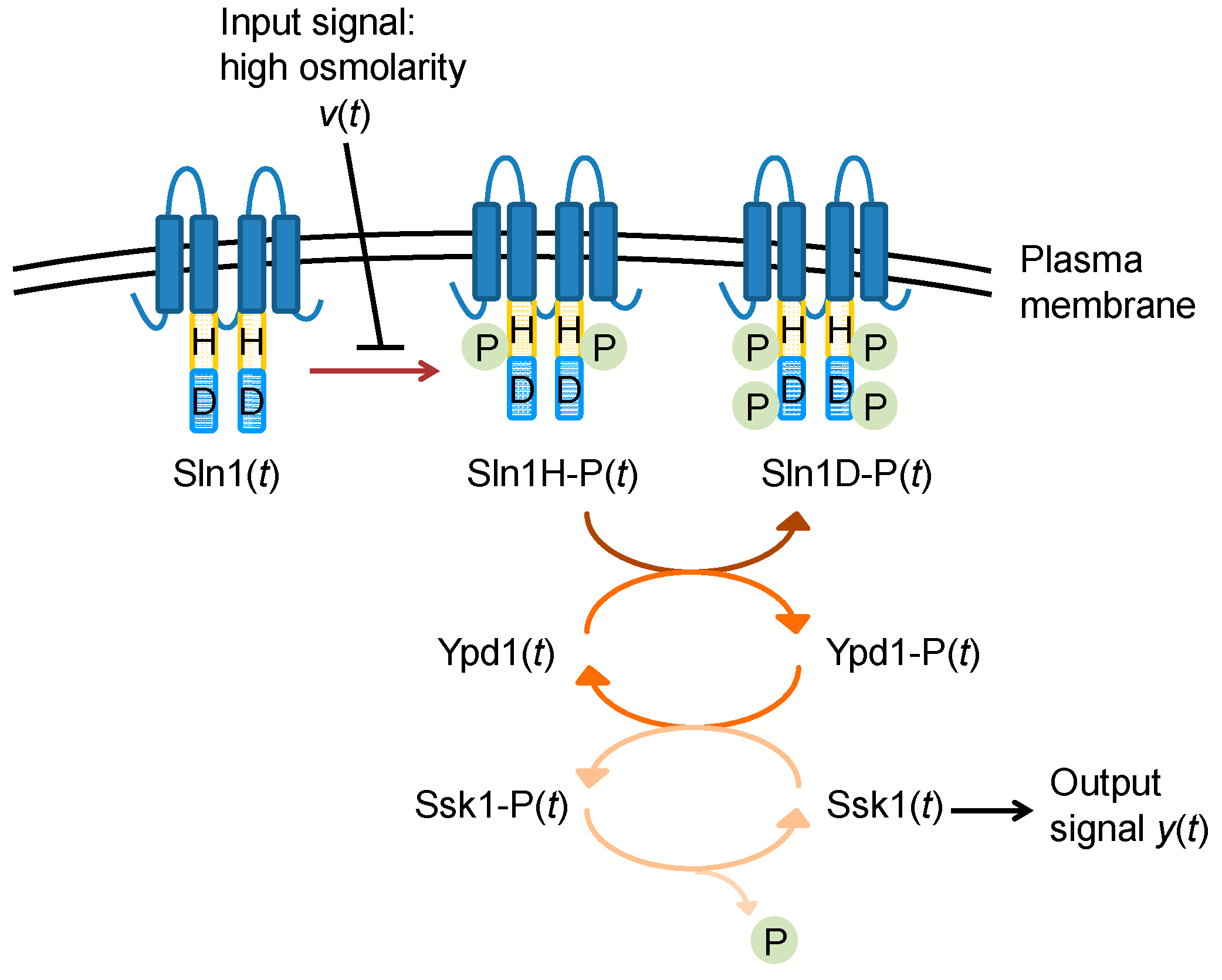
3.1. Example 1: The System Entropy of a Phosphorelay System

Consider a phosphorelay system from high osmolarity glycerol (HOG) signal pathway in yeast (Figure 3). This pathway is organized in the following [64]. It involves the transmembrane protein Sln1, which is present as a dimer. Under normal conditions, the signaling pathway is active due to continuous autophosphorylation at a histidine residue, Sln1H-P, under the consumption of ATP. Subsequently, this phosphate group is transferred to an aspartate group of Sln1 which is Sln1D-P, then to a histidine residue of Ypd1, and to an aspartate residue of Ssk1. Finally, Ssk1-P is continuously dephosphorylated by a phosphatase.

Figure 3. Schematic representation of phosphorelay system in example 1 consisting of Sln1-branch of high osmolarity glycerol (HOG) pathway in yeast [64].

Figure 3. Schematic representation of phosphorelay system in example 1 consisting of Sln1-branch of high osmolarity glycerol (HOG) pathway in yeast [64].

Let us denote X(t) = [x₁(t) x₂(t) x₃(t) x₄(t) x₅(t) x₆(t) x₇(t)]^T ≜ [Sln1(t) Sln1H-P(t) Sln1D-P(t) Ypd1(t) Ypd1-P(t) Ssk1(t) Ssk1-P(t)]^T. Then the dynamic behavior of the Sln1-phosphorelay system in yeast can be represented by the following dynamic equation [64]:

$$\begin{array}{l}{\dot{x}}_1\left(t\right)=-k_1{x}_1\left(t\right)+k_3{x}_3\left(t\right)x_4\left(t\right)+k_{0}v\left(t\right)\\ {\dot{x}}_2\left(t\right)=k_1{x}_1\left(t\right)-k_2{x}_2\left(t\right)\\ {\dot{x}}_3\left(t\right)=k_2{x}_2\left(t\right)-k_3{x}_3\left(t\right)x_4\left(t\right)\\ {\dot{x}}_4\left(t\right)=k_4{x}_5\left(t\right)x_6\left(t\right)-k_3{x}_3\left(t\right)x_4\left(t\right)\\ {\dot{x}}_5\left(t\right)=-k_4{x}_5\left(t\right)x_6\left(t\right)+k_3{x}_3\left(t\right)x_4\left(t\right)\\ {\dot{x}}_6\left(t\right)=k_5{x}_7\left(t\right)-x_4\left(t\right)x_5\left(t\right)x_6\left(t\right)\\ {\dot{x}}_7\left(t\right)=-k_5{x}_7\left(t\right)+x_4\left(t\right)x_5\left(t\right)x_6\left(t\right)\\ y=x_6\left(t\right)\end{array}$$

(44)

where k₀ = 0.5, k₁ = 0.4, k₂ = 0.1, k₃ = 50, k₄ = 50, k₅ = 0.5 and v(t) is white noise with zero mean and unit variance. The temporal profile of state variables of the Sln1-phosphorelay system is given in Figure 4a.

Figure 4. Temporal profiles of the state variables of Sln1-phosphorelay system (a) Sln1-phosphorelay system in Equation (44) and (b) Sln1-phosphorelay system with intrinsic random fluctuations in Equation (46). Both figures (a) and (b) were simulated by using Runge-Kutta scheme with the time step 0.01. The system entropy of (a) and (b) were measured as s = 3.5447 and s = 13.1483 by solving Equations (29) and (36), respectively. The overall system entropy increased when the intrinsic random fluctuations were considered.

Figure 4. Temporal profiles of the state variables of Sln1-phosphorelay system (a) Sln1-phosphorelay system in Equation (44) and (b) Sln1-phosphorelay system with intrinsic random fluctuations in Equation (46). Both figures (a) and (b) were simulated by using Runge-Kutta scheme with the time step 0.01. The system entropy of (a) and (b) were measured as s = 3.5447 and s = 13.1483 by solving Equations (29) and (36), respectively. The overall system entropy increased when the intrinsic random fluctuations were considered.

Based on the proposed measure procedure, we calculated the system entropy of the biological network. According to the global linearization in Equation (26), the Sln1-phosphorelay system in Equation (44) was represented by the following global linearization system:

$$\dot{X}\left(t\right)={\displaystyle \sum _{i=1}^4{\alpha }_i}(X)\left(A_{i}X(t)+B_{i}v(t)\right)$$

(45)

where the local linearized system matrices Ai, for i = 1, 2, 3, 4 are given in Appendix G. The interpolation functions are ${\alpha }_i\left(X(t)\right)=\left(1/{\Vert X_i-X(t)\Vert }_2^2\right)/\left({\displaystyle {\sum }_{i=1}^M{\Vert X_i-X(t)\Vert }_2^2}\right)$, where X(t) denotes the states of the proteins of the HOG system and X_i denotes the i-th local operation point with local linearization [33].

By solving the LMIs-constrained optimization problem in Equation (29) with:

$$P={10}^7\left[\begin{array}{ccccccc}0& 0& 0& 0& 0& 0& 0\\ 0& 0& 0& 0& 0& 0& 0\\ 0& 0& 0.0028& 0& 0.0005& 0.0005& -0.0051\\ 0& 0& 0& 0.1451& 0.1450& -0.0004& -0.0003\\ 0& 0& 0.0005& 0.1450& 0.1457& 0.0001& -0.0041\\ 0& 0& 0.0005& -0.0004& 0.0001& 2.1116& 2.0984\\ 0& 0& -0.0051& -0.0003& -0.0041& 2.0984& 2.2114\end{array}\right]$$

we measured the system randomness as r = 34.629 and the system entropy of the Sln1-phosphorelay system as s = 3.5447.

Suppose the Sln1-phosphorelay system suffered from the following two intrinsic random fluctuations from random noise sources n₁(t) and n₂(t):

$$\begin{array}{l}{\dot{x}}_1\left(t\right)=-k_1{x}_1\left(t\right)+k_3{x}_3\left(t\right)x_4\left(t\right)+0.1x_1\left(t\right)n_1\left(t\right)+k_{0}v\left(t\right)\\ {\dot{x}}_2\left(t\right)=k_1{x}_1\left(t\right)-k_2{x}_2\left(t\right)+0.2x_2\left(t\right)n_1\left(t\right)+0.1x_2\left(t\right)n_2\left(t\right)\\ {\dot{x}}_3\left(t\right)=k_2{x}_2\left(t\right)-k_3{x}_3\left(t\right)x_4\left(t\right)+0.1x_2\left(t\right)x_4\left(t\right)n_1\left(t\right)\\ {\dot{x}}_4\left(t\right)=k_4{x}_5\left(t\right)x_6\left(t\right)-k_3{x}_3\left(t\right)x_4\left(t\right)+0.1x_5\left(t\right)x_6\left(t\right)n_2\left(t\right)+0.1x_3\left(t\right)x_4\left(t\right)n_1\left(t\right)\\ {\dot{x}}_5\left(t\right)=-k_4{x}_5\left(t\right)x_6\left(t\right)+k_3{x}_3\left(t\right)x_4\left(t\right)+0.2x_5\left(t\right)x_6\left(t\right)n_2\left(t\right)+0.2x_3\left(t\right)x_4\left(t\right)n_1\left(t\right)\\ {\dot{x}}_6\left(t\right)=k_5{x}_7\left(t\right)-x_4\left(t\right)x_5\left(t\right)x_6\left(t\right)+0.1x_7\left(t\right)n_1\left(t\right)+0.1x_5\left(t\right)x_6\left(t\right)n_2\left(t\right)\\ {\dot{x}}_7\left(t\right)=-k_5{x}_7\left(t\right)+x_4\left(t\right)x_5\left(t\right)x_6\left(t\right)+0.1x_7\left(t\right)n_1\left(t\right)+0.1x_5\left(t\right)x_6\left(t\right)n_2\left(t\right)\\ y=x_6\left(t\right)\end{array}$$

(46)

where n₁(t) and n₂(t) were independent white noise with zero mean and unit variance. The temporal profile of the stochastic biological network Equation (46) with intrinsic random fluctuations is given in Figure 4b. From Equation (33), the nonlinear stochastic biological network in Equation (46) was approximated by the following global linearization system:

$$\dot{X}\left(t\right)={\displaystyle \sum _{i=1}^4{\alpha }_i}\left(X\right)\left(A_{i}X\left(t\right)+{\displaystyle \sum _{j=1}^2{A}_{ij}X\left(t\right)n_j}+B_{i}v\left(t\right)\right)$$

(47)

where A_i is the same as Equation (45) and A_ij, for i = 1,2,3,4, j = 1, 2 are also given in Appendix G. By solving the LMIs-constrained optimization problem in Equation (36) with:

$$P={10}^4\left[\begin{array}{ccccccc}0.3275& 0.3432& 0.3263& 0.0082& 0.0077& 0.0232& 0.0182\\ 0.3432& 0.3729& 0.3416& 0.0057& 0.0053& 0.0379& 0.0110\\ 0.3263& 0.3416& 0.3325& -0.0039& 0.0024& 0.0627& 0.0125\\ 0.0082& 0.0057& -0.0039& 0.6919& 0.6803& -2.3615& -2.0463\\ 0.0077& 0.0053& 0.0024& 0.06803& 0.6762& -2.3233& -2.0498\\ 0.0232& 0.0379& 0.0627& -2.3615& -2.3233& 8.5551& 7.3236\\ 0.0182& 0.0110& 0.0125& -2.0463& -2.0498& 7.3236& 7.8763\end{array}\right]$$

We measured the system randomness as r = 5.1314 × 10⁵ and the system entropy of the nonlinear stochastic biological network Equation (46) as s = 13.1483, which were much larger than the system randomness and system entropy of biological network without intrinsic random fluctuations in Equation (44). Obviously, the intrinsic random fluctuations in Equation (46) will increase the system entropy of the biological network.

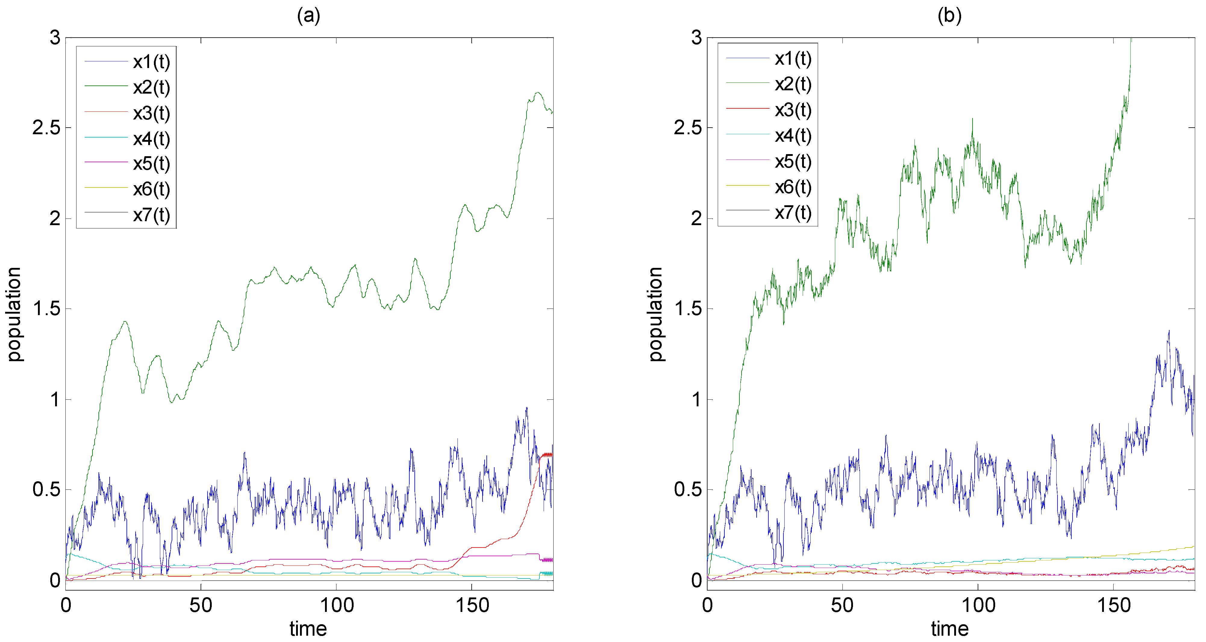
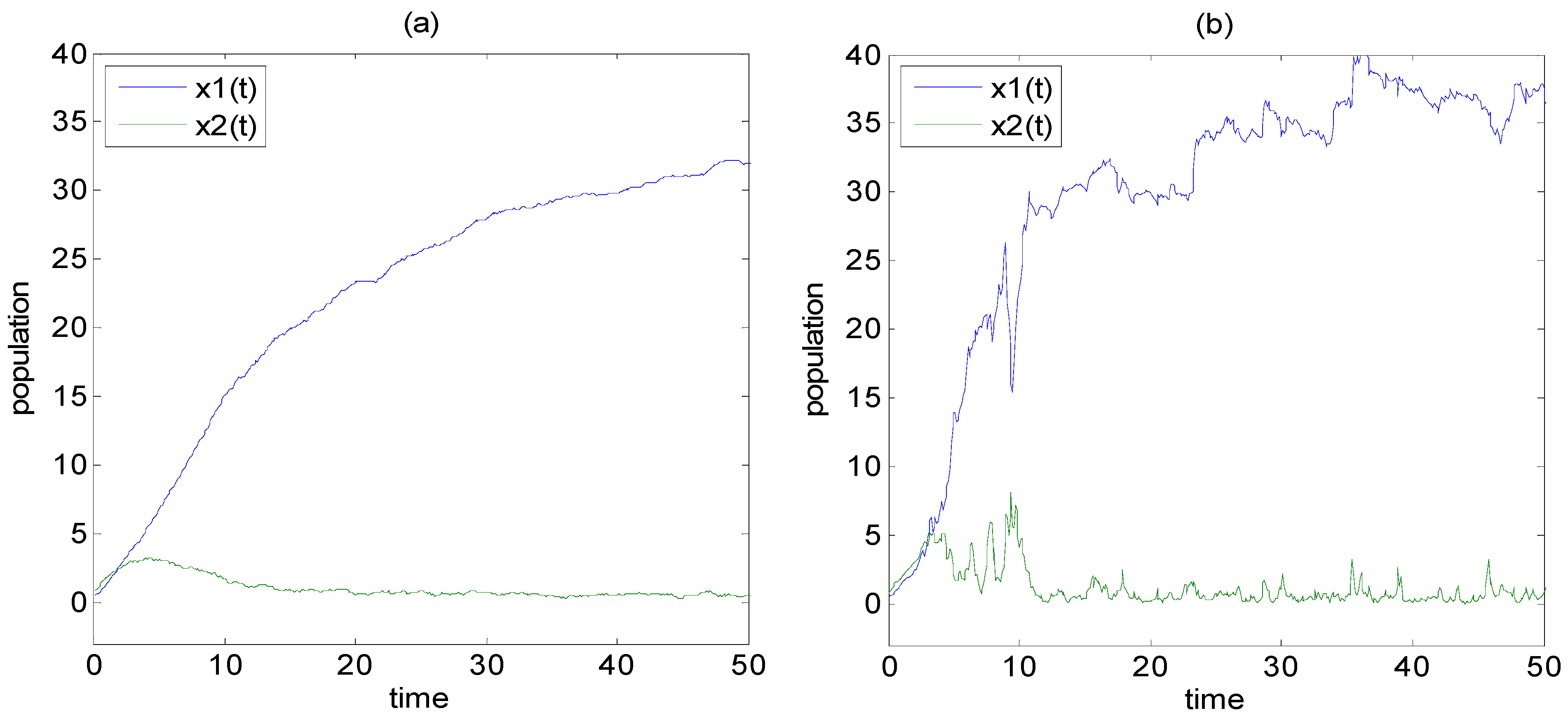
3.2. Example 2: The System Entropy of Predator-Prey Ecological System

Consider the following predator-prey ecological system [65]:

$$\begin{array}{l}{\dot{x}}_1\left(t\right)=-0.05x_1\left(t\right)+0.05x_1\left(t\right)x_2\left(t\right)+h_1{v}_1\left(t\right)\\ {\dot{x}}_2\left(t\right)=0.05x_2\left(t\right)-0.06x_1\left(t\right)x_2\left(t\right)+h_2{v}_2\left(t\right)\\ y\left(t\right)=\left[\begin{array}{c}{x}_1\left(t\right)\\ x_2\left(t\right)\end{array}\right]\end{array}$$

(48)

where h₁ = 0.8, h₂ = 0.8 and v₁(t), v₂(t) are the external inputs with zero mean unit variance white noise. The simulation of the predator-prey ecological system in Equation (48) is shown in Figure 5a. Based on global linearization in Equation (26), the predator-prey ecological system in Equation (48) can be approximated by the following global linearization system:

$$\dot{X}\left(t\right)={\displaystyle \sum _{i=1}^4{\alpha }_i}(X)\left(A_{i}X(t)+B_{i}v(t)\right)$$

(49)

where the interpolation functions are ${\alpha }_i\left(X(t)\right)=\left(1/{\Vert X_i-X(t)\Vert }_2^2\right)/\left({\displaystyle {\sum }_{i=1}^M{\Vert X_i-X(t)\Vert }_2^2}\right)$, where X(t) denotes the states of the population of the prey or predator system and X_i denotes the i-th local operation point with local linearization [33]. The local linearized system matrices A_i, for i = 1,2,3,4 are given in Appendix H. The temporal profile of the predator and prey population in Equation (48) is shown in Figure 5a.

By solving the LMIs-constrained optimization in Equation (29), the measurement of the system randomness and entropy with $P=\left[\begin{array}{cc}1.7498& 0\\ 0& 1.7618\end{array}\right]$ was acquired as follows: system randomness $r$ = 14.73831 and the system entropy s = 2.6905.

Suppose the predator-prey system suffered from the following intrinsic random fluctuations from two random noise sources n₁(t) and n₂(t):

$$\begin{array}{l}{\dot{x}}_1\left(t\right)=-0.05x_1\left(t\right)+0.05x_1\left(t\right)x_2\left(t\right)+0.2x_1\left(t\right)x_2\left(t\right)n_1\left(t\right)+h_1{v}_1\left(t\right)\\ {\dot{x}}_2\left(t\right)=0.05x_2\left(t\right)-0.06x_1\left(t\right)x_2\left(t\right)-0.2x_1\left(t\right)x_2\left(t\right)n_2\left(t\right)+h_2{v}_2\left(t\right)\\ y\left(t\right)=\left[\begin{array}{c}{x}_1\left(t\right)\\ x_2\left(t\right)\end{array}\right]\end{array}$$

(50)

where h₁ = 0.8, h₂ = 0.8 and n₁(t), n₂(t) are independent white noise with zero mean and unit variance.

From Equation (33), the nonlinear stochastic predator-prey system in Equation (50) was approximated by the following global linearization system:

$$\dot{X}\left(t\right)={\displaystyle \sum _{i=1}^4{\alpha }_i}\left(X\right)\left(A_{i}X\left(t\right)+{\displaystyle \sum _{j=1}^2{A}_{ij}X\left(t\right)n_j}+B_{i}v\left(t\right)\right)$$

(51)

where A_i is the same as Equation (49) and A_ij, for i = 1,2,3,4, j = 1,2 are also given in Appendix H. The temporal profile of the predator and prey population with intrinsic random fluctuations is shown in Figure 5(b). By solving the LMIs-constrained optimization problem in Equation (40) with $P=\left[\begin{array}{cc}0.2946& 0.0527\\ 0.0527& 0.2070\end{array}\right]$, the system randomness was measured as r = 26.0657 and the system entropy of nonlinear stochastic network in Equation (50) was measured as s = 3.2606, which were larger than the system entropy of biological network without intrinsic random fluctuations in Equation (48). Obviously, the intrinsic random fluctuations will increase the system entropy of the ecological network.

Figure 5. Simulation of the gowth and decline of (a) the predator-prey system in Equation (48) and (b) the predator-prey system with intrinsic random fluctuations in Equation (50). Both figures (a) and (b) were simulated by using Runge-Kutta scheme with the time step 0.01. The system entropy of (a) and (b) were measured as s = 2.6905 and s = 3.2606 by solving Equations (29) and (40), respectively. The overall system entropy increased when the intrinsic random fluctuations were considered.

Figure 5. Simulation of the gowth and decline of (a) the predator-prey system in Equation (48) and (b) the predator-prey system with intrinsic random fluctuations in Equation (50). Both figures (a) and (b) were simulated by using Runge-Kutta scheme with the time step 0.01. The system entropy of (a) and (b) were measured as s = 2.6905 and s = 3.2606 by solving Equations (29) and (40), respectively. The overall system entropy increased when the intrinsic random fluctuations were considered.

4. Conclusions

Based on the difference between input signal entropy and output signal entropy, a determination of the system entropy of a nonlinear stochastic biological network was introduced for the first time in this study. An indirect method was also proposed to measure system entropy by minimizing its upper bound. We found that system entropy of biological systems is determined by their system matrices and parameter fluctuations. A global linearization scheme was employed to avoid the necessity for solving a difficult HJI-constrained optimization problem to measure the system entropy of nonlinear stochastic biological networks. This scheme replaces the HJI-constrained optimization problem with a LMIs-constrained optimization problem, which can be efficiently solved using the LMI toolbox provided by the Matlab software. We found that the system entropy of biological networks is inversely proportional to their robustness and stability, and that intrinsic random fluctuations can increase the system entropy. We also found that a feedback loop that could shift all eigenvalues to the farther left-hand plane of s-domain decreases the system entropy, while a feedback loop that makes the eigenvalues of A + F closer to the jω-axis than the eigenvalues of A increases the system entropy. Redundancy can attenuate the intrinsic random fluctuations due to genetic mutations and epigenetic alterations, and therefore, decrease the system entropy of a biological network. Furthermore, the proposed system entropy calculation method for nonlinear stochastic biological networks can applied to the estimation of the influence on the system entropy by feedback loops added to the biological system in the field of synthetic biology or metabolic flux analysis in metabolomics, etc. From our measurements of the system entropy of biological networks, we were able to gain a greater, more systematic insight into the behavior of living systems.

References

1. Mettetal, J.T.; van Oudenaarden, A. Microbiology. Necessary noise. Science 2007, 317, 463–464. [Google Scholar] [CrossRef] [PubMed]
2. Pedraza, J.M.; van Oudenaarden, A. Noise propagation in gene networks. Science 2005, 307, 1965–1969. [Google Scholar] [CrossRef] [PubMed]
3. Mettetal, J.T.; Muzzey, D.; Pedraza, J.M.; Ozbudak, E.M.; van Oudenaarden, A. Predicting stochastic gene expression dynamics in single cells. Proc. Natl. Acad. Sci. USA 2006, 103, 7304–7309. [Google Scholar] [CrossRef] [PubMed]
4. Krawitz, P.; Shmulevich, I. Basin Entropy in Boolean Network Ensembles. Phys. Rev. Lett. 2007, 98, 158701. [Google Scholar] [CrossRef] [PubMed]
5. Krawitz, P.; Shmulevich, I. Entropy of complex relevant components of Boolean networks. Phys. Rev. E 2007, 76, 036115. [Google Scholar] [CrossRef]
6. Johansson, R. System Modeling and Identification; Springer: London, UK, 1993. [Google Scholar]
7. Demetrius, L. Thermodynamics and evolution. J. Theor. Biol. 2000, 206, 1–16. [Google Scholar] [CrossRef] [PubMed]
8. Chen, B.-S.; Li, C.-W. On the Interplay between Entropy and Robustness of Gene Regulatory Networks. Entropy 2010, 12, 1071–1101. [Google Scholar] [CrossRef]
9. Schrödinger, E. What is Life? 1944. Available online: http://159.226.251.229/videoplayer/What-is-Life.pdf?ich_u_r_i=79fe139669467dd24cdc11542b4e002f&ich_s_t_a_r_t=0&ich_e_n_d=0&ich_k_e_y=1545108906750663172441&ich_t_y_p_e=1&ich_d_i_s_k_i_d=3&ich_u_n_i_t=1 (accessed on 6 October 2015).
10. Lucia, U. Irreversible entropy variation and the problem of the trend to equilibrium. Phys. A 2007, 376, 289–292. [Google Scholar] [CrossRef]
11. Lucia, U. Irreversibility, entropy and incomplete information. Phys. A 2009, 388, 4025–4033. [Google Scholar] [CrossRef]
12. Lucia, U. Maximum entropy generation and kappa-exponential model. Phys. A 2010, 389, 4558–4563. [Google Scholar] [CrossRef]
13. Lucia, U. The Gouy-Stodola Theorem in Bioenergetic Analysis of Living Systems (Irreversibility in Bioenergetics of Living Systems). Energies 2014, 7, 5717–5739. [Google Scholar] [CrossRef]
14. Lucia, U.; Ponzetto, A.; Deisboeck, T.S. A thermodynamic approach to the ‘mitosis/apoptosis’ ratio in cancer. Phys. A 2015, 436, 246–255. [Google Scholar] [CrossRef]
15. Boyd, S.P.; Barratt, C.H.; Boyd, S.P.; Boyd, S.P. Linear Controller Design: Limits of Performance; Prentice-Hall: Upper Saddle River, NJ, USA, 1991. [Google Scholar]
16. Chen, B.-S.; Chang, Y.-T.; Wang, Y.-C. Robust H∞ stabilization design in gene networks under stochastic molecular noises: Fuzzy-interpolation approach. IEEE Trans. Syst. Man Cybern B Cybern. 2008, 38, 25–42. [Google Scholar] [CrossRef] [PubMed]
17. Díaz, J.; Alvarez-Buylla, E.R. Information flow during gene activation by signaling molecules: Ethylene transduction in Arabidopsis cells as a study system. BMC Syst. Biol. 2009, 3. [Google Scholar] [CrossRef] [PubMed]
18. Lezon, T.R.; Banavar, J.R.; Cieplak, M.; Maritan, A.; Fedoroff, N.V. Using the principle of entropy maximization to infer genetic interaction networks from gene expression patterns. Proc. Natl. Acad. Sci. USA 2006, 103, 19033–19038. [Google Scholar] [CrossRef] [PubMed]
19. Manke, T.; Demetrius, L.; Vingron, M. An entropic characterization of protein interaction networks and cellular robustness. J. R. Soc. Interface 2006, 3, 843–850. [Google Scholar] [CrossRef]
20. McAdams, H.H.; Arkin, A. It’s a noisy business! Genetic regulation at the nanomolar scale. Trends Genet. 1999, 15, 65–69. [Google Scholar] [CrossRef]
21. Nagarajan, R.; Aubin, J.E.; Peterson, C.A. Robust dependencies and structures in stem cell differentiation. Int. J. Bifurc. Chaos 2005, 15, 1503–1514. [Google Scholar] [CrossRef]
22. Stoll, G.; Rougemont, J.; Naef, F. Representing perturbed dynamics in biological network models. Phys. Rev. E Stat. Nonlin. Soft Matter. Phys. 2007, 76, 011917. [Google Scholar] [CrossRef] [PubMed]
23. Wang, X.-L.; Yuan, Z.-F.; Guo, M.-C.; Song, S.-D.; Zhang, Q.-Q.; Bao, Z. Maximum entropy principle and population genetic equilibrium. Acta. Genet. Sin. 2002, 29, 562–564. [Google Scholar] [PubMed]
24. Wlaschin, A.P.; Trinh, C.T.; Carlson, R.; Srienc, F. The fractional contributions of elementary modes to the metabolism of Escherichia coli and their estimation from reaction entropies. Metab. Eng. 2006, 8, 338–352. [Google Scholar] [CrossRef] [PubMed]
25. Yildirim, N.; Mackey, M.C. Feedback regulation in the lactose operon: A mathematical modeling study and comparison with experimental data. Biophys. J. 2003, 84, 2841–2851. [Google Scholar] [CrossRef]
26. Boyd, S.P.; El Ghaoui, L.; Feron, E.; Balakrishnan, V. Linear Matrix Inequalities in System and Control Theory; SIAM: Philadelphia, PA, USA, 1994. [Google Scholar]
27. Kitano, H. Biological robustness. Nat. Rev. Genet. 2004, 5, 826–837. [Google Scholar] [CrossRef] [PubMed]
28. Wang, J.; Xu, L.; Wang, E. Potential landscape and flux framework of nonequilibrium networks: Robustness, dissipation, and coherence of biochemical oscillations. Proc. Natl. Acad. Sci. USA 2008, 105, 12271–12276. [Google Scholar] [CrossRef] [PubMed]
29. Krantz, M.; Ahmadpour, D.; Ottosson, L.G.; Warringer, J.; Waltermann, C.; Nordlander, B.; Klipp, E.; Blomberg, A.; Hohmann, S.; Kitano, H. Robustness and fragility in the yeast high osmolarity glycerol (HOG) signal-transduction pathway. Mol. Syst. Biol. 2009, 5. [Google Scholar] [CrossRef] [PubMed]
30. Lenz, P.; Swain, P.S. An entropic mechanism to generate highly cooperative and specific binding from protein phosphorylations. Curr. Biol. 2006, 16, 2150–2155. [Google Scholar] [CrossRef] [PubMed]
31. Chen, B.-S.; Chang, Y.-T. A systematic molecular circuit design method for gene networks under biochemical time delays and molecular noises. BMC Syst. Biol. 2008, 2. [Google Scholar] [CrossRef] [PubMed]
32. Chen, B.S.; Chen, P.W. Robust Engineered Circuit Design Principles for Stochastic Biochemical Networks With Parameter Uncertainties and Disturbances. IEEE Trans. Biomed. Circuits Syst. 2008, 2, 114–132. [Google Scholar] [CrossRef] [PubMed]
33. Chen, B.-S.; Chen, P.-W. On the estimation of robustness and filtering ability of dynamic biochemical networks under process delays, internal parametric perturbations and external disturbances. Math. Biosci. 2009, 222, 92–108. [Google Scholar] [CrossRef] [PubMed]
34. Hasty, J.; McMillen, D.; Collins, J.J. Engineered gene circuits. Nature 2002, 420, 224–230. [Google Scholar] [CrossRef] [PubMed]
35. Lapidus, S.; Han, B.; Wang, J. Intrinsic noise, dissipation cost, and robustness of cellular networks: The underlying energy landscape of MAPK signal transduction. Proc. Natl. Acad. Sci. USA 2008, 105, 6039–6044. [Google Scholar] [CrossRef] [PubMed]
36. Batt, G.; Yordanov, B.; Weiss, R.; Belta, C. Robustness analysis and tuning of synthetic gene networks. Bioinformatics 2007, 23, 2415–2422. [Google Scholar] [CrossRef] [PubMed]
37. Kærn, M.; Elston, T.C.; Blake, W.J.; Collins, J.J. Stochasticity in gene expression: From theories to phenotypes. Nat. Rev. Genet. 2005, 6, 451–464. [Google Scholar] [CrossRef] [PubMed]
38. Voit, E.O. Computational Analysis of Biochemical Systems: A Practical Guide for Biochemists and Molecular Biologists; Cambridge University Press: Cambridge, UK, 2000. [Google Scholar]
39. Chen, B.S.; Li, C.W. On the noise enhancing of stochastic Hodgkin-Hurley neuron systems. Neural Comput. 2012, 22, 1737–1763. [Google Scholar] [CrossRef] [PubMed]
40. Chen, B.S.; Wu, W.S.; Wang, Y.C.; Li, W.H. On the Robust Circuit Design Schemes of Biochemical Networks: Steady-State Approach. IEEE Trans. Biomed. Circuits Syst. 2007, 1, 91–104. [Google Scholar] [CrossRef] [PubMed]
41. Chen, B.S.; Li, C.-W. Stochastic Spatio-Temporal Dynamic Model for Gene/Protein Interaction Network in Early Drosophila Development. Gene Regul Syst. Biol. 2009, 3, 191–210. [Google Scholar]
42. Chen, B.S.; Wu, W.S. Underlying Principles of Natural Selection in Network Evolution: Systems Biology Approach. Evol. Bioinfom. 2007, 3, 245–262. [Google Scholar]
43. Chen, B.S.; Wu, W.S.; Wu, W.S.; Li, W.H. On the Adaptive Design Rules of Biochemical Networks in Evolution. Evol. Bioinfom. 2007, 3, 27–39. [Google Scholar]
44. Chen, B.S.; Ho, S.J. The stochastic evolutionary game for a population of biological networks under natural selection. Evol. Bioinform. Online 2014, 10, 17–38. [Google Scholar] [CrossRef] [PubMed]
45. Chen, B.S.; Zhang, W.H. Stochastic H2/H∞ Control With State-Dependent Noise. IEEE Trans. Auto. Cont. 2004, 49, 45–57. [Google Scholar] [CrossRef]
46. Blake, W.J.; Kærn, M.; Cantor, C.R.; Collins, J.J. Noise in eukaryotic gene expression. Nature 2003, 422, 633–637. [Google Scholar] [CrossRef] [PubMed]
47. Arkin, A.; McAdams, H.H. Stochastic mechanisms in gene expression. Proc. Natl. Acad. Sci. USA 1997, 94, 814–819. [Google Scholar]
48. Freeman, S.; Herron, J.C. Evolutionary Analysis, 3rd ed; Pearson Prentice Hall: Upper Saddle River, NJ, USA, 2004. [Google Scholar]
49. Freeman, M. Feedback control of intercellular signalling in development. Nature 2000, 408, 313–319. [Google Scholar] [CrossRef] [PubMed]
50. Lynch, M.; Walsh, B. Genetics and Analysis of Quantitative Traits, 1st ed.; Sinauer Associates: Sunderland, MA, USA, 1998. [Google Scholar]
51. Chen, B.-S.; Lin, Y.-P. On the Interplay between the Evolvability and Network Robustness in an Evolutionary Biological Network: A Systems Biology Approach. Evol. Bioinform. Online 2011, 7, 201–233. [Google Scholar] [CrossRef] [PubMed]
52. Popkov, Y.; Popkov, A. New Methods of Entropy-Robust Estimation for Randomized Models under Limited Data. Entropy 2014, 16, 675–698. [Google Scholar] [CrossRef]
53. Mall, R.; Langone, R.; Suykens, J.A. Kernel Spectral Clustering for Big Data Networks. Entropy 2013, 15, 1567–1586. [Google Scholar] [CrossRef]
54. Chen, B.-S.; Wang, Y.-C. On the attenuation and amplification of molecular noise in genetic regulatory networks. BMC Bioinform. 2006, 7. [Google Scholar] [CrossRef]
55. Chen, B.-S.; Wang, Y.-C.; Wu, W.-S.; Li, W.-H. A new measure of the robustness of biochemical networks. Bioinformatics 2005, 21, 2698–2705. [Google Scholar] [CrossRef] [PubMed]
56. Chen, B.-S.; Wu, W.-S. Robust filtering circuit design for stochastic gene networks under intrinsic and extrinsic molecular noises. Math. Biosci. 2008, 211, 342–355. [Google Scholar] [CrossRef] [PubMed]
57. Zhang, W.; Chen, B.-S. State Feedback H∞ Control for a Class of Nonlinear Stochastic Systems. SIAM J. Control Optim. 2006, 44, 1973–1991. [Google Scholar] [CrossRef]
58. Zhang, W.; Chen, B.-S. On stabilizability and exact observability of stochastic systems with their applications. Automatica 2004, 40, 87–94. [Google Scholar] [CrossRef]
59. Chen, B.-S.; Tseng, C.-S.; Uang, H.-J. Robustness Design of Nonlinear Dynamic Systems via Fuzzy Linear Control. IEEE Fuzzy Syst. 1999, 7, 571–585. [Google Scholar] [CrossRef]
60. Chen, B.-S.; Tseng, C.-S.; Uang, H.-J. Mixed H2/H∞ Fuzzy Output Feedback Control Design for Nonlinear Dynamic Systems: An LMI Approach. IEEE Trans. Fuzzy Syst. 2000, 8, 249–265. [Google Scholar] [CrossRef]
61. Chen, B.-S.; Lin, Y.-P. A Unifying Mathematical Framework for Genetic Robustness, Environmental Robustness, Network Robustness and their Trade-off on Phenotype Robustness in Biological Networks Part I: Gene Regulatory Networks in Systems and Evolutionary Biology. Evol. Bioinform. Online 2013, 9, 43–68. [Google Scholar] [CrossRef] [PubMed]
62. Chen, B.-S.; Lin, Y.-P. A Unifying Mathematical Framework for Genetic Robustness, Environmental Robustness, Network Robustness and their Trade-offs on Phenotype Robustness in Biological Networks. Part II: Ecological networks. Evol. Bioinform. Online 2013, 9, 69–85. [Google Scholar] [CrossRef] [PubMed]
63. Chen, B.-S.; Lin, Y.-P. A Unifying Mathematical Framework for Genetic Robustness, Environmental Robustness, Network Robustness and their Trade-offs on Phenotype Robustness in Biological Networks. Part III: Synthetic Gene Networks in Synthetic Biology. Evol. Bioinform. Online 2013, 9, 87–109. [Google Scholar] [CrossRef] [PubMed]
64. Klipp, E.; Herwig, R.; Kowald, A.; Wierling, C.; Lehrach, H. Systems Biology in Practice: Concepts, Implementation and Applcation; Wiley: New York, NY, USA, 2005. [Google Scholar]
65. Murray, J.D. Mathematical Biology, 3rd ed; Springer: Berlin/Heidelberg, Germany, 2003. [Google Scholar]
66. Zhang, W.; Chen, B.-S.; Tseng, C.-S. Robust H∞ Filtering for Nonlinear Stochastic Systems. IEEE Trans. Sig. Process 2005, 53, 589–598. [Google Scholar] [CrossRef]
67. Zhang, W.; Zhang, H.; Chen, B.-S. Stochastic H2/H∞ control with (x, u, v)-dependent noise: Finite horizon case. Automatica 2006, 42, 1891–1898. [Google Scholar] [CrossRef]
68. Zhang, W.; Chen, B.-S. H-Representation and Applications to Generalized Lyapunov Equations and Linear Stochastic Systems. IEEE Trans. Auto. Cont. 2012, 57, 3009–3022. [Google Scholar] [CrossRef]
69. Zhang, W.; Chen, B.-S.; Sheng, L.; Gao, M. Robust H2/H∞ Filter Design for a Class of Nonlinear Stochastic Systems with State-Dependent Noise. Math. Probl. Eng. 2012, 2012, 1–16. [Google Scholar]