Comparison of Vegetation Indices for Leaf Area Index Estimation in Vertical Shoot Positioned Vine Canopies with and without Grenbiule Hail-Protection Netting

Abstract

Leaf area per unit surface (LAI—leaf area index) is a valuable parameter to assess vine vigour in several applications, including direct mapping of vegetative–reproductive balance (VRB). Normalized difference vegetation index (NDVI) has been successfully used to assess the spatial variability of estimated LAI. However, sometimes NDVI is unsuitable due to its lack of sensitivity at high LAI values. Moreover, the presence of hail protection with Grenbiule netting also affects incident light and reflection, and consequently spectral response. This study analyses the effect of protective netting in the LAI–NDVI relationship and, using NDVI as a reference index, compares several indices in terms of accuracy and sensitivity using linear and logarithmic models. Among the indices compared, results show NDVI to be the most accurate, and ratio vegetation index (RVI) to be the most sensitive. The wide dynamic range vegetation index (WDRVI) presented a good balance between accuracy and sensitivity. Soil-adjusted vegetation index 2 (SAVI₂) appears to be the best estimator of LAI with linear models. Logarithmic models provided higher determination coefficients, but this has little influence over the normal range of LAI values. A similar NDVI–LAI relationship holds for protected and unprotected canopies in initial vegetation stages, but different functions are preferable once the canopy is fully developed, in particular, if tipping is performed.

1. Introduction

Leaf area per unit surface (LAI—leaf area index) has long been recognised as an essential parameter to assess net assimilation rate, growth, and primary productivity in crops, including vines [1,2,3]. In vineyards, its spatial variability may be mapped for management or harvest decisions and is closely related to vegetation indices obtained from remote sensing (RS) [4,5]. Such techniques have also been employed to map viticulture crop status parameters such as pruning weight [4,5,6,7]. In principle, RS could be applied to asses one of the two components of the vegetative–reproductive balance (VRB), defined as the leaf area required to carry a unit of fruit to maturity [8], which has been shown to be a critical factor in the determination of grape quality [9].

Significant variability in plant vigour and yield have been observed in many crops, including vines [10]. This effect is more evident with the increasing use of yield monitors [11,12,13]. Both canopy and sink size may be managed to achieve the desired vineyard balance. Within-season, RS-based estimations of LAI [8,9], and ultimately of yield [14], have important practical applications and allow the desired balance range to be reached everywhere within a variable block. RS appears as the only low-cost means to achieve timely information for this purpose over farm-scale (or larger) areas [4,15].

Vertical shoot positioned (VSP) canopies, the most extensive trellis system chosen for vineyards over the past two decades, expose an important proportion of inter-row space to nadir observation typical of RS, where no canopy covers the soil surface (Figure 1a). With resolutions commonly recommended and obtained from commercial satellite and aerial surveys that are similar to row spacing [6,14], data will consist of a mix of canopy and inter-row reflectance and will be affected by both leaf distribution and quantity, as well as row separation. Separation of canopy LAI from other surfaces can be approached either by masking out the inter-row spacing when high spatial resolution in the imagery is available or using a spectral discrimination procedure [16], or knowledge of the proportion of response contributed by each cover type in those cases when spatial resolution is coarser [6].

Since the early days of the Landsat program, significant and sustained efforts have been directed towards obtaining crop biophysical parameters, including LAI, from RS, especially with the use of vegetation indices (VIs) mostly derived from red (R) and near-infrared (NIR) reflectance combinations. Limitations in their use have been the subject of much study [17]; common issues include lack of sensitivity at high values [18], soil noise [19,20], and background soil colour differences. Several indices have been developed that adjust for plant biophysical variables and correct the usual shortcomings to varying extents, and this study focuses on some of the better-known examples, including ratio vegetation indices [18,21,22], perpendicular indices [23], soil adjusted indices [24], and a chlorophyll index calculated using alternative spectral bands [25,26] (

Table 1. List of the vegetation indices used in this study, including acronyms, means of calculation, and salient features.

Index	Formula	Features
NDVI—Normalized difference vegetation index	$\left(\mathrm{NIR}-\mathrm{R}\right)/\left(\mathrm{NIR}+\mathrm{R}\right)$	Robust but insensitive at high leaf area index (LAI) values
RVI—Ratio vegetation index	$\mathrm{NIR}/\mathrm{R}$	Sensitive over a broad range
WDRVI—Wide dynamic range veg. index [6]	$\left(\mathsf{\alpha }\mathrm{NIR}-\mathrm{R}\right)/\left(\mathsf{\alpha }\mathrm{NIR}+\mathrm{R}\right)$	Sensitive at high LAI
MSAVI—Modified soil-adjusted vegetation index [24]	$\left(\mathrm{NIR}-\mathrm{R}\right)/\left(\mathrm{NIR}+\mathrm{R}+\mathrm{L}\right)\left(1+\mathrm{L}\right)$(1)	Corrects influence of soil and provides a variable value for L
MSAVI2—Second modified soil-adjusted vegetation index [24]	$\frac{1}{2}\left[2\left(\mathrm{NIR}+1\right)-\sqrt{2{\left(\mathrm{NIR}+1\right)}^2-8\left(\mathrm{NIR}-\mathrm{R}\right)}\right]$	Corrects influence of soil and provides and does not require L (1)
PVI —Perpendicular vegetation index [23]	$\sqrt{{\left(\mathrm{Rs}-\mathrm{Rv}\right)}^2+{\left(\mathrm{NIRv}-\mathrm{Rs}\right)}^2}$(2)	Affected by atmospheric attenuation and soil dampness
CIrededge—Red edge chlorophyll index [25]	$\frac{\mathrm{NIR}}{\mathrm{RE}}-1$	Sensitive in corn, good gross primary productivity estimator
SAVI2—Soil-adjusted vegetation index 2 [35]	$\frac{\mathrm{NIR}}{\mathrm{R}+\frac{\mathrm{b}}{\mathrm{a}}}$(3)	Sensitive in corn, good gross primary productivity estimator

⁽¹⁾$\mathrm{L}=1-2\mathrm{sNDVI}\left(\mathrm{NIR}-\mathrm{sR}\right)$, where s is the slope of the soil line; ⁽²⁾ Subscripts s and v refer to soil and vegetation, respectively. ⁽³⁾ a is the soil line slope, and b is the soil line y-intercept.

).

Because equal amounts of LA can be arranged in ways that alter the vegetation fraction (VF), that is, the proportion of ground covered with canopy [27,28], LAI is the appropriate parameter to quantify source size. Therefore, aside from the correct choice of indices to assess LAI, canopy structure needs to be considered and parameterised. VF dominates the contribution of vegetation over canopy density in the spectral data obtained from nadir-viewing acquisitions, at least in minimally pruned vines [14]. This effect is enhanced for VIs that tend to lose sensitivity as LAI increases to values around or above three [29]. However, trellis systems such as VSPs, which constrain VF (and more so if fitted with Grenbiule netting), will reduce its influence on integrated spectral response, so VIs which show a close relationship to canopy density or LAI and are sensitive across its range appear as good candidates and need to be compared for selection. In addition, the assumption that common Grenbiule black hail netting reduces incoming and reflected light without altering its quality should be tested. Lateral restriction of canopy extension with netting could increase LAI concerning VSPs with no netting and equal LA. Partial shading might also induce increased shoot elongation; thus, netting may influence canopy structure and LAI in several ways (Figure 2h).

Consequently, despite reasons to believe hail-protection netting does not affect light quality and VI values, it is unknown whether protected and non-protected canopies have similar VI–LAI relationships. An important consideration when addressing this issue is the growth sequence along the season: Shoot elongation usually only proceeds until Vèraison [30], but leaf expansion may continue for some time after that if terminal shoots are tipped. If tipping is performed when maximum crop height is reached, leaf area in the lower part of the canopy will still increase through lateral shoot growth. In general, tipping is performed on shoots emerging above the protective netting, and it reduces the number of expanding leaves that compete with fruit for assimilates. It leaves a higher proportion of leaves within the netting that would be present in an earlier growth stage with the same leaf area and has little effect on subsequent leaf expansion inside the protection. In protected canopies, this implies that leaf area reduced at the shoot tips may be offset by an increase within the netting. If netting affects spectral response, then the VI–LAI relationship will be different during shoot elongation than after tipping begins and leaf expansion within the hail protection still takes place. Therefore, along the growth season leaf area expansion will not proceed in a steady acropetal manner and the presence of hail netting, combined with tipping, may determine different VI–LAI relationships pre- and post-Vèraison. In summary, because shoot tips grow out of the protection and these segments are more exposed to nadir-viewing imagery (Figure 2h), there is a need to determine how growth or tipping affect overall canopy reflectance in each case.

As NDVI is the most widely used VI [31], it has been picked to explore the effect of hail protection, and as the reference index to compare accuracy and sensitivity concerning LAI against the other VIs chosen. On account of its reputed lack of sensitivity at high LAI [25] and susceptibility to soil noise [24], indices derived from NDVI (WDRVI—wide dynamic range vegetation indices, and MSAVIs—modified soil-adjusted vegetation indices) have been included for comparison to overcome both these shortcomings. The ratio vegetation index (RVI), an earlier ratio index known for its sensitivity, has also been included. The basic perpendicular index (PVI) has been added for its possible capacity to elude soil background noise with a different approach than the MSAVIs. All of the selected indices have been extensively studied and are well known, but above all, they employ commonly available R and NIR bands. Despite this, a chlorophyll index examined for corn, using different bands, has been included, on account of its reported accuracy for LAI determination in that crop. A number of brief but comprehensive descriptions of basic index lineages are available [13,21,32], and catalogues listing over 500 are available (e.g., https://www.indexdatabase.de/db/i.php), a situation that is drawing special scientific attention [33].

Regarding hail protection, despite its extended use in some countries such as Argentina, no attention has been given to its effect on RS estimations of grapevine vegetative growth. From a practical standpoint, viticulturists need a convenient means with which to estimate LAI from remote sensing data adequately. In this context, convenience implies ease of calculation and the need to identify a suitable index with which to obtain LAI with both enough accuracy and sensitivity, to be included in a robust model that may be used under different soil and management situations. Thus, this study aimed to determine which are the best indices to use in order to estimate LAI over the season in VSPs with and without hail protection. The study was conducted in two phases: (i) Determination of the accuracy of different VIs concerning LAI in unprotected VSPs and testing the sensitivity of the more accurate ones with respect to NDVI, and (ii) comparing three VI-LAI relationships in protected and unprotected canopies.

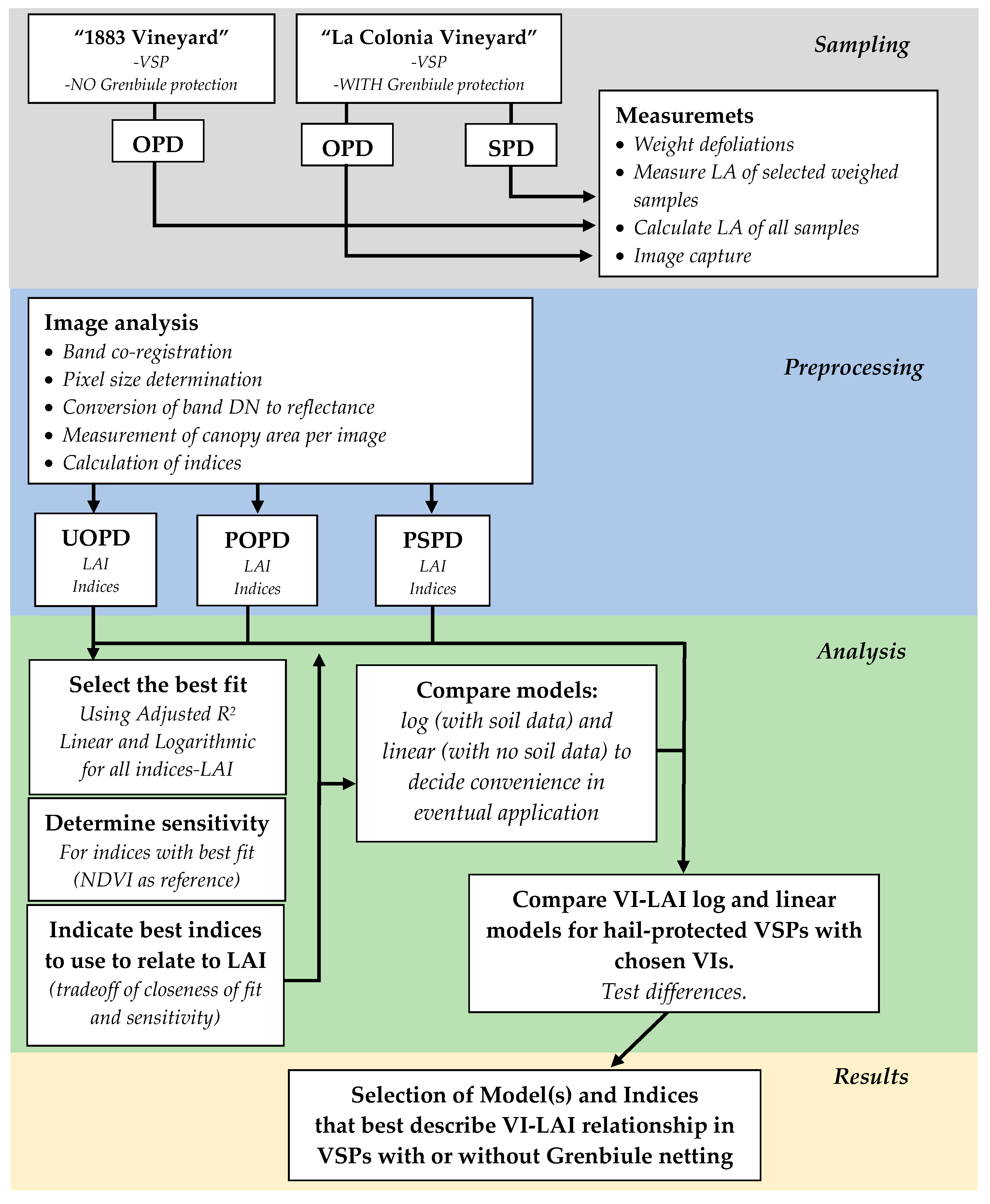
2. Materials and Methods

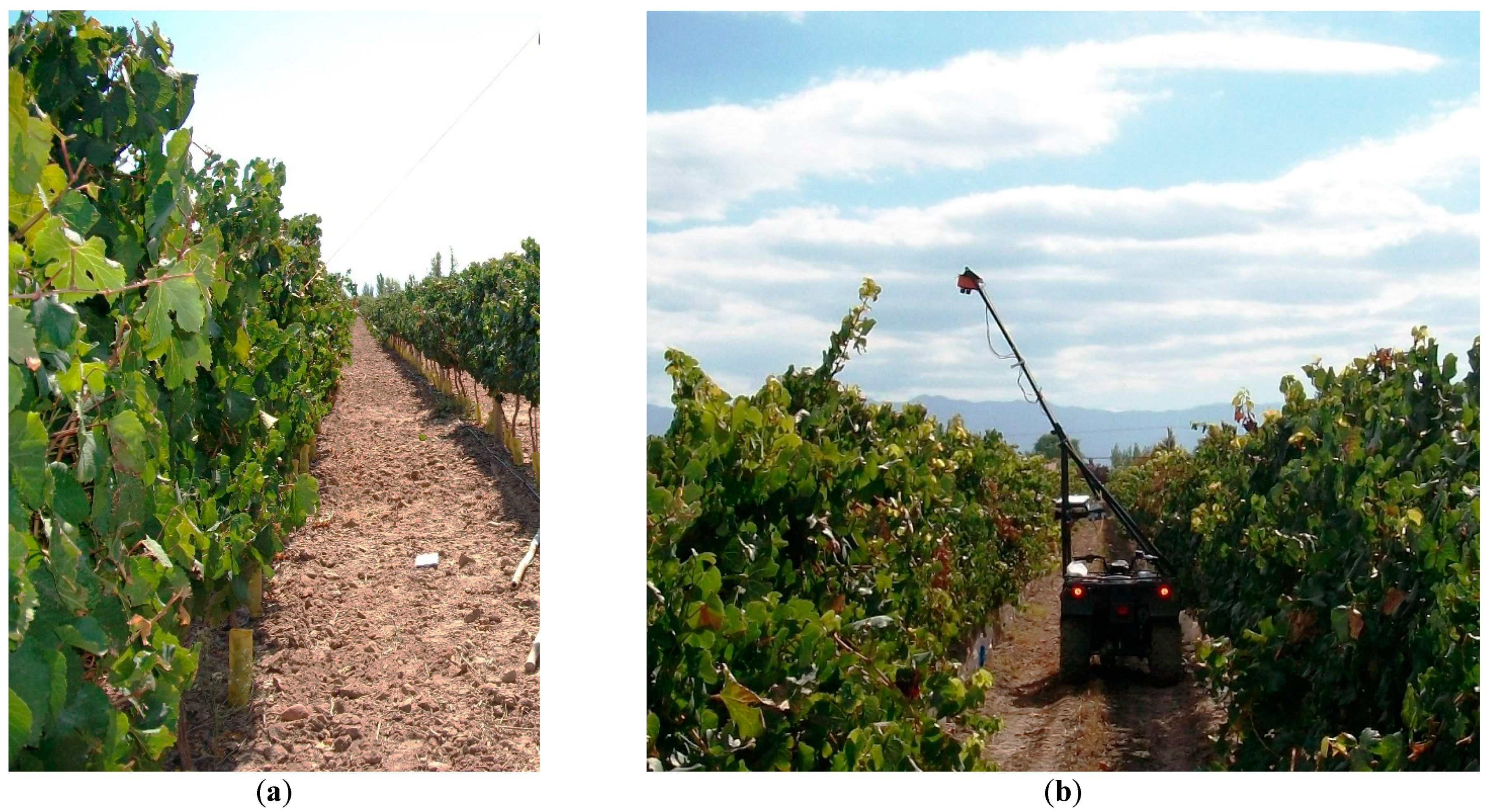
2.1. Description of the Study Sites

Field measurements were obtained shortly before the 2011 harvest from non-protected and protected Malbec VSPs at two sites. Site 1 was a non-protected Malbec located in the “1883” vineyard belonging to the Grupo Peñaflor in Coquimbito, Mendoza (lat.: 32°58′43″S, long.: 69°45′03″W, 770 m.a.s.l). Site 2 was a Grenbiule hail-netting protected Malbec located in the “La Colonia” vineyard belonging to Bodega Norton in Agrelo, Mendoza (lat.: 33°09′10″S, long.: 68°56′03″W, 970 m.a.s.l). Guided by the vineyard-managing viticulturists, four and five sampling sites with different vigour were chosen within Site 1 and 2, respectively. The sites are situated 27 km apart in an arid region subject to a monsoonal rain pattern with an average yearly rainfall of 265 mm, of which 150 mm falls between December and March. The maximum average temperature is 30 °C (December and January), with daily maxima often reaching over 40 °C. The coldest month (July) has a mean minimum temperature of 3 °C. Mean thermal amplitude in January averages 12 °C and 5.5 °C in July, while the yearly mean amplitude is 20.5 °C. Occasional early frost occurs in late April, and late frosts may occur until the end of October. From budburst to harvest, solar radiation adds to around 1.14 MW/m² and growing degree days (GDD) over a base temperature of 10 °C reaches 1600.

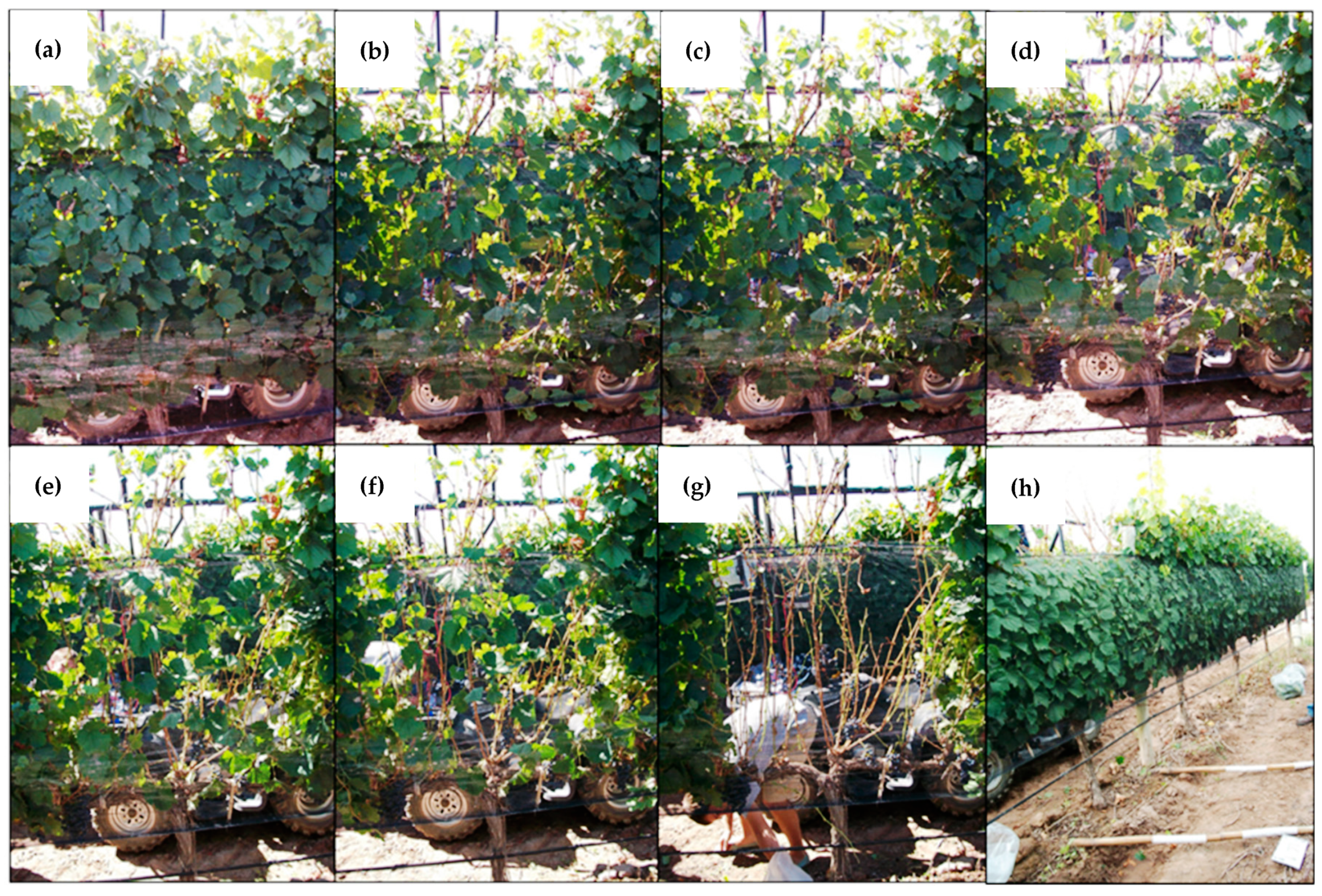
2.2. Canopy Leaf Distributions Generated with and without Hail Protection

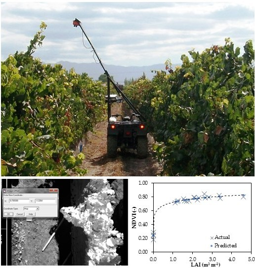
In the sectors with no hail-netting, successive images were taken, and between each acquisition the canopy was partially defoliated by hand, taking one of every four or five leaves along each shoot inside the camera IFOV, starting with the full canopy and ending with no leaves and an image of the underlying bare soil.

In the sectors with hail-netting, defoliation was carried out by two means:

(a) At two of the sampling areas, the procedure was identical to that with no netting: The vines were progressively defoliated, and the netting was replaced before each image capture (Figure 2a–g).

(b) At the other three sampling areas, progressive defoliation was performed on the shoot segments growing over the netting first and only then in the canopy inside the netting (Figure 2h).

The first method (overall progressive defoliation—OPD), simulates the canopy density in vines of different vigour as they reach maximum shoot elongation around Vèraison. The second (stepwise progressive defoliation—SPD) reproduces the effect of tipping after full canopy development, allowing evaluation of spectral response should the unconstrained shoots produce different reflectance values compared to the leaf area within the netting.

In summary, reflectance values were collected for three situations: (i) VSP with no hail protection and progressive, even defoliation (OPD); (ii) VSP with netting defoliated evenly as at the sites with no Grenbiule hail protection (OPD); and (iii) VSP with protection, and shoot tip (shoots growing over netting), progressively defoliated first, and the canopy inside the netting after (SPD). At each site, canes were placed along sun orientation and with markings to allow pixel size determination (Figure 2h).

2.3. LAI Estimation

The leaves collected at each defoliation at all sites were stored in individual black plastic bags and identified. They were kept in a refrigerated cooler and measurements were performed on them within two hours of field collection. All samples were weighed, and eight bags were randomly selected. From these bags, all leaves were distributed on the floor within an area of known size, photographed with a standard digital RGB camera, and the LA of each of the chosen samples was determined. LAI was then calculated dividing the accumulated LA of samples at each site by the canopy cover area measured by carefully delineating its extension on the corresponding NIR image using ERDAS Imagine (Hexagon Geospatial, Madison, AL, USA). A linear regression function of LA against weight (R² = 0.905) was calculated and used to determine the leaf area of all samples [34]. LAI was then calculated by dividing the LA of each sample by the canopy cover area measured by carefully delineating its surface on the NIR image in each case.

2.4. Spectral Data Acquisition

A Tetracam ADC (Tetracam Inc., Chatsworth, CA, USA) with four individual cameras fitted with spectral bandwidth filters in the green (G; 535–577 nm), red (R; 639–674nm), red edge (RE; 716–727 nm), and near-infrared (NIR; 755–900 nm) portions of the electromagnetic spectrum was used to capture nadir-view images over the canopy at each site, prior to each defoliation, over a single day at the beginning of March, approximately four weeks before harvest. In order to convert the digital number values of each band to reflectance, panels were made by painting chipboard tiles with different proportions of matt black and matt white paint, and then calculating their reflectance as a quotient of direct solar irradiance and nadir reflected light using a spectrometer (Ocean Optics, model SD2000 Ocean Optics, Largo, FL, USA). The multispectral camera was then set to the exposure time to be used in the field (one millisecond), and images were captured of each panel within two hours of midday. The digital numbers obtained for each panel were paired with the corresponding panel reflectance and OLS regression functions established with which to convert the image digital number values to reflectance. The camera was mounted on a boom designed to be fitted to a quadricycle (Figure 1b) and moved successively to each sampling site, where nadir-viewing images in all bands were captured with one-millisecond exposure time before each defoliation.

2.5. Multispectral Image Analysis

Band alignment with an affine pixel shift was performed on all individual band images at each site to force coincidence to a visible feature near the NIR scene centre to ensure that indices were calculated from values on matching points. Using ERDAS Imagine (Hexagon Geospatial, Madison, AL, USA), visible marks of known length on the marking canes in every image were used to determine pixel size, yielding average resolutions of 0.0022 m. A polygon delimiting a portion of the canopy, and another of the adjacent sunlit soil, were then carefully hand-drawn within each NIR image, and their area and brightness determined for all bands. LA per image averaged 1.92 m², so spectral calculations for VIs were performed with over 400,000 pixels per sample. As previously mentioned, the area was used to calculate LAI. Brightness values were converted to reflectance.

2.6. Vegetation Indices

Values obtained for canopy and soil at each site were used to compute the VIs. Typically, the VIs are calculated using commonly available R and NIR bands, with some exceptions, such as the chlorophyll index that requires red-edge (RE) in addition to NIR. NDVI is the most widely used index because of its robustness and insensitivity to atmospheric attenuation. However, it is susceptible to soil noise and insensitive to change at high values of biomass [18,29]. This aspect has promoted the development of several indices in an attempt to compensate for these shortcomings. The modified soil-adjusted vegetation indices (MSAVI and MSAVI₂) [24], soil-adjusted vegetation index 2 [35], and the perpendicular vegetation index (PVI) [36] are examples, but with the exception of MSAVI₂, they require knowledge of the gradient of the soil line [17], so all the data collected over sunlit soil at both vineyards were used in their determination (Figure 3). In the case of MSAVI, the determination of the L coefficient originally developed for SAVI (soil-adjusted vegetation index) is also required [24], but MSAVI₂ calculation avoids the need for a priori soil line determination. SAVI₂, MSAVI, and MSAVI₂ are examples of indices developed to minimise the effect of soil reflectance, as is PVI. The wide dynamic range vegetation index (WDRVI) [18] has been included due to its sensitivity to changes at high biomass and is calculated with two NIR weighting coefficients (α = 0.05 and α = 0.3). The inclusion of a chlorophyll index, CI_rededge, was considered because, aside from performing as a good LAI estimator in maize, it has been demonstrated to be a good estimator of gross primary production [25,37], and this would make it useful for VRB assessment, particularly since the recent availability of RE bands in several satellite-borne sensors. The VIs studied were selected among those that are widely used and that enhance sensitivity, reduce soil noise, employ either typical or unusual spectral bands, and are representative of different calculation procedures. The main characteristics of the VIs chosen for this study are listed in Table 1.

2.7. Data Analysis

Two models were selected to study each VI—LAI relationship: (i) A logarithmic model based on the light extinction functions common for vegetation as described by [3,38], and (ii) a linear model excluding bare soil values. The logarithmic model that considers light flux in the canopy may be represented by

$$\mathrm{Q}={\mathrm{Q}}_0{ \mathrm{e}}^{\left(-\mathrm{kL}\right)}$$

(1)

where Q is the radiation flux at any plane of the canopy, Q₀ is the incoming radiation at the top of the canopy, k is a parameter that combines the transmission coefficient for any given wavelength and a geometrical component accounting for leaf distribution and orientation, and L is the leaf area above the plane. The parameter k is often considered a constant for a given crop [38], as can the Q/Q₀ ratio at any given moment. As this ratio is associated to the fraction of photosynthetically active radiation that VIs are known to be closely associated with, considering this assumption and the exponential/logarithmic relationship between the dependent and independent variables, Equation (1) may be modified to

$$\mathrm{Vegetation} \mathrm{Index}={\mathrm{a}}_1\ln \left(\mathrm{LAI}\right)+{\mathrm{a}}_2$$

(2)

where, a₁, and a₂ are constants and ln(LAI) is the natural logarithm of the LAI.

Although the VI–LAI relationship over the full range from bare soil to maximum canopy density is inherently nonlinear, this generalisation does not hold for all VIs or the more commonly used ones above an LAI of 1 [25]. Above this value, the relationship is close to linear and may be expressed with a standard linear function such as

$$\mathrm{Vegetation} \mathrm{Index}={\mathrm{b}}_1\left(\mathrm{LAI}\right)+{\mathrm{b}}_2$$

(3)

where, b₁ and b₂ are constants.

Logarithmic and linear OLS regressions were performed using Infostat software (Infostat v.2016, Córdoba, Argentina). Data studied with the logarithmic model included the underlying soil data (i.e., no-leaf). LAI values below 1 correspond to a sparsely-leaved canopy, which is unlikely to be found in the field unless very soon after sprouting or severe canopy damage. Therefore, linear models were tested with no bare soil data.

All regression coefficients were studied for the unprotected canopy, and the VI exhibited the highest coefficient of determination with the logarithmic models employing all canopy and underlying soil data in unprotected VSPs, NDVI, was used as a benchmark reference for both the sensitivity study and the logarithmic analysis of hail-protected canopies. Following the approach described by Gitelson [8] for these comparisons, the first derivative of each logarithmic function with respect to ln(LAI), and the gradient b₁ of the linear functions obtained were used to compare each VI’s sensitivity, with NDVI as the reference, using the expression

$${\mathrm{S}}_{\mathrm{r}}=\left[\mathrm{d}\left(\mathrm{VI}\right)/\mathrm{d}\left(\mathrm{NDVI}\right)\right]{\left[\Delta \mathrm{VI}/\Delta \mathrm{NDVI}\right]}^{-1}$$

(4)

where Sr is the relative sensitivity, d(VI) and d(NDVI) are the first derivative of each VI and NDVI with respect to ln(LAI) (for the logarithmic functions) and the ratio of VI to NDVI gradients (for the linear functions), and Δ indicates each VI’s range of values.

With the aid of dummy variables, parameter significance for the LAI–VI regressions with both logarithmic and linear models, were tested for three canopy structures: (i) no protection, (ii) netting with shoots emerging over protection, and (iii) canopy entirely within the netting.

Finally, a schematic view of the whole procedure used in this study is illustrated in Figure 4.

3. Results

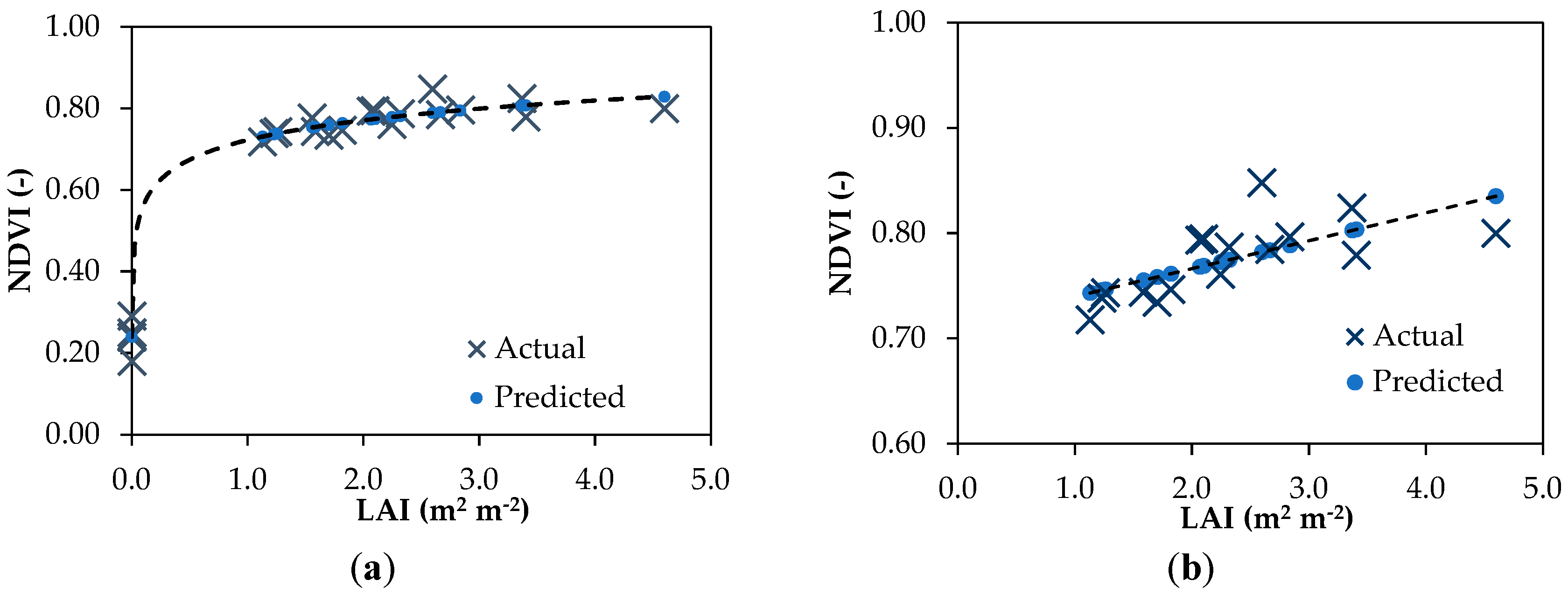
3.1. VI Accuracy Comparison

Table 2. Logarithmic and linear (with no-leaf values excluded) regression functions and their corresponding adjusted determination coefficient (R²) and root-mean-square error (RMSE) of leaf area index (LAI) prediction as a function of each vegetation index. Sampling areas with no hail netting.

Vegetation Index	Logarithmic Regression Model	Adjusted R2	RMSE	Linear Regression Model	Adjusted R2	RMSE
NDVI	0.069 ln(LAI) – 0.72	0.98	0.59	0.03 LAI + 0.71	0.48	0.61
WDRVI (1)	0.098 ln(LAI) + 0.33	0.97	0.87	0.06 LAI + 0.27	0.48	0.69
MSAVI2	0.064 ln(LAI) + 0.67	0.96	1.10	0.04 LAI + 0.63	0.36	0.71
WDRVI (2)	0.056 ln(LAI) – 0.47	0.91	2.71	0.05 LAI – 0.56	0.47	0.80
RVI	0.866 ln(LAI) + 7.48	0.83	5.63	1.02 LAI + 5.55	0.46	0.91
SAVI2	2.886 ln(LAI) + 21.10	0.73	10.04	4.93 LAI + 11.96	0.45	0.55
MSAVI	0.106 ln(LAI)+ 0.95	0.69	2.63	0.21 LAI + 0.58	0.33	0.80
PVI	0.027 ln(LAI) + 0.52	0.67	7.10	0.03 LAI + 0.46	0.15	0.89
CIrededge	0.056 ln(LAI) – 1.05	0.41	5.40	-	-	-

α is a coefficient applied to NIR values in the standard NDVI formula to reduce the ratio of NIR to R reflectance values, thus enhancing R absorption and sensitivity with high biomass or chlorophyll contents. (1) α = 0.3; (2) α = 0.05; RMSE, root-mean-square error; models with adjusted R² lower than 0.10 have been omitted.

shows the logarithmic, and linear regression functions with their adjusted R² for all the VIs tested as a function of LAI, at all sites with no hail protection. The root-mean-square error (RMSE) for LAI prediction from each VI is also shown.

Figure 5a,b show the logarithmic and linear LAI–VI regression plots that exhibit the highest adjusted R² values and correspond in both cases to NDVI.

3.2. VI Sensitivity to LAI Changes

Based on the convenience of using linear relationships within typical canopy LAI ranges, a comparison of the sensitivity of different indices to LAI was performed with the calculation of Sr, using NDVI as a reference. Only indices obtained from VI–LAI linear regressions where gradient parameter significance were used (p < 0.01). Results are detailed in

Table 3. Relative sensitivity (Sr) of indices with respect to LAI, with NDVI used as the reference.

Vegetation Index	Relative Sensitivity (Sr)
NDVI (Reference)	1.0
RVI	2.74
WDRVI (α = 0.05)	2.07
MSAVI2	1.45
WDRVI (α = 0.3)	1.42

.

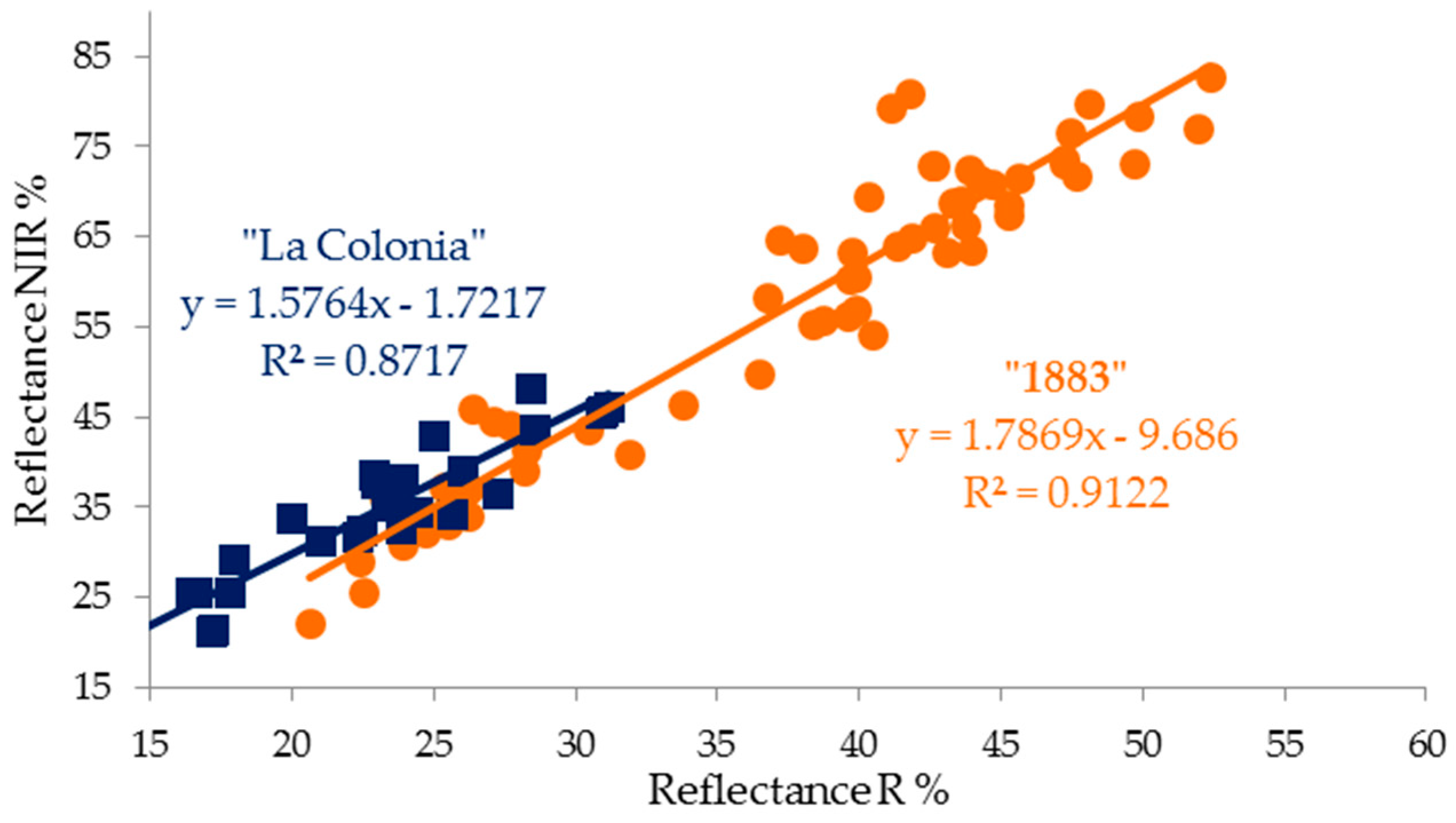
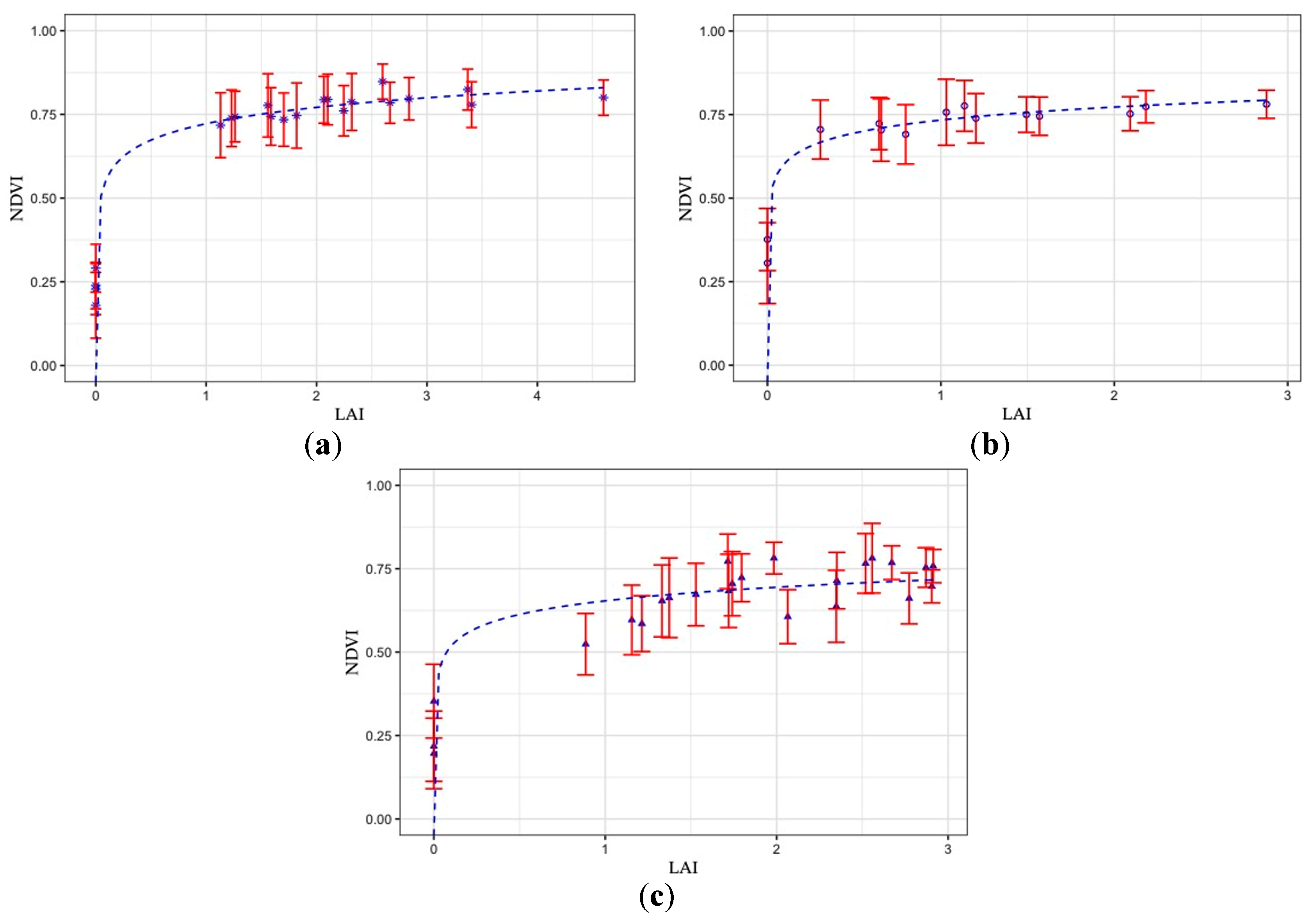
3.3. Effect of Grenbiule Hail-Protection Netting on the VI–LAI Relationship

For illustration purposes, comparison of the effects of the Grenbiule hail protection on the logarithmic LAI to NDVI relationship for “La Colonia” vineyard is shown in Figure 6, together with the sample canopy NDVI dispersion represented by one standard deviation. Results for three selected VIs (most accurate (NDVI), most sensitive (RVI), and best compromise (WDRVI)) with both linear and logarithmic models are detailed in

Table 4. Logarithmic regression parameter estimations and significance for all data, separated with auxiliary variables and unprotected canopy values as the reference.

	NDVI		WDRVI (α = 0.05)		RVI
Coefficient	Estimation	p-Value	Estimation	p-Value	Estimation	p-Value
Constant	0.72	<0.0001	−0.48	<0.0001	7.26	<0.0001
lnLAI	0.07	<0.001	0.05	<0.0001	0.83	<0.0001
POPD	0.01	0.3265	−0.02	0.3435	−0.5	0.1888
PSPD	−0.06	<0.0001	−0.01	<0.0001	−1.73	<0.0001
POPD_lnLAI	−0.01	0.0112	−0.01	0.2878	−0.13	0.3308
PSPD_lnLAI	0.0036	0.4518	−0.01	0.1026	−0.22	0.0874

POPD = protected, overall progressive defoliation; PSPD = protected, stepwise progressive defoliation.

and

Table 5. Linear regression parameter estimations and significance for all data, separated with auxiliary variables and unprotected canopy values as the reference.

	NDVI		WDRVI (α = 0.05)		RVI
Coefficient	Estimation	p-Value	Estimation	p-Value	Estimation	p-Value
Constant	0.72	<0.0001	−0.54	<0.0001	5.78	<0.0001
LAI	0.02	0.0212	0.05	0.0014	0.92	0.0004
POPD	−0.02	0.6117	−0.02	0.7242	−0.18	0.8194
PSPD	−0.19	<0.0001	−0.21	0.0001	−3.32	0.0005
POPD_LAI	0.01	0.6887	−0.0042	0.8640	0.0045	0.9916
PSPD_LAI	0.05	0.0021	−0.05	0.0443	0.61	0.1269

POPD = Protected, Overall Progressive Defoliation; PSPD = Protected, Stepwise Progressive Defoliation.

.

4. Discussion

4.1. VI Accuracy Comparison

Adjusted R² was used as a means to estimate the accuracy of the VIs. Results shown in Table 2 indicate that ratio indices are substantially more accurate than perpendicular or chlorophyll indices, some of which show very poor or no linear relationship whatsoever with LAI [3]. As the practical application of these relationships aims to estimate LAI as the dependent variable, the functions were inverted, and an RMSE for LAI was calculated, with similar results in order of accuracy (Table 2). Exclusion of bare soil values exposes the influence that the no-leaf data has in accuracy (R² = 0.48 for linear regression with no soil data vs. R² = 0.98 for the logarithmic function including soil values with NDVI). This effect is consistent with studies that have shown that at low vegetation cover values, soil backscattering can contribute to more signal than vegetation cover, particularly with some indices such as NDVI [24]. Moreover, inspection of the soil lines shown in Figure 3 illustrates that bare soil data can vary somewhat within the study region, which in turn would influence the y-intercept and regression functions obtained for otherwise identical canopies. From a practical standpoint, if RS data available have sufficient resolution to allow canopy values to be separated from soil values, the high LAI values typical of VSPs should occlude soil response and VIs adjusted for soil response would be expected to show little improvement in the accuracy of LAI estimation. In turn, this would preclude the need for soil line determination for the index calculation. However, SAVI₂ exhibits the lowest RMSE in LAI estimation with linear models that exclude bare soil values, a result that is difficult to interpret and needs to be addressed with further studies.

Logarithmic relationships are often accepted as a necessary consequence of extinction and other factors affecting light interception such as leaf orientation [3,38], and the results obtained here are strikingly similar to those obtained by Gitelson and others [15,25,39] in corn. However, the field measurements performed show that an LAI under 1.0 would imply extreme defoliation unlikely to be found in the field (Figure 5), or a canopy at a very early stage during the growing season [5]. In short, as soil reflectance will influence the y-asymptote and affect the regression function without providing added accuracy in standard canopies with LAI values above 1.0, the use of logarithmic regressions is impractical for viticulture use, and linear models are appropriate for this purpose [40].

4.2. VI Sensitivity to LAI Changes

The lack of sensitivity over an LAI of 2.0, commonly cited for NDVI and other indices [25], must be overcome for any useful application of VI–LAI regressions. Amongst those VIs tested, RVI exhibits the highest sensitivity to changes in LAI, lending support to the main reason for its widespread use in Australian viticulture. Differential harvesting and management applications using RVI block maps (often referred to as “Plant Cell Density”) have been shown to have a significant economic impact and to be significantly related to such crop characteristics as vine vigour, fruit sugar content, titratable acidity, and sensory quality assessment [22]. Both WDRVIs, explicitly developed to offset the lack of sensitivity NDVI exhibits at high LAI values, have significantly more Sr than NDVI but vary considerably depending on the NIR correction α coefficient applied. Even MSAVI₂ presents better Sr than NDVI, an unexpected finding considering its development was aimed specifically at correcting bias shown by NDVI with low vegetation cover. Its use has borne good results in orchard vegetation cover estimations [41] as well as in forest biomass estimations [42] and appears promising to estimate land cover in a sparsely vegetated area like shrubland. In summary, NDVI seems to be the least sensitive of the studied indices, even if the most accurate. These results suggest a WDRVI to be an adequate compromise between accuracy and sensitivity. This effect is in overall agreement with studies showing that in situations with dense green biomass (NDVI > 0.4), the sensitivity of the WDRVI may be 47% greater than that of the NDVI in several types of vegetation cover, including woodlands, sub-humid to humid grasslands, and croplands [29].

4.3. Effect of Grenbiule Hail-Protection Netting on the VI–LAI Relationship

As data were collected post-Vèraison, canopy size can be assumed to have reached full development [30]. OPD mimics LAI evolution and LA expansion throughout the season, even after shoots emerge over the netting, so it allows protected and unprotected canopies with similar leaf distribution to be compared. SPD imitates the structure of already fully developed canopies with different densities, including the leaves constrained within the netting and those that have grown over it. With this defoliation procedure, the shoots emerging outside the protection are progressively defoliated first, thus imitating tipping, a common management practice performed typically around Vèraison. Once all protruding shoot leaves are removed, it is also possible to compare the effect of the hail netting on the VIs of leaves entirely under protection and those completely exposed to sunlight.

As shown in Table 4 and Table 5, results obtained using dummy variables generated to test average VI values and the VI–LAI relationship under the three defoliation methods were similar: Average VI as a function of LAI did not differ significantly (p-value > 0.01) between protected and unprotected canopies with OPD. However, significant differences were found with protected canopy defoliated with SPD. As stated previously, OPD mimics canopy evolution, which includes early growth stages with low LAI values. Full canopy development within the hail netting may force leaf orientation, thus modifying the relationship after removal of the canopy that emerges over the netting and covers the protected leaves [38]. This effect may be enhanced for insensitive VIs, such as NDVI, at high canopy densities, as shown in Table 4.

Figure 6 reveals SPD differences to be greater at lower LAI values, that is, while most of the canopy is shaded by netting. This effect suggests that the canopy growing over the hail netting has a dominating effect on nadir-viewing VI canopy values. Furthermore, the differences between models may be more significant in the low LAI range, where linear regressions exhibit a poorer fit. For this reason, Table 4 and Table 5 include results for the three ratio vegetation indices of interest (NDVI (highest accuracy), RVI (highest sensitivity), and WDRVI (α = 0.05) (best compromise)) using both logarithmic and linear models, respectively. The VI–LAI slope, however, as shown by the test results on interactions, shows no significant differences between models except NDVI in the logarithmic model, plausibly for the reasons postulated above. Despite similar slopes, values under netting exhibit a considerable offset, so use of different linear relationships may be warranted. The offset over an LAI of 1.0 evidenced in Figure 6 suggests that hail protection netting indeed reduces VI values obtained for a given LAI, particularly during initial growth stages. However, any difference would gain importance as the canopy approaches its final size. Despite the existing difference, it is yet unclear whether the netting material differentially affects light quality in the wavelengths required for index extraction, as the results would imply, or if canopy confinement and shading affect its density, condition or leaf orientation, and therefore its spectral response. Nevertheless, OPDs with and without protection yield nearly identical regression functions, so the choice of the relationship to use would depend either on overall canopy density or addressed as a situation exhibiting some form of hysteresis, depending on whether the canopy is actively growing or has reached the final size after Vèraison.

5. Conclusions

Ratio vegetation indices such as NDVI, RVI, and the WDRVIs exhibited a closer relationship with pure canopy LAI than the perpendicular (PVI), mixed (SAVI₂ and MSAVIs) and the chlorophyll index (CI_rededge). NDVI exhibited the highest accuracy. Logarithmic models, including the no-leaf values at each site, presented very high adjusted R² values (over 0.80), but values above an LAI of one followed a linear distribution. Considering that LAI values above 1 occlude direct soil reflectance and that pure canopy field values are commonly well above this value, a linear model for the VI–LAI relationship is acceptable above this value and avoids possible soil contribution to canopy values. This effect is desirable because soil lines in the same area may vary.

The sensitivity of NDVI was considerably lower than those of other ratio indices, while RVI shows the highest sensitivity. Because RVI has indicated a low accuracy, a good alternative would be to adopt WDRVI. This index indicates a superior sensitivity with a stronger weighting of the NIR values (i.e., α = 0.05 is better that α = 0.3), but the optimum weighting coefficient has not been determined.

Hail-protection Grenbiule netting reduces VI values for a given LAI. Tipping practices enhance this effect in fully developed canopies. Results suggest the same VI–LAI relationship holds for protected and unprotected canopies in the initial vegetation stages, but different functions are preferable once the canopy is fully developed, in particular, if tipping is executed.

References

1. Ravaz, M.L. L’effeuillage de la vigne. Annales de L’Ecole Nationale d’agriculture de Montpellier 1911, 11, 216–244. [Google Scholar]
2. Watson, D.J. Comparative Physiological Studies on the Growth of Field Crops: I. Variation in Net Assimilation Rate and Leaf Area between Species and Varieties, and within and between Years. Ann. Bot. 1947, 11, 41–76. [Google Scholar] [CrossRef]
3. Milthorpe, F.L.; Moorby, J. An Introduction to Crop Physiology; Cambridge University Press: Cambridge, UK, 1974. [Google Scholar]
4. Hall, A.; Lamb, D.W.; Holzapfel, B.; Louis, J. Optical remote sensing applications in viticulture—A Review. Aust. J. Grape Wine Res. 2002, 8, 36–47. [Google Scholar] [CrossRef]
5. Johnson, L.F. Temporal stability of an NDVI-LAI relationship in a Napa Valley vineyard. Aust. J. Grape Wine Res. 2003, 9, 96–101. [Google Scholar] [CrossRef] [Green Version]
6. Hall, A.; Lamb, D.; Holzapfel, B.P.; Louis, J.P. Within-season temporal variation in correlations between vineyard canopy and winegrape composition and yield. Precis. Agric. 2011, 12, 103–117. [Google Scholar] [CrossRef]
7. Towers, P.C.; Strever, A.; Poblete-Echeverría, C. Estimation of Vine Pruning Weight using Remote Sensing Data: Relative Contribution of Variables. In Proceedings of the 20th GiESCO International Meeting, Mendoza, Argentina, 5–10 November 2017. [Google Scholar]
8. Howell, G.S. Sustainable Grape Productivity and Growth-Yield Relationship: A Review. Am. J. Enol. Vitic. 2001, 52, 165–174. [Google Scholar]
9. Kliewer, W.M.; Dokoozlian, N.K. Leaf area/crop Weight ratios of grapevines: Influence on fruit composition and wine quality. Am. J. Enol. Vitic. 2005, 56, 170–181. [Google Scholar]
10. Bramley, R.G.V. Understanding variability in winegrape production systems-2. Within vineyard variation in quality over several vintages. Aust. J. Grape Wine Res. 2005, 11, 33–42. [Google Scholar] [CrossRef]
11. Rydberg, A.M. Potential Crop Growth Assessment from Remotely Sensed Images Compared to Ordinary Yield Maps. In Proceedings of the Fifth International Conference on Precision Agriculture, Bloomington, MN, USA, 16–19 July 2000. [Google Scholar]
12. Machado, S.; Bynum, E.D., Jr.; Archer, T.L.; Lascano, R.J.; Bordovsky, J.; Bronson, K.; Nesmith, D.M.; Segarra, E.; Rosenow, D.T.; Peterson, G.C.; et al. Spatial and temporal variability of sorghum and corn yield: Interactions of biotic and abiotic factors. In Proceedings of the Fifth International Conference on Precision Agriculture, American Society of Agronomy, Bloomington, MN, USA, 16–19 July 2000. [Google Scholar]
13. Kravchenko, A.N.; Robertson, G.P.; Thelen, K.D.; Harwood, R.R. Management, Topographical, and Weather Effects on Spatial Variability of Crop Grain Yields. Agron. J. 2005, 97, 515–523. [Google Scholar] [CrossRef]
14. Hall, A.; Louis, J.P.; Lamb, D.W. Low-resolution remotely sensed images of winegrape vineyards map spatial variability in planimetric canopy area instead of leaf area index. Aust. J. Grape Wine Res. 2008, 14, 9–17. [Google Scholar] [CrossRef]
15. Walthall, C.L.; Pachepsky, Y.; Dulaney, W.P.; Timlin, D.J.; Daughtry, C.S.T. Exploitation of spatial information in high resolution digital imagery to map leaf area index. Precis. Agric. 2007, 8, 311–321. [Google Scholar] [CrossRef] [Green Version]
16. Poblete-Echeverría, C.; Olmedo, G.F.; Ingram, B.; Bardeen, M. Detection and Segmentation of Vine Canopy in Ultra-High Spatial Resolution RGB Imagery Obtained from Unmanned Aerial Vehicle (UAV): A Case Study in a Commercial Vineyard. Remote Sens. 2017, 9, 268. [Google Scholar] [CrossRef]
17. Jackson, R.D.; Huete, A.R. Interpreting Vegetation Indices. Prev. Vet. Med. 1991, 11, 185–200. [Google Scholar] [CrossRef]
18. Gitelson, A.A. Wide Dynamic Range Vegetation Index for Remote Quantification of Biophysical Characteristics of Vegetation. J. Plant Physiol. 2004, 161, 165–173. [Google Scholar] [CrossRef] [PubMed]
19. Huete, A.R. A Soil-Adjusted Vegetation Index (SAVI). Remote Sens. Environ. 1988, 25, 295–309. [Google Scholar] [CrossRef]
20. Qi, J.; Kerr, Y.; Chehbouni, A. External factor consideration in vegetation index development. In Proceedings of the 6th International Symposium on Physical Measurements and Signatures in Remote Sensing, Val D’Isere, France, 17–22 January 1994; pp. 723–730. [Google Scholar]
21. Ray, T.W. A FAQ on Vegetation in Remote Sensing. Division of Geological and Planetary Sciences, California Institute of Technology. 1994. Available online: http://www.yale.edu/ceo/Documentation/rsvegfaq.html (accessed on 15 August 2018).
22. Proffitt, T.; Pearse, B. Adding value to the wine business precisely: Using precision viticulture technology in Margaret River. Managing vineyard variation—Precision viticulture workshop. In Proceedings of the 12th Australian Wine Industry Technical Conference; The Australian and New Zealand Grapegrower and Winemaker: Broadview, Australia, 2004; pp. 40–44. [Google Scholar]
23. Richardson, A.J.; Wiegand, C.L. Distinguishing vegetation from soil background information. Photogramm. Eng. Remote Sens. 1977, 43, 1541–1552. [Google Scholar]
24. Qi, J.; Chehbouni, A.; Huete, A.R.; Kerr, Y.H.; Sorooshian, S. A Modified Soil Adjusted Vegetation Index. Remote Sens. Environ. 1994, 48, 119–126. [Google Scholar] [CrossRef]
25. Gitelson, A.A.; Viña, A.; Arkebauer, T.J.; Rundquist, D.C.; Keydan, G.P.; Leavitt, B. Remote estimation of leaf area index and green leaf biomass in maize canopies. Geophys. Res. Lett. 2003, 30. [Google Scholar] [CrossRef] [Green Version]
26. Steele, M.R.; Gitelson, A.A.; Rundquist, D. Nondestructive Estimation of Leaf Chlorophyll Content in Grapes. Am. J. Enol. Vitic. 2008, 59, 299–305. [Google Scholar]
27. Gitelson, A.A.; Kaufman, Y.J.; Stark, R.; Rundquist, D. Novel algorithms for remote estimation of vegetation fraction. Remote Sens. Environ. 2002, 80, 76–87. [Google Scholar] [CrossRef] [Green Version]
28. Viña, A.; Henebry, G.M.; Gitelson, A.A. Satellite monitoring of vegetation dynamics: Sensitivity enhancement by the wide dynamic range vegetation index. Geophys. Res. Lett. 2004, 31. [Google Scholar] [CrossRef] [Green Version]
29. Keller, M. The Science of Grapevines. Anatomy and Physiology; Academic Press: London, UK, 2010; pp. 125–158. [Google Scholar]
30. Hatfield, J.L.; Gitelson, A.A.; Schepers, J.S.; Walthall, C.L. Application of Spectral Remote Sensing for Agronomic Decisions. Agron. J. 2008, 100, S-117–S-131. [Google Scholar] [CrossRef]
31. Bannari, A.; Morin, D.; Bonn, F.; Huete, A.R. A review of vegetation indices. Remote Sens. Rev. 1995, 13, 95–120. [Google Scholar] [CrossRef]
32. Lobos, G.A.; Poblete Echeverría, C. Spectral Knowledge (SK-UTALCA): Software for Exploratory Analysis of High-Resolution Spectral Reflectance Data on Plant Breeding. Front. Plant Sci. 2017, 7, 1996. [Google Scholar] [CrossRef] [PubMed]
33. Chanda, S.V.; Singh, Y.D. Estimation of Leaf Area in Wheat Using Linear Measurements. Plant Breed. Seed Sci. 2002, 46, 75–79. [Google Scholar]
34. Broge, N.H.; Leblanc, E. Comparing prediction power and stability of broadband and hyperspectral vegetation indices for estimation of green leaf area index and canopy chlorophyll density. Remote Sens. Environ. 2000, 76, 156–172. [Google Scholar] [CrossRef]
35. Wiegand, C.L.; Richardson, A.J.; Escobar, D.E.; Gerbermann, A.H. Vegetation Indices in Crop Assessments. Remote Sens. Environ. 1991, 35, 105–119. [Google Scholar] [CrossRef]
36. Peng, Y.; Gitelson, A.A.; Keydan, G.; Rundquist, D.C.; Moses, W. Remote estimation of gross primary production in maize and support for a new paradigm based on total crop chlorophyll content. Remote Sens. Environ. 2011, 115, 978–989. [Google Scholar] [CrossRef]
37. Glenn, E.P.; Huete, A.R.; Nagler, P.L.; Nelson, S.G. Relationship Between Remotely-sensed Vegetation Indices, Canopy Attributes and Plant Physiological Processes: What Vegetation Indices Can and Cannot Tell Us About the Landscape. Sensors 2008, 8, 2136. [Google Scholar] [CrossRef]
38. Carlson, T.N.; Ripley, D.A. On the relation between NDVI, fractional vegetation cover, and leaf area index. Remote Sens. Environ. 1997, 62, 241–252. [Google Scholar] [CrossRef]
39. Johnson, L.F.; Roczen, D.; Youkhana, S. Vineyard Canopy Density Mapping with IKONOS Satellite Imagery. In Proceedings of the Third International Conference on Geospatial Information in Agriculture and Forestry, Denver, CO, USA, 5–7 November 2001. [Google Scholar]
40. Perry, A.; Weber, K. Land Cover Change Analysis Using MSAVI2 for Orchard Project; Orchard LCC Project 2015; Idaho State University: Pocatello, ID, USA, 2015. [Google Scholar]
41. Laosuwan, T.; Uttaruk, Y. Estimating Tree Biomass via Remote Sensing, MSAVI 2, and Fractional Cover Model. IETE Tech. Rev. 2014, 31, 362–368. [Google Scholar] [CrossRef]
42. Ahmad, F. Spectral vegetation indices performance evaluated for Cholistan Desert. J. Geogr. Reg. Plan. 2012, 5, 165–172. [Google Scholar]
Figure 1. (a) Example of a vertically shoot positioned (VSP) vineyard (cv. Malbec); (b) Tetracam ADC multispectral camera mounted on a boom on a quadricycle in preparation for a nadir-viewing capture on the canopy in a VSP vineyard.
Remotesensing 11 01073 g001
Figure 2. Defoliation procedure: (ag) Progressive uniform defoliation of a hail-protected VSP, removing the netting to implement the defoliation (netting was reinstalled before each image capture); and (h) Stepwise progressive defoliation of a hail-protected VSP; in this case, the netting remained installed and shoot tips extending over the net were defoliated first to simulate tipping, and canopy under the netting was defoliated later.
Remotesensing 11 01073 g002
Figure 3. Soil lines for the two sites used in this study: (orange) soil line for Site 1 and (blue) soil line for Site 2. The linear regression function gradient obtained from plotting R against NIR reflectance of sunlit soil is used to calculate the perpendicular vegetation index (PVI), the Modified soil-adjusted vegetation index (MSAVI), and the Soil-adjusted vegetation index 2 (SAVI2).
Remotesensing 11 01073 g003
Figure 4. Schematic view of the full procedure used in this study.
Remotesensing 11 01073 g004
Figure 5. Regression of NDVI as a function of LAI: (a) Logarithmic; and, (b) linear.
Remotesensing 11 01073 g005
Figure 6. Logarithmic regressions of NDVI as a function of LAI including bare soil values, for VSPs with and without hail protection and different defoliation strategies: (a) UOPD—unprotected overall progressive defoliation (same curve presented in Figure 5a, this figure was included to aid with the comparisons), (b) POPD—protected overall progressive defoliation, and (c) PSPD—protected stepwise progressive defoliation. Bars indicate one standard deviation of the canopy NDVI values of each sample.
Remotesensing 11 01073 g006