Potential of Sentinel-1 C-Band Time Series to Derive Structural Parameters of Temperate Deciduous Forests

Abstract

With the increasing occurrence of forest fires in the mid-latitudes and the alpine region, fire risk assessments become important in these regions. Fuel assessments involve the collection of information on forest structure as, e.g., the stand height or the stand density. The potential of airborne laser scanning (ALS) to provide accurate forest structure information has been demonstrated in several studies. Yet, flight acquisitions at the state level are carried out in intervals of typically five to ten years in Central Europe, which often makes the information outdated. The Sentinel-1 (S-1) synthetic aperture radar mission provides freely accessible earth observation (EO) data with short revisit times of 6 days. Forest structure information derived from this data source could, therefore, be used to update the respective ALS descriptors. In our study, we investigated the potential of S-1 time series to derive stand height and fractional cover, which is a measure of the stand density, over a temperate deciduous forest in Austria. A random forest (RF) model was used for this task, which was trained using ALS-derived forest structure parameters from 2018. The comparison of the estimated mean stand height from S-1 time series with the ALS derived stand height shows a root mean square error (RMSE) of 4.76 m and a bias of 0.09 m on a 100 m cell size, while fractional cover can be retrieved with an RMSE of 0.08 and a bias of 0.0. However, the predictions reveal a tendency to underestimate stand height and fractional cover for high-growing stands and dense areas, respectively. The stratified selection of the training set, which we investigated in order to achieve a more homogeneous distribution of the metrics for training, mitigates the underestimation tendency to some degree, yet, cannot fully eliminate it. We subsequently applied the trained model to S-1 time series of 2017 and 2019, respectively. The computed difference between the predictions suggests that large decreases in the forest height structure in this two-year interval become apparent from our RF-model, while inter-annual forest growth cannot be measured. The spatial patterns of the predicted forest height, however, are similar for both years (Pearson’s R = 0.89). Therefore, we consider that S-1 time series in combination with machine learning techniques can be applied for the derivation of forest structure information in an operational way.

1. Introduction

The area of globally burnt forests, grasslands, and croplands caused by wildfires amounts to 3.3 to 3.8 million km${}^2$ per year [1,2]. Large amounts of greenhouse gases are emitted by fires [3,4,5] thereby altering atmospheric composition [6,7]. In the past, major wildfires predominantly occurred on the African continent, Australia and Brazil [1], but showed an increasing trend in occurrence and severity also in California and Siberia [8,9] and increasingly affect forest ecosystems in Central Europe due to climate change [9,10,11].

Occurrences of forest fires are a complex phenomenon. Physical and environmental conditions such as weather conditions [12,13], topography and fuel [14] were found to control the fire risk. Fire ignition events, on the other hand, can have natural causes like lightning, but human impacts are the major factor in Central Europe [15,16].

Fire risk assessments encompass two elements, namely the risk of fire ignition and fire propagation [17]. Knowledge of the horizontal and vertical vegetation structure is vital for such assessments as the fuel structure defines the preconditions for both of these components [18,19,20]. Structure information of fire-relevant forest properties has been derived from airborne laser scanning (ALS) data in the past, since ALS captures the forest structure at a high level of detail and provides a three-dimensional representation of the land surface. ALS allows the derivation of tree species (e.g., [21,22,23]), information on the forest layering including the characteristics of the understory (e.g., [24,25,26,27]), crown base height and crown length (e.g., [28,29,30]), canopy density related metrics such as crown coverage, and distribution and size of forest gaps [31,32,33].

A disadvantage of ALS, however, is its limited temporal resolution due to the high organizational and financial resources required. Therefore, county wide ALS acquisition missions are carried out in time intervals of 5 to 10 years, typically, which implies that the derived forest structure does not necessarily correspond to the situation today. Fire risk assessments, thus, would benefit if the forest structure was derived from more recent data.

Spaceborne synthetic aperture radar (SAR) missions have the potential to overcome the disadvantage of the low temporal resolution inherent to ALS data. SAR is an active microwave remote sensing technique which allows for the acquisition of vegetation structure information independently of daylight and weather conditions [34,35,36].

SAR data have been widely used in the past for the estimation of forest stand related parameters. A comprehensive overview on methods to derive the respective measures is given by Kaasalainen [37]. Two conceptually different methods can be distinguished, namely the inversion of SAR scattering models, and machine learning techniques. In the former concept, a scattering model is established, which relates the measured SAR interferometric coherence to structure properties [38,39,40]. Based on such models, stand height, for instance, could be retrieved from L-band (e.g., [39,40,41]), X-band (e.g., [42,43,44]), or C-band interferometric data [38]. SAR scattering models can also be applied for the derivation of forest cover related information from L-band and P-band [45] as well as from X-band interferometric data [43].

Independent of the quality of those methods, some of these studies deployed experimental systems, what hampers the operational application for forest surveys and monitoring. With the increasing availability of open EO data, machine learning approaches are coming into focus, which relate field-observed forest structure metrics and data-derived metrics. As demonstrated by Morin [46] or Li [47], for instance, machine learning frameworks allow for the combination of multiple sensor systems and offer the possibility to use a wide range of predictor metrics computed from the respective data sets, which have a known sensitivity to the forest structure. In particular, these two studies investigated the derivation of, inter alia, the stand height from P-band and C-band backscatter information. Urbazaev [48], finally, used multi-temporal and polarimetric information from L-band to predict woody cover using machine learning techniques.

Potential predictors also encompass time series metrics, which were demonstrated to be valuable for the derivation of structure-related forest parameters, such as forest type [35,36,49] and woody cover [50].

In our study, we follow up on these studies and gauge the potential of Sentinel-1 (S-1) C-band time series information for the derivation of forest structure metrics. S-1 carries a C-band SAR sensor, operating at a frequency of 5.4 GHz [51]. The disadvantage of such short wavelengths is their reduced ability to penetrate into the canopy [52,53]. As the system, therefore, is more sensitive to upper canopy layers, not all of the structure elements relevant for fire risk assessments are retrievable from S-1 data. It can only be expected to derive structure metrics related to the upper height layers. In our study, we, thus, focus on the derivation of the stand height and the fractional cover, which is a measure of the stand density.

Stand height is related to the canopy fuel, and its derivation from ALS data in the context of fire risk assessments has been addressed in the past (e.g., [54,55]). Canopy density controls the light regime with less dense canopies having a higher light transmission [56,57]. Increased solar irradiance on the forest floor, again, reduces the fuel moisture, thereby increasing the fire ignition risk [58]. Since the introduction of the fractional cover metrics computation from ALS data [59,60,61], its applicability for the characterization of the canopy density has been widely investigated and its consistency in particular with the canopy coverage has been proven (e.g., [33,57,62]). We therefore considered the fractional cover to be another key parameter in fire risk assessments and defined it as target metric which we want to derive from S-1.

SAR constellations like TanDEM-X, where two SAR scenes of the same spot are acquired simultaneously from two platforms flying in a close formation, allow for acrosstrack interferometry. Such a technique can be used to derive accurate estimates of forest height [63,64,65,66]. In contrast, the S-1 constellation allows for along-track interferometry [51]. However, the time interval between two acquisitions causes temporal decorrelation of the phase information, which impedes the formation of interferograms over vegetated areas. This temporal decorrelation is, among others, a function of vegetation cover and is expressed in the form of the interferometric coherence (e.g., [53,67]). Different approaches are therefore required for forest structure estimation. In our study, we test the feasibility of retrieving forest parameters from S-1 data deploying machine learning techniques, as such methods are straightforward to apply and would make open access earth observation (EO) data available to a wider circle of users. We follow up on the work by Morin [46] and Li [47]. However, in contrast to these studies, we use data from S-1 alone, which further simplifies the approach. We analyze to which degree the estimates of the forest structure parameters based on S-1 data solely match those from ALS data. For the estimation of structure metrics from S-1 time series, a random forest (RF) regression model is trained. Based on this model we test the potential of S-1 time series for the derivation of the desired structure metrics and investigate potential improvements in the training phase of the model. A further difference to the aforementioned studies is that we also use interferometric coherence as a predictor. Finally, the robustness of our model is tested by applying it to different years. Forest structure metrics computed from the ALS data set served as reference data in our study.

2. Material and Methods

2.1. Study Area

The study was carried out over the Wienerwald, located south-west of Vienna, Austria. The area is dominated by hills with heights between 200 m and 700 m above sea level. Forest is the main land cover type, with beech (Fagus sylvatica), oak (Quercus spp.) and hornbeam (Carpinus betulus) being the dominating species [68]. For our study, we selected a 16 × 6 km${}^2$ subset of the area, which is mainly covered by deciduous forest (Figure 1). Forest stand heights within the study area range up to 45 m, with a mean height of 17.8 m.

Our experiments were restricted to forest areas in order to avoid biases through settlement areas. The official forest mask from the Austrian Research Centre for Forests (BFW) for the federal state of Niederösterreich was used for the selection of forest areas, which was available in a 10 m raster grid. We considered a respective cell on the level of the target resolutions (i.e., 20 m, 40 m, 100 m) as forested, if at least 30% of the 10 m cells lying within a respective cell of the target resolution were classified as forest. With this aggregation approach of the forest mask, we fulfil the official forest definition of Austria [69].

2.2. ALS Data

ALS data were acquired on 20 September 2018 using a Riegl VQ-1560i sensor (RIEGL Laser Measurement Systems, Horn, Austria). The sensor operates with two independent laser channels, which results in scan lines tilted by ±14${}^{\circ }$ from the flight direction’s perpendicular axis [70]. Both lasers operated at a wavelength of 1064 nm. During the flight mission, an area of 53 × 8 km${}^2$ was captured by 18 strips with a side overlap > 50%, covering the city of Vienna and Wienerwald forest. The average flight altitude was 750 m above ground at a flight speed of 60 m/s. The pulse repetition rate was set to 1.33 MHz.

The point cloud was clipped to the study area (Section 2.1; Figure 1). The point records of both channels were used, which resulted in average point densities above forested areas of 82–108 points/m${}^2$.

2.3. ALS Data Processing

An overview of the ALS data processing is given in Figure 2. The ALS point cloud was normalized and reprojected from UTM 33 into the Equi7 Grid (cf., [71]) previous to the derivation of the structure metrics in order to match the S-1 products. The transformation of the ALS structure grids subsequent to their computation in UTM 33 would have involved an interpolation, what would have modified the structure information. Therefore, the initial transformation of the point cloud into the target reference system is more appropriate.

The entire point cloud processing was performed in the OPALS software package [72].

2.3.1. Stand Height

A normalized digital surface model (nDSM) at a spatial resolution of 1 m formed the basis for the derivation of the stand height. A DSM was computed from the point cloud through the approach described in Hollaus (2010) [73], which afterwards was normalized using a digital terrain model. The stand height, finally, was calculated by aggregating the nDSM values to the target resolution, for which we applied cell sizes of 20, 40 and 100 m, respectively, in our experiments. We tested four different calculation modes for the aggregation of the nDSM and summarized the stand height of a respective cell on the target resolution as the mean, the 50%-, 75%- and 95%-height quantile of the nDSM values falling within the cell area.

2.3.2. Fractional Cover

Fractional cover measures the fraction of ground which is covered by the forest canopy within a certain area and was computed following Morsdorf (2006) [60] as:

$$fractionalcover=\frac{N_{canopy}}{N_{total}}$$

(1)

where $N_{canopy}$ corresponds to the number of canopy points and $N_{total}$ to the total number of points within each cell. A height of 3 m above terrain was used as lower canopy threshold to distinguish canopy and ground points. Again, cell sizes of 20, 40, and 100 were selected for the computation.

2.4. Sentinel-1 Data

The second major input data set was C-band data from S-1 at 10 m pixel spacing. For this study, we used Level 1b high-resolution ground range detected (GRDH) and Level 1a single look complex (SLC) scenes, which were acquired in the Interferometric Wide (IW) swath mode. A total of 36 variables (

Table 1. Overview of the S-1 time series products used as predictor variables in our models. Slope and correlation refer to the backscatter-incidence angle relationship (Section 2.4.5). FM, JJA, ON refer to the time span over which the respective products where temporally aggregated and correspond to the months February–March, June–July–August, and October–November, respectively (Section 2.4.4).

Product Name	Temporal Aggregation	Separate for Each Orbit	Number of Products
VV backscatter	FM, JJA, ON, year	yes	8
VH backscatter	FM, JJA, ON, year	yes	8
Cross ratio VH/VV	FM, JJA, ON, year	yes	8
Coherence	FM, JJA, ON, year	yes	8
Slope VV	year	no	1
Slope VH	year	no	1
Correlation VV	year	no	1
Correlation VH	year	no	1
Total number of products			36

) were derived from S-1 using relative orbits 22 (descending) and 146 (ascending) to supply the structure prediction model (cf. Section 2.5) with input features being sensitive to the forest canopy structure at a fine scale. This includes parameters, which have already proven successful for vegetation or crop monitoring, e.g., radiometric terrain flattened Gamma Nought (${\gamma }_{rtf}$), cross ratio (CR) (e.g., [74,75,76]), coherence $\gamma$ (e.g., [77,78,79]), and the backscatter-incidence angle slope and correlation (e.g., [35,80]). Their meaning, characteristics, and processing procedure are described in more detail in the subsequent sections. An overview of the main processing steps for the retrieval of the backscatter products is given in Figure 3.

2.4.1. Radiometric Terrain Flattened Gamma Nought (Backscatter)

Radiometric terrain flattened Gamma Nought (herein denoted as ${\gamma }_{rtf}$) has become an indispensable backscatter variable for a vast amount of applications over complex terrain [36,81,82]. It stems from the novel radiometric terrain flattening algorithm presented in Small (2011) [83], where terrain effects are compensated by integrating the local illuminated area, projecting it into the radar geometry, and applying it as a reference area during radiometric normalization. The value of geo-referenced backscatter, i.e., Sigma Nought or Gamma Nought (herein denoted as ${\sigma }^0$ and ${\gamma }^0$, respectively), for forest area or type estimation has already been proven in the past [35,84]. However, obtaining reliable results in steep topography remained challenging, due to SAR effects like foreshortening, layover and shadowing, and those areas have therefore been masked. In comparison to such non radiometric terrain flattened backscatter variables, Rüetschi [36] could clearly show the benefit of using ${\gamma }_{rtf}$ over ${\gamma }^0$ for forest applications in complex terrain. Building upon these findings, we decided to select a high-resolution ${\gamma }_{rtf}$ data set covering our region of interest. Such a data set was available within the frame of the Austrian Data Cube (ACube [85]) project, which aims for establishing a service for the Austrian earth observation user community. The ingestion into the data cube was conducted using the SAR Geophysical Retrieval Toolbox (SGRT v2.4, cf. Naeimi [86]). During pre-processing, it invokes several modules from the Sentinel Application Platform (SNAP [87]) to apply (1) precise orbit data (2) border-noise removal (3) radiometric terrain flattening and (4) Range-Doppler terrain correction on Sentinel-1 IW GRDH scenes. A high-resolution terrain model [88] at 10 m pixel spacing was utilised during step (3) and (4) allowing to diminish terrain effects in ${\gamma }_{rtf}$ as best as possible.

2.4.2. Cross Ratio

The cross ratio (CR) corresponds to the ratio between ${\gamma }_{rtf}$ in VH and VV polarisation (computed on a linear scale) [74,75,76]. CR increases with increasing biomass and vegetation water content [76].

2.4.3. Coherence

The interferometric coherence $\gamma$ of a SAR image pair is defined as the complex cross correlation between the images $e_1$ and $e_2$:

$$\gamma =\frac{|<e_1{e}_2^{*}>|}{\sqrt{<|e_1{|}^2><{\left|e_2^{*}\right|}^2>}},$$

(2)

where $<>$ denotes the expected value (typically estimated over a spatial window) and $e^{*}$ is the complex conjugate of e. A variety of factors can contribute to decorrelation between $e_1$ and $e_2$, such as the baseline, system noise and temporal decorrelation due to changes that occur between the acquisition times of the two images [67]. In the presence of vegetation, small movements of vegetation parts contribute to the temporal component of $\gamma$. As a result, vegetated areas typically exhibit low values of $\gamma$.

For the study area, SLC data were downloaded for the relative orbits 22 (descending) and 146 (ascending) covering the years 2015 to 2019. SLC products acquired in IW mode had a spatial resolution of 20 m in azimuth and 5 m in range direction [51]. The time series consisted of a total number of 481 datasets. During the processing, precise orbit vectors and the same high-resolution terrain model as for the ${\gamma }_{rtf}$ backscatter processing were used. Coherence estimation was carried out using SNAP. The Terrain Observation by Progressive Scan (TOPSAR, cf. [51]) data were subset to the subswath and bursts relevant for the study area. Each pair of consecutive images was coregistered resulting in 232 and 247 pairs for orbit 22 and orbit 146, respectively. $\gamma$ was estimated by applying Equation (2) over a window of 3 (azimuth) × 10 (range) pixels. The resulting coherence images were then georeferenced and resampled to the same grid definition as the ${\gamma }_{rtf}$ images with a pixel spacing of 10 m. Figure 3 provides an overview of the most important processing steps applied during the estimation of $\gamma$.

2.4.4. Seasonal and Spatial Aggregation of SAR Data

The time series of the 10 m S-1 backscatter are affected by noise. Thus we conducted a temporal aggregation previous to the utilization of the backscatter products in the structure prediction model. We defined three seasons, Feburary–March (FM), June–July–August (JJA), and October–November (ON), respectively, for which we calculated the mean backscatter, cross ratio and coherence, respectively. Additionally, the yearly means of the respective products were computed. The aggregation was performed separately for the ascending and the descending orbit.

The definition of the seasons was based on phenological considerations. The seasons should be representative for a phenological phase, on the one hand, but be affected by snow as little as possible, as snow impacts the C-band backscatter [89]. Since the time of leaf sprout can vary between years, we excluded April and May. However, we did not consider December and January, for which we assumed the highest probability of snow. The three designated seasons thus represent leaf-off conditions (FM), leaf-on conditions (JJA) and a transition period in autumn (ON).

In addition to the temporal aggregation, SAR data were spatially averaged to the cell sizes of 20, 40 and 100 m. The aggregation level of 20 m is twice the sampling interval of the S-1 scenes. The aggregation on that level allows to reduce speckle noise. 100 m was chosen as this resolution would be applicable to larger areas (e.g., [33]). 40 m, finally, represents an intermediate aggregation level, which we chose as twice the minimum aggregation level we investigated. The averaging was computed in R [90] using the raster-package [91]. Only pixels within the forest mask described in Section 2.1 were taken into account.

2.4.5. Backscatter-Incidence Angle Slope

The SAR backscatter is dependent on the projected local incidence angle ($\theta$) of the signal. Within the limited range of available incidence angles of the S-1 sensor (29.1${}^{\circ }$ to 46.0${}^{\circ }$ in case of flat terrain), the dependency is assumed to be linear. As such, the slope parameter ($\beta$) can be computed for each pixel using the linear regression between the time series of ${\gamma }_{rtf}$ and the corresponding $\theta$ values.

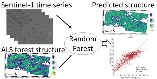
2.5. Structure Prediction Model

The structure metric derivation from S-1 time series was built around an RF-model [92], which took the 36 S-1 parameters (Table 1) as predictors and the ALS structure metrics as target variables. An RF-model was chosen, as it constitutes a non-parametric approach, i.e. does not make assumptions about the underlying statistic distributions of the variables. This is of special importance considering the different SAR-derived predictor variables. Furthermore, previous studies have shown the robustness and efficiency of the RF algorithm in comparison to other machine learning methods for mapping forest-related parameters (e.g., [47,93]).

Ascending and descending orbits were treated separately to this point and the time series metrics computed from the respective orbits are used as individual predictors in the model. An individual RF regression model was trained for each of the structure metrics and for each resolution. In case of the stand height, this also applied to the different aggregation modes.

The prediction models rely on the ranger-implementation of the RF framework [94] in R [90]. The performance of the RF-models is controlled by the number of trees (num.trees), which are established during the training phase and which form the assemblage of the random forest, and the number of variables (mtry), which are randomly selected for splitting at each node [94]. The values for these two parameters were previously tuned on a randomly selected 7 ha subset of the scene, where num.trees was varied in range [30, 300] and mtry in range [1, 14]. The accordance of the predictions with the actual measurements was highest for mtry = 6, while the increase of the model prediction performance beyond num.trees = 150 was little, for which reason we selected this parameterization. mtry = 6 is equivalent to the default parameter as estimated by ranger, corresponding to the rounded-down square root of the number of prediction variables.

2.6. Experimental Design

We conducted four experiments in our study. In a first experiment, we investigated which of the four aggregation modes for the stand height computation (i.e., the nDSM height aggregated as mean, or as 50%-, 75%- or 95%-height quantile of the nDSM height) can be best estimated from S-1 time series, and on which aggregation level (20 m, 40 m, 100 m) the predicted structure metrics showed the highest correspondence to the reference. The training samples were randomly selected from the entire set of forest pixels and no particular strategy was applied for the training of the RF-model.

In a second experiment, we focused on the aggregation level, and in case of the stand height the aggregation mode, for which we obtained the best results in the first experiment. For the respective settings, we then investigated improvements in the training phase of the RF-model through a stratified selection of training samples. Therefore, we stratified the training set into three and four classes, respectively. For the stand height prediction, we split the height range of 0–45 m, which is covered by the ALS heights, into groups with equal height intervals (i.e., 0–15 m, 15–30 m and >30 m) for the stratification into three groups, and into groups with intervals of 10 m (i.e., 0–10 m, 10–20 m, 20–30 m, and >30 m) for the stratification into four groups. For the fractional cover, the thresholds were set at 0.5 and 0.75 for the delineation of three classes, and to 0.5, 0.67 and 0.84 for four classes, respectively. From each stratified group, the same number of samples was randomly chosen, whereby the smallest stratification group defined the number of samples. For the mean height at 100 m resolution, this were 803 samples per class in case of three classes, and 744 samples per class in case of four classes. For the fractional cover at 100 m resolution, the class with coverages $\le 0.5$ was the smallest one, comprising 350 samples. Finally, in order to analyze the effect of the stratified training strategy, we reduced the training set from the non-stratified training set and the training set with the four stratified groups to the training sample size with three stratified groups, which was the smallest training set, through random sampling of the initially designated training sets.

The aim of the third experiment was to analyze the predictive power of the coherence metrics for the estimation of the forest structure. The experiment was carried out on a random, non-stratified selection of training samples, whereby we excluded the coherence metrics from the model.

In a final experiment, the transferability of the model to other years was tested. Therefore, we trained an RF-model using the 2018 data and applied it to S-1 time series metrics from 2017 and from 2019, which were processed in the same manner as the metrics for 2018, in order to estimate the stand height of these respective years.

In all experiments, the performance of the RF-models were evaluated in their spatial context through a visual inspection, and through a statistical analysis. In the first three experiments, we removed four 1.2 × 1.2 km${}^2$ tiles of the entire scene (red squares in Figure 1) previous to the separation of the training set and the test set, respectively, and the analysis of the spatial performance was then conducted on these tiles. In the fourth experiment, the exclusion of these tiles was not necessary because the models were transferred to data sets of different years, for which the spatial performance was then tested.

The statistics for the analysis in experiments 1 through 3 were computed from the joint pixel sets comprising of the designated test sample and the tile pixels. The test sample thereby was randomly drawn from the forest pixels. Yet, slightly different fractions of the forest pixels were picked as training and test samples in the three experiments after removal of the tiles (

Table 2. Fraction of pixels from the 2018 scene used for the training of the RF-models. The fraction refers to the number of pixels after four 1.2 × 1.2 km${}^2$ tiles have been removed from the scene, if they have been previously excluded. Only forest pixels were considered.

Experiment	Fraction for Training	Removed Tiles
1	75%	yes
2	80%	yes
3	75%	yes
4	100%	no

), as the design of the study reduced the number of potential training samples in case of the stratified training strategy.

We selected three measures describing the quality of the RF-model for the statistical analysis, namely the bias, the root mean square error (RMSE) and the correlation R between the reference and the predicted metrics. As ideally, the correlation between the reference and the prediction should be linear, we chose Pearson’s linear correlation coefficient as metrics for the latter, while bias and RMSE were computed as:

$$bias=\frac{1}{n}\sum _{i=1}^n\left(Predictio{n}_{S1}-Referenc{e}_{ALS}\right)$$

(3)

and

$$RMSE=\sqrt{\frac{{\sum }_{i=1}^n{\left(Predictio{n}_{S1}-Referenc{e}_{ALS}\right)}^2}{n}}$$

(4)

whereby n corresponds to the number of pixels in the test set, Prediction${}_{S1}$ to the forest metrics predicted by the RF-model, and Reference${}_{ALS}$ to the forest metrics computed from the ALS data set.

3. Results

3.1. ALS Metrics Aggregation

Figure 4 shows the maps of the aggregated ALS metrics mean stand height and fractional cover, respectively, both aggregated on cells with 100 m × 100 m extent, and cut to forested areas considering the forest mask. Products aggregated in this manner served as basis for the training and evaluation of the RF-models. The number of cells before and after the limitation to forested areas is depicted in

Table 3. Number of cells with valid forest metrics computed from the ALS data set before (all) and after the limitation to forested areas (forested).

Resolution	Number of Cells
	All	Forested
20 m	264,103	234,819
40 m	66,334	59,999
100 m	10,771	10,071

.

The mean stand height in the 100 m raster is 17.8 m with a maximum stand height of 42.9 m, while the fractional cover on 100 m has a mean of 0.76 and a median of 0.86. The histograms in Figure 6c,d give a clearer picture of the ALS metrics distributions within the test site.

3.2. Prediction of ALS Metrics

3.2.1. Stand Height

Figure 5 reports the bias, RMSE and Pearson’s R of the stand height predictions for the different aggregation levels (20, 40 and 100 m) and statistics with which the nDSM heights were aggregated (i.e., mean, and 50%-, 75%-, and 95%-quantile height, respectively). The bias changed from a slight underestimation of the predicted stand height on a 20 m aggregation level (−0.14 to −0.01 m) to an overestimation in the same range (≤0.11 m) on the 100 m aggregation level. RMSE decreased with increasing aggregation level (6.45 m to 7.07 m on 20 m, 5.83 m to 6.66 m on 40 m, 4.76 m to 5.91 m on 100 m), while the correlation between the reference and the prediction increases (0.74 to 0.79 on 20 m, 0.76 to 0.81 on 40 m, 0.79 to 0.88 on 100 m).

The observed biases for all modes on the same aggregation level were similar, while the RMSE was lower when the nDSM height was aggregated as mean height (down to 4.76 m on 100 m) than for aggregations deploying quantiles. Likewise, the correlation of the prediction to the reference was highest when using the mean value for aggregation.

Figure 6a,c depict a comparison of the mean ALS stand height, aggregated to 100 m (i.e., the best model, considering the performance metrics in Figure 5), to the respective prediction from S-1 time series. The scatter plot (Figure 6a) reveals a high correlation of the predicted stand heights to the reference (R = 0.88). Yet, the model showed a tendency to overestimate the height of smaller stand heights, while the heights of taller stands were underestimated. The histogram in Figure 6c illustrates this finding, showing a clear overestimation of predicted stand heights in the range of 20 m to 25 m, while the number of pixels with lower heights, and taller stands in particular, were under-represented in the prediction (Figure 6).

The maps of the predicted mean stand heights on 100 m (Figure 7 and Figure 8) reveal that the general height structure is reproduced well from S-1. Yet, the underestimation of taller stands, which we observed in Figure 6, can also be recognized in the maps and in the profile sampled from Tile 4 (Figure 9). Furthermore, while spatially distinct transitions in the stand height and gaps, in particular, stand out clearly in the prediction maps, it becomes apparent that small height variations are not represented well in the predictions.

3.2.2. Fractional Cover

The prediction of the fractional cover shows the highest agreement to the reference on a 100 m resolution. The distribution of the predicted covers corresponds well to the reference with a Pearsons’s R of 0.94 (Figure 6b), a bias of 0.0 and an RMSE of 0.08 (

Table 4. Performance of RF-models for the prediction of the fractional cover. Best scores for each measure are written in bolt letters.

	Bias	RMSE	Person’s R
20 m	−0.001	0.12	0.84
40 m	−0.001	0.10	0.89
100 m	0.000	0.08	0.94

). Yet, the comparison of the single predicted values (Figure 6d) reveals an over-representation of stands with fractional cover values in the range of 0.85 to 0.9, while in contrast, the model shows deficiencies in the detection of fractional cover values > 0.9.

The maps with the reconstructed tiles (Figure 10, and Figure A1 and Figure A2 (Appendix A)) showed that the patterns of the predicted fractional cover closely matched the fractional cover from the ALS reference, except for the mentioned deficiency to capture very dense stand coverages (e.g., south-eastern corner in Tile 3, Figure 10).

3.3. Stratified Training Sets

3.3.1. Stand Height

The distribution of the height values was non-uniform, but showed an over- representation of samples in the height class between 15 m and 30 m. In a second experiment, we therefore tested the effect of a stratified selection of training samples for the prediction of the mean stand height at 100 m resolution. The prediction performances of the RF-models without a stratified training set selection, and from the sets using three and four stratification groups, respectively, are shown in Figure 11 and summarized in

Table 5. Prediction error within the three height classes 0 m–15 m (H1), 15 m–30 m (H2), and >30 m (H3), respectively, for the RF-model trained with a non-stratified training set, and sets comprising of three and four height classes, respectively. Further stated are the overall Bias and RMSE measures for the three models. All measures are in [m].

	Non-Stratified			3 Classes			4 Classes
	H1	H2	H3	H1	H2	H3	H1	H2	H3
Bias	4.3	−0.7	−6.1	3.9	0.2	−3.8	3.6	-0.4	−4.7
RMSE	6.2	4.1	6.7	6.3	4.7	4.9	5.9	4.5	5.7
Bias${}_{tot}$	0.2			0.9			0.3
RMSE${}_{tot}$	5.1			5.2			5.1

. Overall, the error in the predicted heights was in the same range if stratified training sets were deployed (bias = 0.9 m, RMSE = 5.2 m for three classes; bias = 0.3 m, RMSE = 5.1 m for four classes) as if the training set was obtained through random sampling (bias = 0.2 m, RMSE = 5.1 m). Yet, the tendency to underestimate tall stand heights could be reduced. While the RF-model from the non-stratified training set showed a bias = $-6.1$ m and an RMSE = 6.7 m for stand heights > 30 m, the discrepancies to the reference in this height class were smaller if stratified training sets are used (bias = $-3.8$ m, RMSE = $4.9$ m for the model with three stratified groups; bias = $-4.7$ m, RMSE = $5.7$ m for the model with four stratified groups). Likewise, the histograms in Figure 11d–f illustrate the stratified models’ ability to also better reproduce stand heights below 15 m. While the bias was 4.3 m with an RMSE of 6.2 m for the non-stratified model, the bias was reduced to 3.9 and 3.6 m using three and four height classes in the stratified training set retrieval. Yet, the RMSE remained in the same range as for the non-stratified training set (RMSE = 6.3 m and 5.9 m for three and four stratification groups, respectively).

3.3.2. Fractional Cover

As for the stand height, the training sets for the RF-models for the prediction of the fractional cover were also obtained from subsets stratified into three and four cover classes, respectively, in a second experiment. Figure 12a–c compare the predicted fractional cover estimates at 100 m from the non-stratified training set (a), and for training sets stratified into three (b) and four (c) cover classes, respectively, to the reference. The statistics stated the errors of the RF-models to be similar, regardless of the deployed stratification strategy (RMSE = $0.08-0.09$), but to underestimate the fractional cover if stratified training sets were applied (bias = $-0.04$ and $-0.03$ for three and four stratification classes, respectively) in contrast to a bias of 0.0 in case of a non-stratified training set. Yet, the histograms in Figure 12d–f, where the predicted fractional cover values are compared to the ALS references, revealed that the models with stratified training sets could mitigate the over-representation of fractional cover values in the range 0.85 to around 0.9, but at the expense of lower fractional covers, which are now over-represented. The recognition of very dense plots, i.e., with fractional cover values > 0.95, however, was not improved through the stratification strategy.

3.4. Predictive Power of Coherence

The predictive power of the model for the mean stand height on 100 m deteriorates, if the coherence metrics are excluded (bias = 0.21 m, RMSE = 5.64 m) compared to the model including these metrics (bias = 0.09 m, RMSE = 4.76 m, cf. Figure 5). Low growing stands with heights < 15 m and tall stands with heights > 30 m are overestimated (bias = 5.8 m, RMSE = 7.2 m) and underestimated (bias = 7.3 m, RMSE = 8.0 m), respectively. Deficiencies in accurately estimating these height layers already occurred in the model including the coherence (Table 5), yet are more pronounced if the coherence is excluded. In particular, the predicted stand heights show a distinct break pointing towards an underestimation with increasing stand heights when the coherence metrics are excluded (Figure 13b) than when including coherence (Figure 6a). As a result, we can observe an over-representation of predicted medium stand heights for the model excluding coherence (Figure 13c), yet with a shift of the dominant over-represented height range to 15 m to 20 m, compared to the former model, which predominantly over-represents heights between 20 m and 25 m (Section 3.2.1, Figure 13a).

In case of the fractional cover, we can observe an increase of the error (RMSE = 0.08 vs. 0.11 for the model including and excluding coherence, respectively) and a decrease of the correlation (Pearson’s R = 0.94 vs. 0.82) if the coherence is excluded from the model. Yet, the histogram of the predicted values including (Figure 13d) and excluding the coherence (Figure 13f) reveals that coverages of forest stands with fractional covers larger 0.85 are more often underestimated if the coherence is excluded from the model than is the case including the coherence. In contrast, fractional covers in range 0.7 to 0.85 are more severely over-represented. As in the case of stand height, the tendency of the model to underestimate high vegetation densities is thus increased if the coherence is excluded (Figure 13).

3.5. Model Transfer

In a final experiment, we applied the model for stand height prediction from 2018 to S-1 time series acquired in 2017 and 2019. The estimated heights for 2017 and 2019 corresponded well (Pearson’s R = 0.89; Figure A3b (Appendix B)), and the spatial patterns of the predicted stand heights showed similar structures for both years (Figure A4 and Figure A5). However, the predicted stand height is higher for 2017 (mean stand height = 17.6 m) than for 2019 (mean stand height = 16.5 m, Figure A3a,c) and, consequently, the difference map (Figure A6) shows predominantly small negative changes for the 2 year time interval.

To verify our results, we analyzed whether major decreases in the predicted forest stand heights could be linked to observations in aerial images, as no point clouds were available to build the same type of reference data as in the experiments of Section 3.2, Section 3.3 and Section 3.4. We disregarded small height changes between 2017 and 2019 and focused on height decreases greater than 10 m. We subsequently compared the respective spots from the difference map to aerial photographs, where changes are recognizable. Figure 14 illustrates two exemplary plots with distinct negative height changes between the two investigated years. For cells with detected height decreases of more than 10 m between the investigated years, changes in the forest structure can be recognized in the aerial photographs. Note that the undetected gap in the second example, which is clearly visible in the south-west corner, to our knowledge was cleared in 2020.

4. Discussion

4.1. Prediction of Stand Height

Our results have shown that from the investigated aggregation levels, the correspondence of the predicted height from S-1 time series to the ALS reference is highest if the height is aggregated as mean nDSM height within 100 m cells. While biases for all models were close to 0 m, the overall prediction error in terms of the RMSE was smaller for this aggregation mode than the errors when using quantiles (Figure 5). The effect of the aggregation level was such that the bias and the RMSE decreased with increasing aggregation level from 20 to 100 m for the same aggregation mode. The model was able to reproduce the general forest height structure (Figure 7), however, we observed a saturation of the predicted stand heights for heights larger 25–30 m, which are systematically underestimated. This finding is in correspondence to other studies which reported the SAR backscatter to saturate with increasing biomass [95,96,97]. The accurate estimation of taller stands from SAR backscatter information is a pending task (e.g., [40]). Since the RF methodology is a non-linear, non-parametric model, known SAR backscatter dependencies on the forest structure are not considered explicitly by our RF-model. This may further affect the stand height prediction. SAR scattering models describing the SAR backscatter and phase in dependence of the forest volume (e.g., [39,40,43]), are advantageous in this respect since process understanding on scattering mechanisms can be incorporated into these models. The cited studies demonstrated that estimation errors could be kept small with such models.

In our study, we addressed the deficiency of the RF-model in the prediction of both tall and lower-height stands by applying a stratified sampling strategy for the selection of the training set. The correspondence of the predicted heights to the reference could be increased if random sub-samples of equal size were drawn from three or four stratified height classes for the training of the model (Figure 11a–c). In particular, the representation of the range of the heights within the test site could be improved through a stratified training set selection (Figure 11d–f). The improvement is reflected in the bias and RMSE of the investigated height classes (i.e., 0–15 m, 15–30 m, >30 m), whereas the prediction accuracy of the tallest of these height classes increased most noticeably (Table 5). Yet, in our experiment, the stratification into three classes yielded slightly better results than if four classes were distinguished. Therefore, three classes should be the better choice, also since the model is not tailored too specifically to one test site.

Studies using spaceborne sensors emphasize that the X-band, whose radiation is scattered on the uppermost canopy layers, offers the best canopy height prediction capability (e.g., RMSE in range of 2.6 m on a 31 × 15 m${}^2$ grid when using data from the Shuttle Radar Topography Mission (SRTM) [42]; RMSE in range 3.5 m to 4.3 m on a 90 m raster when using TanDEM-X data [98]) while predictions from L-band typically are lower (e.g., RMSE of 3–4 m on a grid size of 3–6 ha when using ALOS/PALSAR data [40]). The acquisition geometry of the TanDEM-X mission with its two sensor, small baseline constellation is therefore a valuable data source for forest structure derivation using SAR scattering models [63,64,65,66]. In contrast, SAR C-band in combination with an RF-model in our study delivered height predictions with slightly larger errors.

However, due to the increasing number of EO missions which provide freely accessible data and convenient access, these new spaceborne missions have gained interest, in particular the Sentinel-1 constellation. Yet, the sensor constellation of S-1 only allows for multi-pass interferometry, which, however, has a decreased coherence over vegetation [53], and does not allow for the derivation of the forest height using SAR scattering models. New approaches are therefore required for the derivation of forest structure information. Morin [46] and Li [47] demonstrated that machine learning frameworks are feasible means for the exploitation of open access, multi-modal EO data and that through this combination, similar estimation accuracies can be achieved as when using interferometric SAR in combination with scattering model inversion approaches. The results from our study showcase that such estimation accuracies can also be achieved from S-1 time series metrics alone, when introduced into a machine learning framework.

4.2. Prediction of Fractional Cover

As for the stand height, the best correspondence of the predicted fractional cover to the reference was achieved on a 100 m aggregation level (Table 4). Yet, here again, a saturation in the predicted values is discernible since the RF-model showed deficiencies in the prediction of fractional cover values above 0.9. Nevertheless, the RF-model was able to adequately reproduce the general density patterns (Figure 10), whereby distinct transitions were well retained and gaps, in particular, could be reproduced.

A stratified approach for the selection of the training samples lead to a less distinct improvement of the predictions than was the case for the stand height. Although the over-representation of predicted pixels in the range between 0.85 and 0.9 could be mitigated, the stratified training phase lead to an overestimation of lower fractional cover values, while the inability to recognize very dense stands remained.

One general issue with our study design is the fractional cover distribution within our test site, which shows a distinct left skewed density distribution with a mean fractional cover value of 0.79 and only 10% of the pixels having fractional cover values below 0.5. Studies by Lucas [45] and Urban [50], which investigated the potential to estimate the foliage cover and the woody cover, respectively, from SAR data, were performed over larger areas and over differing bioms to ours, covering a wider range of coverage densities. However, our test area corresponds to a typical temperate forest in Central Europe, which is why methods are required to capture such canopy densities.

4.3. Predictive Power of Coherence

One issue with the applied SAR metrics is the additional computation step which is required to estimate coherence. Applications of stand metrics estimations from S-1 time series would benefit if the coherence could be excluded from the models. We therefore tested the influence of the coherence in the RF-models for the prediction of the mean stand height and the fractional cover, both on a 100 m aggregation level. RF-models including and excluding the coherence metrics were applied on the same subset of test pixels in order to ensure their comparability.

The comparison of the prediction models including and excluding coherence metrics showed that the dynamic range in the stand height was better reproduced if the coherence was included in the model. The height overestimation of low-growing vegetation (i.e., stand heights < 15 m) was more severe if coherence was excluded from the model. For forest stands with heights > 30 m, the differences were less distinct since both models underestimated high-growing forest areas. Yet, the flattening tendency of height estimations with increasing stand height was more pronounced if the coherence was excluded (Figure 13b) when compared to the model including the coherence (Figure 6a), since already heights above 15 m were affected. In contrast, in the predictions including the coherence, a systematic underestimation applied to heights above 20 m only.

In the case of fractional cover, we could observe an increase in the error and a tendency of the model to over-represent fractional covers in the range 0.7 to 0.85 (Figure 13d,f), if the coherence was excluded from the model. Thus, here again, a clear improvement of the prediction accuracies could be attained when coherence was included.

Previous studies have investigated the relationship between biomass-related parameters and coherence and demonstrated the potential of coherence for the retrieval of biomass-related parameters (e.g., [77,78,79]). Generally, a lower multi-pass coherence was observed for higher biomass [53], in particular over forests [99,100,101]. The sensitivity of coherence to both, the stand height and the fractional cover, which we observed, is therefore consistent with the aforementioned studies and we consider the inclusion of coherence metrics in our RF-model as important.

4.4. Model Transfer

S-1 time series in combination with an RF-model offer the potential to update forest structure descriptions in annual intervals, thereby closing gaps between the ALS acquisitions. Following this intention, we applied a model from 2018 to predict stand heights for 2019 and 2017. The comparison of the predicted stand heights with the reference stand height from 2018 showed a similar pattern (Figure A3a,c) as we have observed in the model validation (Figure 6a), with a distinct saturation of the predicted height with increasing actual stand height. Likewise, the spatial analysis revealed a similar pattern of the predicted forest height structure for both years (Figure A4 and Figure A5) but also in comparison with 2018. Yet, the predicted stand height was larger for 2017 than for 2019. Although changes of the forest structure between 2017 and 2018, and between 2018 and 2019, respectively, should be similar, the height predictions for 2017 showed a higher correspondence to the 2018 reference (R = 0.81) than the prediction for 2019 (R = 0.75). However, the correspondence of the predictions for 2017 and 2019 was high (R = 0.89, Figure A3b). This supports our hypothesis that the model can in principle be applied to different years in order to derive updated information on the stand height, which is an important parameter in fire risk assessments as it is related to biomass and forest fuel [18,19,20].

From the stand height estimations derived in this manner, inter-annual changes in forest cover could be detected by applying a threshold of 10 m, corresponding to the minimum height decrease between 2017 and 2019. Within our test site comprising of managed forests, clearings originate from logging activities and predominantly affect mature forest stands, which are characterized by large heights. New clearings, therefore, should be clearly discernible since a change from a tall stand to nearly ground level can be detected. Information on newly emerging clearings are elementary for fire risk assessments as they represent locations which can act as potential fire ignition spots and need to be integrated into risk assessments. S-1 time series therefore are valuable to regularly update the forest structure information between ALS surveys over such managed forests, even if the accuracy of the predicted forest structure is not as high as from ALS data. Yet, based on our data set, we could not test the feasibility of our approach to detect major changes in non-managed, more natural forests.

The potential to recognize forest structure changes using S-1 time series has been reported in previous studies (e.g., [102]) and the detection of deforestation from S-1 data has been shown, whereby time series were applied [103,104] or the SAR shadowing effect was exploited [105]. These studies also highlight the potential of S-1 data for the detection of natural disturbances and of illegal logging activities, which, apart from fires, are crucial aspects in forest management. As becomes obvious from these studies, however, the detection of forest gaps and deforestation is a non-trivial task. We did not aim at providing such a thorough framework, but used the detection of large gaps, which we could identify in aerial images, as a way to test the transferability of the model, since we could not validate the models with reference data from the respective years.

The inter-annual transfer, however, also revealed some open issues of our method. The model prediction is based on the seasonal backscatter behaviour. Yet, the backscatter processes are not only controlled by the actual forest structure, but also by meteorological conditions. The impact of the temperature on the measured backscatter has been reported in previous studies [36,106,107]. Furthermore, the temperature controls the plant phenology in spring, which leads to differences in the S-1 time series across the years. Therefore, S-1 time series are more suitable for detecting larger forest structure changes on time scales of multiple years rather than inter-annual changes, since the reported prediction error (RMSE = 4.76 m, Figure 5) is larger than the yearly height increase.

Finally, the performance over different forest types, i.e., over conifer, deciduous or mixed forest stands, has to be investigated further. Rüetschi [36] and Dostálová [35] noted a distinct, opposing intra-annual backscatter pattern for deciduous and coniferous stands. Therefore, it should be tested whether the structure estimation works better for one of these specific forest types and even more so the requirement to train specific RF-models for each stand type. The required forest type maps for the stratification could be derived from S-1 time series in a preceding step, as these two studies further demonstrated. However, we could not perform a robust stratified analysis based on our data set as, firstly, only a small fraction of the test site was covered with conifer tree stands and secondly, the majority of these conifer stand pixels had stand heights below 10 m, and are thereby in the range of the largest prediction error (Table 5).

5. Conclusions

We tested the potential of S-1 time series for the derivation of forest stand height and fractional cover over a temperate deciduous forest area. Deriving vegetation structure parameters from S-1 would allow updating forest structure information on a yearly basis. This can augment ALS time series, which typically have multiple years between subsequent acquisitions.

Reference data derived from ALS was used to train a Random Forest model to estimate the vegetation structure. The comparison of the predictions of the RF-model to the ALS reference on different scales revealed the highest level of agreement at a 100 m resolution. The predicted mean stand height had an RMSE of 4.76 m (bias = 0.09 m; R = 0.88), while for the fractional cover the RMSE was 0.08 (bias = 0.0; R = 0.94). The comparison of the spatial arrangement of the structure metrics predictions to the reference showed that the general height and density structure, respectively, could be reproduced well by the RF-model. Yet, we recognized the predictions of both, stand height and fractional cover, to get into saturation. Stand heights above 30 m were underestimated as were dense stands with fractional cover values larger 0.9. Likewise, in case of the stand height, we recognized a deficit of the RF-model to accurately predict stand heights below 15 m, as the height of such low-growing stands were generally overestimated. The stratified selection of the training set, yielding a homogeneous distribution of the structure metrics for training, could partially mitigate but not completely eliminate the saturation behaviour. We further learned that the SAR coherence, which was evaluated as predictor in our model, was indeed crucial for the prediction accuracy, as its inclusion reduced the saturation tendency.

We further applied the trained RF-model to S-1 time series one year before and after the year, for which the model was trained. The predicted height values for the two years revealed a high level of consistency (R = 0.89), and the spatial patterns of the height predictions were similar, additionally confirming the effectiveness of our approach. Yet, the predicted heights of the earlier year were higher than those of the later (difference of the mean heights = 1.1 m).

Overall, the prediction accuracies in our experiments were close to those of previous studies, which predicted stand heights through the application of scattering model inversion on SAR interferometric data. We therefore conclude that S-1 time series in combination with machine learning frameworks facilitate the derivation of forest height and fractional cover. However, the approach should also be tested over coniferous and mixed forest stands, what was not possible in our study as the test site comprised predominantly deciduous tree species. This would further refine the approach and make it applicable for forest structure estimations over larger areas.

References

1. Chuvieco, E.; Yue, C.; Heil, A.; Mouillot, F.; Alonso-Canas, I.; Padilla, M.; Pereira, J.M.; Oom, D.; Tansey, K. A new global burned area product for climate assessment of fire impacts. Glob. Ecol. Biogeogr. 2016, 25, 619–629. [Google Scholar] [CrossRef] [Green Version]
2. Giglio, L.; Randerson, J.T.; Van Der Werf, G.R. Analysis of daily, monthly, and annual burned area using the fourth-generation global fire emissions database (GFED4). J. Geophys. Res. Biogeosci. 2013, 118, 317–328. [Google Scholar] [CrossRef] [Green Version]
3. Kasischke, E.S.; Bruhwiler, L.P. Emissions of carbon dioxide, carbon monoxide, and methane from boreal forest fires in 1998. J. Geophys. Res. Atmos. 2002, 107, FFR2-1–FFR2-14. [Google Scholar] [CrossRef] [Green Version]
4. Van der Werf, G.R.; Randerson, J.T.; Giglio, L.; Collatz, G.; Mu, M.; Kasibhatla, P.S.; Morton, D.C.; DeFries, R.; Jin, Y.; van Leeuwen, T.T. Global fire emissions and the contribution of deforestation, savanna, forest, agricultural, and peat fires (1997–2009). Atmos. Chem. Phys. 2010, 10, 11707–11735. [Google Scholar] [CrossRef] [Green Version]
5. Vinogradova, A.; Smirnov, N.; Korotkov, V.; Romanovskaya, A. Forest fires in Siberia and the Far East: Emissions and atmospheric transport of black carbon to the Arctic. Atmos. Ocean. Opt. 2015, 28, 566–574. [Google Scholar] [CrossRef]
6. Langenfelds, R.; Francey, R.; Pak, B.; Steele, L.; Lloyd, J.; Trudinger, C.; Allison, C. Interannual growth rate variations of atmospheric CO2 and its δ13C, H2, CH4, and CO between 1992 and 1999 linked to biomass burning. Glob. Biogeochem. Cycles 2002, 16, 21-1–21-22. [Google Scholar] [CrossRef]
7. Simpson, I.J.; Rowland, F.S.; Meinardi, S.; Blake, D.R. Influence of biomass burning during recent fluctuations in the slow growth of global tropospheric methane. Geophys. Res. Lett. 2006, 33. [Google Scholar] [CrossRef] [Green Version]
8. Abatzoglou, J.T.; Williams, A.P. Impact of anthropogenic climate change on wildfire across western US forests. Proc. Natl. Acad. Sci. USA 2016, 113, 11770–11775. [Google Scholar] [CrossRef] [Green Version]
9. Müller, M.M.; Vilà-Vilardell, L.; Vacik, H. Towards an integrated forest fire danger assessment system for the European Alps. Ecol. Inform. 2020, 60, 101151. [Google Scholar] [CrossRef]
10. Wastl, C.; Schunk, C.; Lüpke, M.; Cocca, G.; Conedera, M.; Valese, E.; Menzel, A. Large-scale weather types, forest fire danger, and wildfire occurrence in the Alps. Agric. For. Meteorol. 2013, 168, 15–25. [Google Scholar] [CrossRef]
11. Müller, M.M.; Vacik, H.; Valese, E. Anomalies of the Austrian forest fire regime in comparison with other Alpine countries: A research note. Forests 2015, 6, 903–913. [Google Scholar] [CrossRef]
12. Arpaci, A.; Eastaugh, C.S.; Vacik, H. Selecting the best performing fire weather indices for Austrian ecoregions. Theor. Appl. Climatol. 2013, 114, 393–406. [Google Scholar] [CrossRef] [PubMed] [Green Version]
13. Jolly, W.M.; Cochrane, M.A.; Freeborn, P.H.; Holden, Z.A.; Brown, T.J.; Williamson, G.J.; Bowman, D.M. Climate-induced variations in global wildfire danger from 1979 to 2013. Nat. Commun. 2015, 6, 1–11. [Google Scholar] [CrossRef]
14. Arpaci, A.; Malowerschnig, B.; Sass, O.; Vacik, H. Using multi variate data mining techniques for estimating fire susceptibility of Tyrolean forests. Appl. Geogr. 2014, 53, 258–270. [Google Scholar] [CrossRef]
15. Vacik, H.; Arndt, N.; Arpaci, A.; Koch, V.; Müller, M.; Gossow, H. Characterisation of forest fires in Austria. Austrian J. For. Sci. 2011, 128, 1–31. [Google Scholar]
16. Müller, M.M.; Vacik, H.; Diendorfer, G.; Arpaci, A.; Formayer, H.; Gossow, H. Analysis of lightning-induced forest fires in Austria. Theor. Appl. Climatol. 2013, 111, 183–193. [Google Scholar] [CrossRef] [Green Version]
17. Chuvieco, E.; Aguado, I.; Yebra, M.; Nieto, H.; Salas, J.; Martín, M.P.; Vilar, L.; Martínez, J.; Martín, S.; Ibarra, P.; et al. Development of a framework for fire risk assessment using remote sensing and geographic information system technologies. Ecol. Model. 2010, 221, 46–58. [Google Scholar] [CrossRef]
18. Chuvieco, E.; Allgöwer, B.; Salas, J. Integration of physical and human factors in fire danger assessment. In Wildland Fire Danger Estimation and Mapping: The Role of Remote Sensing Data; World Scientific: Singapore, 2003; pp. 197–218. [Google Scholar]
19. García, M.; Riaño, D.; Chuvieco, E.; Salas, J.; Danson, F.M. Multispectral and LiDAR data fusion for fuel type mapping using Support Vector Machine and decision rules. Remote Sens. Environ. 2011, 115, 1369–1379. [Google Scholar] [CrossRef]
20. Domingo, D.; de la Riva, J.; Lamelas, M.T.; García-Martín, A.; Ibarra, P.; Echeverría, M.; Hoffrén, R. Fuel Type Classification Using Airborne Laser Scanning and Sentinel 2 Data in Mediterranean Forest Affected by Wildfires. Remote Sens. 2020, 12, 3660. [Google Scholar] [CrossRef]
21. Holmgren, J.; Persson, Å. Identifying species of individual trees using airborne laser scanner. Remote Sens. Environ. 2004, 90, 415–423. [Google Scholar] [CrossRef]
22. Hollaus, M.; Mücke, W.; Höfle, B.; Dorigo, W.; Pfeifer, N.; Wagner, W.; Bauerhansl, C.; Regner, B. Tree species classification based on full-waveform airborne laser scanning data. In Proceedings of the SilviLaser, College Station, TX, USA, 14–16 October 2009. [Google Scholar]
23. Korpela, I.; Ørka, H.O.; Maltamo, M.; Tokola, T.; Hyyppä, J. Tree species classification using airborne LiDAR–effects of stand and tree parameters, downsizing of training set, intensity normalization, and sensor type. Silva Fenn. 2010, 44, 319–339. [Google Scholar] [CrossRef] [Green Version]
24. Hill, R.; Broughton, R.K. Mapping the understorey of deciduous woodland from leaf-on and leaf-off airborne LiDAR data: A case study in lowland Britain. ISPRS J. Photogramm. Remote Sens. 2009, 64, 223–233. [Google Scholar] [CrossRef]
25. Morsdorf, F.; Mårell, A.; Koetz, B.; Cassagne, N.; Pimont, F.; Rigolot, E.; Allgöwer, B. Discrimination of vegetation strata in a multi-layered Mediterranean forest ecosystem using height and intensity information derived from airborne laser scanning. Remote Sens. Environ. 2010, 114, 1403–1415. [Google Scholar] [CrossRef] [Green Version]
26. Leiterer, R.; Torabzadeh, H.; Furrer, R.; Schaepman, M.E.; Morsdorf, F. Towards automated characterization of canopy layering in mixed temperate forests using airborne laser scanning. Forests 2015, 6, 4146–4167. [Google Scholar] [CrossRef] [Green Version]
27. Crespo-Peremarch, P.; Tompalski, P.; Coops, N.C.; Ruiz, L.Á. Characterizing understory vegetation in Mediterranean forests using full-waveform airborne laser scanning data. Remote Sens. Environ. 2018, 217, 400–413. [Google Scholar] [CrossRef]
28. Maltamo, M.; Hyyppä, J.; Malinen, J. A comparative study of the use of laser scanner data and field measurements in the prediction of crown height in boreal forests. Scand. J. For. Res. 2006, 21, 231–238. [Google Scholar] [CrossRef]
29. Vauhkonen, J. Estimating crown base height for Scots pine by means of the 3D geometry of airborne laser scanning data. Int. J. Remote Sens. 2010, 31, 1213–1226. [Google Scholar] [CrossRef]
30. Popescu, S.C.; Zhao, K. A voxel-based lidar method for estimating crown base height for deciduous and pine trees. Remote Sens. Environ. 2008, 112, 767–781. [Google Scholar] [CrossRef]
31. Morsdorf, F.; Meier, E.; Kötz, B.; Itten, K.I.; Dobbertin, M.; Allgöwer, B. LIDAR-based geometric reconstruction of boreal type forest stands at single tree level for forest and wildland fire management. Remote Sens. Environ. 2004, 92, 353–362. [Google Scholar] [CrossRef]
32. Hollaus, M. 3D Point clouds for forestry applications. Österreichische Z. Vermess. Geoinf. VGI 2015, 103, 138–150. [Google Scholar]
33. Fisher, A.; Armston, J.; Goodwin, N.; Scarth, P. Modelling canopy gap probability, foliage projective cover and crown projective cover from airborne lidar metrics in Australian forests and woodlands. Remote Sens. Environ. 2020, 237, 111520. [Google Scholar] [CrossRef]
34. Kellndorfer, J.M.; Pierce, L.E.; Dobson, M.C.; Ulaby, F.T. Toward consistent regional-to-global-scale vegetation characterization using orbital SAR systems. IEEE Trans. Geosci. Remote Sens. 1998, 36, 1396–1411. [Google Scholar] [CrossRef]
35. Dostálová, A.; Wagner, W.; Milenković, M.; Hollaus, M. Annual seasonality in Sentinel-1 signal for forest mapping and forest type classification. Int. J. Remote Sens. 2018, 39, 7738–7760. [Google Scholar] [CrossRef]
36. Rüetschi, M.; Schaepman, M.E.; Small, D. Using multitemporal sentinel-1 c-band backscatter to monitor phenology and classify deciduous and coniferous forests in northern switzerland. Remote Sens. 2018, 10, 55. [Google Scholar] [CrossRef] [Green Version]
37. Kaasalainen, S.; Holopainen, M.; Karjalainen, M.; Vastaranta, M.; Kankare, V.; Karila, K.; Osmanoglu, B. Combining lidar and synthetic aperture radar data to estimate forest biomass: Status and prospects. Forests 2015, 6, 252–270. [Google Scholar] [CrossRef]
38. Kellndorfer, J.; Walker, W.; Pierce, L.; Dobson, C.; Fites, J.A.; Hunsaker, C.; Vona, J.; Clutter, M. Vegetation height estimation from shuttle radar topography mission and national elevation datasets. Remote Sens. Environ. 2004, 93, 339–358. [Google Scholar] [CrossRef]
39. Praks, J.; Antropov, O.; Hallikainen, M.T. LIDAR-aided SAR interferometry studies in boreal forest: Scattering phase center and extinction coefficient at X-and L-band. IEEE Trans. Geosci. Remote Sens. 2012, 50, 3831–3843. [Google Scholar] [CrossRef]
40. Lei, Y.; Siqueira, P.; Torbick, N.; Ducey, M.; Chowdhury, D.; Salas, W. Generation of Large-Scale Moderate-Resolution Forest Height Mosaic With Spaceborne Repeat-Pass SAR Interferometry and Lidar. IEEE Trans. Geosci. Remote Sens. 2019, 57, 770–787. [Google Scholar] [CrossRef]
41. Siqueira, P.; Hensley, S.; Chapman, B.; Ahmed, R. Combining lidar and InSAR observations over the harvard and duke forests for making wide area maps of vegetation height. In Proceedings of the IGARSS 2008—2008 IEEE International Geoscience and Remote Sensing Symposium, Boston, MA, USA, 7–11 July 2008; Volume 5, pp. 538–541. [Google Scholar] [CrossRef]
42. Solberg, S.; Astrup, R.; Bollandsås, O.M.; Næsset, E.; Weydahl, D.J. Deriving forest monitoring variables from X-band InSAR SRTM height. Can. J. Remote Sens. 2010, 36, 68–79. [Google Scholar] [CrossRef]
43. Soja, M.J.; Persson, H.; Ulander, L.M. Estimation of forest height and canopy density from a single InSAR correlation coefficient. IEEE Geosci. Remote Sens. Lett. 2014, 12, 646–650. [Google Scholar] [CrossRef] [Green Version]
44. Yu, X.; Hyyppä, J.; Karjalainen, M.; Nurminen, K.; Karila, K.; Vastaranta, M.; Kankare, V.; Kaartinen, H.; Holopainen, M.; Honkavaara, E.; et al. Comparison of laser and stereo optical, SAR and InSAR point clouds from air-and space-borne sources in the retrieval of forest inventory attributes. Remote Sens. 2015, 7, 15933–15954. [Google Scholar] [CrossRef] [Green Version]
45. Lucas, R.M.; Cronin, N.; Moghaddam, M.; Lee, A.; Armston, J.; Bunting, P.; Witte, C. Integration of radar and Landsat-derived foliage projected cover for woody regrowth mapping, Queensland, Australia. Remote Sens. Environ. 2006, 100, 388–406. [Google Scholar] [CrossRef] [Green Version]
46. Morin, D.; Planells, M.; Guyon, D.; Villard, L.; Mermoz, S.; Bouvet, A.; Thevenon, H.; Dejoux, J.F.; Le Toan, T.; Dedieu, G. Estimation and mapping of forest structure parameters from open access satellite images: Development of a generic method with a study case on coniferous plantation. Remote Sens. 2019, 11, 1275. [Google Scholar] [CrossRef] [Green Version]
47. Li, W.; Niu, Z.; Shang, R.; Qin, Y.; Wang, L.; Chen, H. High-resolution mapping of forest canopy height using machine learning by coupling ICESat-2 LiDAR with Sentinel-1, Sentinel-2 and Landsat-8 data. Int. J. Appl. Earth Obs. Geoinf. 2020, 92, 102163. [Google Scholar] [CrossRef]
48. Urbazaev, M.; Thiel, C.; Mathieu, R.; Naidoo, L.; Levick, S.R.; Smit, I.P.; Asner, G.P.; Schmullius, C. Assessment of the mapping of fractional woody cover in southern African savannas using multi-temporal and polarimetric ALOS PALSAR L-band images. Remote Sens. Environ. 2015, 166, 138–153. [Google Scholar] [CrossRef] [Green Version]
49. Dostálová, A.; Lang, M.; Ivanovs, J.; Waser, L.T.; Wagner, W. European Wide Forest Classification Based on Sentinel-1 Data. Remote Sens. 2021, 13, 337. [Google Scholar] [CrossRef]
50. Urban, M.; Heckel, K.; Berger, C.; Schratz, P.; Smit, I.P.; Strydom, T.; Baade, J.; Schmullius, C. Woody cover mapping in the savanna ecosystem of the Kruger National Park using Sentinel-1 C-Band time series data. Koedoe 2020, 62, 6. [Google Scholar] [CrossRef]
51. Torres, R.; Snoeij, P.; Geudtner, D.; Bibby, D.; Davidson, M.; Attema, E.; Potin, P.; Rommen, B.; Floury, N.; Brown, M.; et al. GMES Sentinel-1 mission. Remote Sens. Environ. 2012, 120, 9–24. [Google Scholar] [CrossRef]
52. Karjalainen, M.; Kankare, V.; Vastaranta, M.; Holopainen, M.; Hyyppä, J. Prediction of plot-level forest variables using TerraSAR-X stereo SAR data. Remote Sens. Environ. 2012, 117, 338–347. [Google Scholar] [CrossRef]
53. Solimini, D. Understanding Earth Observation; Springer International Publishing: Basel, Switzerland, 2016; pp. 1–703. [Google Scholar]
54. Erdody, T.L.; Moskal, L.M. Fusion of LiDAR and imagery for estimating forest canopy fuels. Remote Sens. Environ. 2010, 114, 725–737. [Google Scholar] [CrossRef]
55. Hermosilla, T.; Ruiz, L.A.; Kazakova, A.N.; Coops, N.C.; Moskal, L.M. Estimation of forest structure and canopy fuel parameters from small-footprint full-waveform LiDAR data. Int. J. Wildland Fire 2014, 23, 224–233. [Google Scholar] [CrossRef] [Green Version]
56. Jennings, S.; Brown, N.; Sheil, D. Assessing forest canopies and understorey illumination: Canopy closure, canopy cover and other measures. Forestry 1999, 72, 59–74. [Google Scholar] [CrossRef]
57. Korhonen, L.; Korpela, I.; Heiskanen, J.; Maltamo, M. Airborne discrete-return LIDAR data in the estimation of vertical canopy cover, angular canopy closure and leaf area index. Remote Sens. Environ. 2011, 115, 1065–1080. [Google Scholar] [CrossRef]
58. Jenkins, M.J.; Hebertson, E.; Page, W.; Jorgensen, C.A. Bark beetles, fuels, fires and implications for forest management in the Intermountain West. For. Ecol. Manag. 2008, 254, 16–34. [Google Scholar] [CrossRef]
59. Riaño, D.; Valladares, F.; Condés, S.; Chuvieco, E. Estimation of leaf area index and covered ground from airborne laser scanner (Lidar) in two contrasting forests. Agric. For. Meteorol. 2004, 124, 269–275. [Google Scholar] [CrossRef]
60. Morsdorf, F.; Kötz, B.; Meier, E.; Itten, K.; Allgöwer, B. Estimation of LAI and fractional cover from small footprint airborne laser scanning data based on gap fraction. Remote Sens. Environ. 2006, 104, 50–61. [Google Scholar] [CrossRef]
61. Solberg, S.; Næsset, E.; Hanssen, K.H.; Christiansen, E. Mapping defoliation during a severe insect attack on Scots pine using airborne laser scanning. Remote Sens. Environ. 2006, 102, 364–376. [Google Scholar] [CrossRef]
62. Holmgren, J.; Johansson, F.; Olofsson, K.; Olsson, H.; Glimskär, A. Estimation of crown coverage using airborne laser scanning. In Proceedings of the SilviLaser 2008, Scotland, UK, 17–19 September 2008; pp. 50–57. [Google Scholar]
63. Askne, J.I.; Fransson, J.E.; Santoro, M.; Soja, M.J.; Ulander, L.M. Model-based biomass estimation of a hemi-boreal forest from multitemporal TanDEM-X acquisitions. Remote Sens. 2013, 5, 5574–5597. [Google Scholar] [CrossRef] [Green Version]
64. Solberg, S.; Astrup, R.; Breidenbach, J.; Nilsen, B.; Weydahl, D. Monitoring spruce volume and biomass with InSAR data from TanDEM-X. Remote Sens. Environ. 2013, 139, 60–67. [Google Scholar] [CrossRef]
65. Kugler, F.; Schulze, D.; Hajnsek, I.; Pretzsch, H.; Papathanassiou, K.P. TanDEM-X Pol-InSAR performance for forest height estimation. IEEE Trans. Geosci. Remote Sens. 2014, 52, 6404–6422. [Google Scholar] [CrossRef]
66. Lee, S.K.; Fatoyinbo, T.E. TanDEM-X Pol-InSAR inversion for mangrove canopy height estimation. IEEE J. Sel. Top. Appl. Earth Obs. Remote Sens. 2015, 8, 3608–3618. [Google Scholar] [CrossRef]
67. Richards, J.A. Remote Sensing with Imaging Radar; Signals and Communication Technology; Springer: Berlin/Heidelberg, Germany, 2009; p. 361. [Google Scholar] [CrossRef]
68. Immitzer, M.; Neuwirth, M.; Böck, S.; Brenner, H.; Vuolo, F.; Atzberger, C. Optimal input features for tree species classification in Central Europe based on multi-temporal Sentinel-2 data. Remote Sens. 2019, 11, 2599. [Google Scholar] [CrossRef] [Green Version]
69. Lawrence, M.; McRoberts, R.E.; Tomppo, E.; Gschwantner, T.; Gabler, K. Comparisons of National Forest Inventories. In National Forest Inventories; Springer: Berlin/Heidelberg, Germany, 2010; pp. 19–32. [Google Scholar] [CrossRef]
70. RIEGL. VQ-1560i Datasheet; RIEGL Laser Measurement Systems GmbH: Horn, Austria, 2019. [Google Scholar]
71. Bauer-Marschallinger, B.; Sabel, D.; Wagner, W. Optimisation of global grids for high-resolution remote sensing data. Comput. Geosci. 2014, 72, 84–93. [Google Scholar] [CrossRef]
72. Pfeifer, N.; Mandlburger, G.; Otepka, J.; Karel, W. OPALS–A framework for Airborne Laser Scanning data analysis. Comput. Environ. Urban Syst. 2014, 45, 125–136. [Google Scholar] [CrossRef]
73. Hollaus, M.; Mandlburger, G.; Pfeifer, N.; Mücke, W. Land cover dependent derivation of digital surface models from airborne laser scanning data. In Proceedings of the ISPRS Commission III Symposium PCV 2010, IAPRS Volume XXXVIII Part 3A, Saint-Mandé, France, 1–3 September 2010; pp. 221–226. [Google Scholar]
74. Le Toan, T.; Beaudoin, A.; Riom, J.; Guyon, D. Relating forest biomass to SAR data. IEEE Trans. Geosci. Remote Sens. 1992, 30, 403–411. [Google Scholar] [CrossRef]
75. Ranson, K.; Sun, G. Mapping biomass of a northern forest using multifrequency SAR data. IEEE Trans. Geosci. Remote Sens. 1994, 32, 388–396. [Google Scholar] [CrossRef]
76. Vreugdenhil, M.; Wagner, W.; Bauer-Marschallinger, B.; Pfeil, I.; Teubner, I.; Rüdiger, C.; Strauss, P. Sensitivity of Sentinel-1 backscatter to vegetation dynamics: An Austrian case study. Remote Sens. 2018, 10, 1396. [Google Scholar] [CrossRef] [Green Version]
77. Santoro, M.; Shvidenko, A.; McCallum, I.; Askne, J.; Schmullius, C. Properties of ERS-1/2 coherence in the Siberian boreal forest and implications for stem volume retrieval. Remote Sens. Environ. 2007, 106, 154–172. [Google Scholar] [CrossRef]
78. Karila, K.; Vastaranta, M.; Karjalainen, M.; Kaasalainen, S. Tandem-X interferometry in the prediction of forest inventory attributes in managed boreal forests. Remote Sens. Environ. 2015, 159, 259–268. [Google Scholar] [CrossRef]
79. Persson, H.J.; Fransson, J.E. Comparison between TanDEM-X-and ALS-based estimation of aboveground biomass and tree height in boreal forests. Scand. J. For. Res. 2017, 32, 306–319. [Google Scholar] [CrossRef] [Green Version]
80. Dostálová, A.; Milenkovic, M.; Hollaus, M.; Wagner, W. Influence of Forest Structure on the Sentinel-1 Backscatter Variation-Analysis with Full-Waveform LiDAR Data. In Proceedings of the Living Planet Symposium, Prague, Czech Republic, 9–13 May 2016. [Google Scholar]
81. Small, D.; Miranda, N.; Ewen, T.; Jonas, T. Reliably flattened radar backscatter for wet snow mapping from wide-swath sensors. In Proceedings of the ESA Living Planet Symposium, Edinburgh, UK, 9–13 September 2013. [Google Scholar]
82. Atwood, D.K.; Small, D.; Gens, R. Improving PolSAR land cover classification with radiometric correction of the coherency matrix. IEEE J. Sel. Top. Appl. Earth Obs. Remote Sens. 2012, 5, 848–856. [Google Scholar] [CrossRef]
83. Small, D. Flattening gamma: Radiometric terrain correction for SAR imagery. IEEE Trans. Geosci. Remote Sens. 2011, 49, 3081–3093. [Google Scholar] [CrossRef]
84. Dostálová, A.; Hollaus, M.; Milenković, M.; Wagner, W. Forest area derivation from sentinel-1 data. ISPRS Ann. Photogramm. Remote Sens. Spat. Inf. Sci. 2016, 3, 227. [Google Scholar] [CrossRef] [Green Version]
85. ACube. Austrian Data Cube. An EODC Service for the Austrian Earth Observation User Community. Available online: https://acube.eodc.eu/ (accessed on 1 February 2021).
86. Naeimi, V.; Elefante, S.; Cao, S.; Wagner, W.; Dostalova, A.; Bauer-Marschallinger, B. Geophysical parameters retrieval from Sentinel-1 SAR data: A case study for high performance computing at EODC. In Proceedings of the 24th High Performance Computing Symposium, Pasadena, CA, USA, 3–6 April 2016; pp. 1–8. [Google Scholar]
87. SNAP. Sentinel Application Platform. Available online: https://step.esa.int/main/toolboxes/snap/ (accessed on 1 February 2021).
88. Geoland. Digitales Geländemodell (DGM) Österreich. 2020. Available online: https://www.data.gv.at/katalog/dataset/dgm (accessed on 1 February 2021).
89. Koskinen, J.T.; Pulliainen, J.T.; Hallikainen, M.T. The Use of ERS-1 SAR Data in Snow Melt Monitoring. IEEE Trans. Geosci. Remote Sens. 1997, 35, 601–610. [Google Scholar] [CrossRef]
90. R Core Team. R: A Language and Environment for Statistical Computing; R Foundation for Statistical Computing: Vienna, Austria, 2019. [Google Scholar]
91. Hijmans, R.J. Raster: Geographic Data Analysis and Modeling. R package version 3.3-13. 2020. Available online: https://CRAN.R-project.org/package=raste (accessed on 1 February 2021).
92. Breiman, L. Random forests. Mach. Learn. 2001, 45, 5–32. [Google Scholar] [CrossRef] [Green Version]
93. Latifi, H.; Koch, B. Evaluation of most similar neighbour and random forest methods for imputing forest inventory variables using data from target and auxiliary stands. Int. J. Remote Sens. 2012, 33, 6668–6694. [Google Scholar] [CrossRef]
94. Wright, M.N.; Ziegler, A. ranger: A Fast Implementation of Random Forests for High Dimensional Data in C++ and R. J. Stat. Softw. 2017, 77, 1–17. [Google Scholar] [CrossRef] [Green Version]
95. Lucas, R.M.; Cronin, N.; Lee, A.; Moghaddam, M.; Witte, C.; Tickle, P. Empirical relationships between AIRSAR backscatter and LiDAR-derived forest biomass, Queensland, Australia. Remote Sens. Environ. 2006, 100, 407–425. [Google Scholar] [CrossRef]
96. Cartus, O.; Santoro, M.; Kellndorfer, J. Mapping forest aboveground biomass in the Northeastern United States with ALOS PALSAR dual-polarization L-band. Remote Sens. Environ. 2012, 124, 466–478. [Google Scholar] [CrossRef]
97. Mermoz, S.; Le Toan, T.; Villard, L.; Réjou-Méchain, M.; Seifert-Granzin, J. Biomass assessment in the Cameroon savanna using ALOS PALSAR data. Remote Sens. Environ. 2014, 155, 109–119. [Google Scholar] [CrossRef]
98. Qi, W.; Dubayah, R.O. Combining Tandem-X InSAR and simulated GEDI lidar observations for forest structure mapping. Remote Sens. Environ. 2016, 187, 253–266. [Google Scholar] [CrossRef]
99. Hagberg, J.O.; Ulander, L.M.; Askne, J. Repeat-pass SAR interferometry over forested terrain. IEEE Trans. Geosci. Remote Sens. 1995, 33, 331–340. [Google Scholar] [CrossRef]
100. Askne, J.I.; Dammert, P.B.; Ulander, L.M.; Smith, G. C-band repeat-pass interferometric SAR observations of the forest. IEEE Trans. Geosci. Remote Sens. 1997, 35, 25–35. [Google Scholar] [CrossRef]
101. Wegmüller, U.; Werner, C. Retrieval of vegetation parameters with SAR interferometry. IEEE Trans. Geosci. Remote Sens. 1997, 35, 18–24. [Google Scholar] [CrossRef]
102. Rüetschi, M.; Small, D.; Waser, L.T. Rapid Detection of Windthrows using Sentinel-1 C-band SAR Data. Remote Sens. 2019, 11, 115. [Google Scholar] [CrossRef] [Green Version]
103. Lohberger, S.; Stängel, M.; Atwood, E.C.; Siegert, F. Spatial evaluation of Indonesia’s 2015 fire-affected area and estimated carbon emissions using Sentinel-1. Glob. Chang. Biol. 2018, 24, 644–654. [Google Scholar] [CrossRef] [PubMed]
104. Reiche, J.; Hamunyela, E.; Verbesselt, J.; Hoekman, D.; Herold, M. Improving near-real time deforestation monitoring in tropical dry forests by combining dense Sentinel-1 time series with Landsat and ALOS-2 PALSAR-2. Remote Sens. Environ. 2018, 204, 147–161. [Google Scholar] [CrossRef]
105. Bouvet, A.; Mermoz, S.; Ballère, M.; Koleck, T.; Le Toan, T. Use of the SAR shadowing effect for deforestation detection with Sentinel-1 time series. Remote Sens. 2018, 10, 1250. [Google Scholar] [CrossRef] [Green Version]
106. Way, J.; Paris, J.; Kasischke, E.; Slaughter, C.; Viereck, L.; Christensen, N.; Dobson, M.C.; Ulaby, F.; Richards, J.; Milne, A.; et al. The effect of changing environmental conditions on microwave signatures of forest ecosystems: Preliminary results of the March 1988 Alaskan aircraft SAR experiment. Int. J. Remote Sens. 1990, 11, 1119–1144. [Google Scholar] [CrossRef]
107. Olesk, A.; Voormansik, K.; Põhjala, M.; Noorma, M. Forest change detection from Sentinel-1 and ALOS-2 satellite images. In Proceedings of the 2015 IEEE 5th Asia-Pacific Conference on Synthetic Aperture Radar (APSAR), Singapore, 1–4 September 2015; pp. 522–527. [Google Scholar] [CrossRef]
Figure 1. Overview of Wienerwald test site. (Top): True color orthophoto (image source: Google Maps). The red squares mark four 1.2 × 1.2 km 2 tiles, which were used for the visual validation. (Bottom): 1 m normalized DSM derived from the ALS point cloud. Coordinates are in Equi7 Grid [71].
Remotesensing 13 00798 g001
Figure 2. Processing of the airborne laser scanning (ALS) data set, starting with a point cloud in Equi7 Grid coordinates [71].
Remotesensing 13 00798 g002
Figure 3. Processing of the S-1 data to derive radiometric terrain flattened Gamma Nought ( γ r t f ) backscatter and coherence.
Remotesensing 13 00798 g003
Figure 4. Maps of the aggregated ALS metrics, cut to forested areas. (Top) Stand height, aggregated to a 100 m raster, whereby each raster cell was assigned the mean height from the 1 m normalized digital surface model (nDSM). (Bottom) Fractional cover, computed for a 100 m raster grid. Coordinates are in Equi7 Grid [71].
Remotesensing 13 00798 g004aRemotesensing 13 00798 g004b
Figure 5. Bias (left), RMSE (middle) and correlation (right) of the stand heights predicted through RF-models, compared to the reference data. Depicted are the respective values for four different aggregation modes (mean, 50%-, 75%-, 95%-quantile of the nDSM) and for three resolutions (20 m, 40 m, 100 m).
Remotesensing 13 00798 g005
Figure 6. (ad) Comparison of the structure metrics predicted from S-1 time series to the reference values. Left column: stand height, aggregated as mean nDSM height, on 100 m aggregation level; right column: fractional cover on 100 m aggregation level. Top row: Relationship between the ALS reference (x-axis) and the RF-prediction (y-axis). Bottom row: histograms of the reference (white) and the predicted metrics (red).
Remotesensing 13 00798 g006
Figure 7. Maps of predicted mean nDSM height, aggregated on 100 m (top row) against the reference (second row). The third row shows the difference between the predicted and the reference stand height. The maps on the bottom depict the nDSM at 1 m resolution, which corresponds to the base product from which the aggregated ALS stand height was derived. The maximum color value for each scene was set to the maximum predicted height of the respective scene. White pixels depict non-forested areas.
Remotesensing 13 00798 g007
Figure 8. Predicted (left) versus reference mean stand height (right) on 100 m aggregation level for Tile 4. The map in the middle shows the respective nDSM at 1 m resolution. White pixels depict non-forested areas. The red lines mark the boarders of the profile in Figure 9.
Remotesensing 13 00798 g008
Figure 9. Profile from Tile 4, depicting the heights of the nDSM at 1 m resolution (gray dots). The profile width is 100 m, centered at 5,247,350 m east (red lines in the nDSM map Figure 8). The nDSM values within this profile were transformed to points and correspond to the values which were aggregated to the ALS stand height on 100 m aggregation level (red), which served as reference for the random forest (RF)-model. Further depicted is the predicted height on 100 m aggregation level from the S-1 time series (blue). Only the predicted height within the 100 m cell is depicted in case that the prediction is identical to the reference height. The profile length is 1.2 km.
Remotesensing 13 00798 g009
Figure 10. Maps of predicted fractional cover (top row) against reference fractional cover at 100 m (second row). The third row shows the differences between the predicted and the reference fractional cover values. The maps on the bottom row depict the fractional cover at 10 m. The maximum color value for each scene was set to the maximum predicted fractional cover of the respective scene. White pixels depict non-forested areas.
Remotesensing 13 00798 g010
Figure 11. (af) Comparison to the ALS derived mean stand height at 100 m, and the stand height predicted from RF-models using a non-stratified (left, red) and stratified training sets with three classes (middle, blue) and four classes (right, yellow), respectively. Top row: Relationship between the ALS reference stand height and the stand height predicted from the RF-model. Bottom row: Distribution of the respective values from the RF-model compared to the reference. Bin width is 5 m.
Remotesensing 13 00798 g011
Figure 12. (af) Comparison to the ALS derived fractional cover distributions of the fractional cover on 100 m, predicted from RF-models using a non-stratified (left, red) and stratified training sets with 3 classes (middle, blue) and 4 classes (right, yellow), respectively. Top row: Relationship between the ALS reference fractional cover and the predicted fractional cover at 100 m. Bottom row: Distribution of the respective values from the RF-models compared to the reference. Bin width is 0.025.
Remotesensing 13 00798 g012
Figure 13. Top row: Predicted stand height including (a) and excluding coherence (c), compared to the ALS reference. (b) depicts the correspondence of the predicted stand height excluding coherence to the reference. Bottom row: Predicted fractional cover including (d) and excluding coherence (f), compared to the ALS reference. (e) depicts the correspondence of the predicted fractional cover excluding coherence to the reference. All metrics were computed on the 100 m aggregation level. Bin widths are 5 m for the stand height, and 0.025 for the fractional cover.
Remotesensing 13 00798 g013
Figure 14. Examples of large decreases in the stand height between 2017 and 2019, detected based on the stand height predictions from the RF-model. Left column: Stand height difference between 2017 and 2019, underlain by an aerial photo acquired in 2020. Only height decreases >7 m are depicted, while smaller height changes were neglected. Middle column: Aerial image acquired on 11 October 2018 (image source: Google Maps). Right column: Aerial image acquired 2020 (image source: Bing Maps). Coordinates are in Equi7 Grid [71].
Remotesensing 13 00798 g014