
Do Red Edge and Texture Attributes from High-Resolution Satellite Data Improve Wood Volume Estimation in a Semi-Arid Mountainous Region?

 , ,
, , 
Abstract
:
1. Introduction
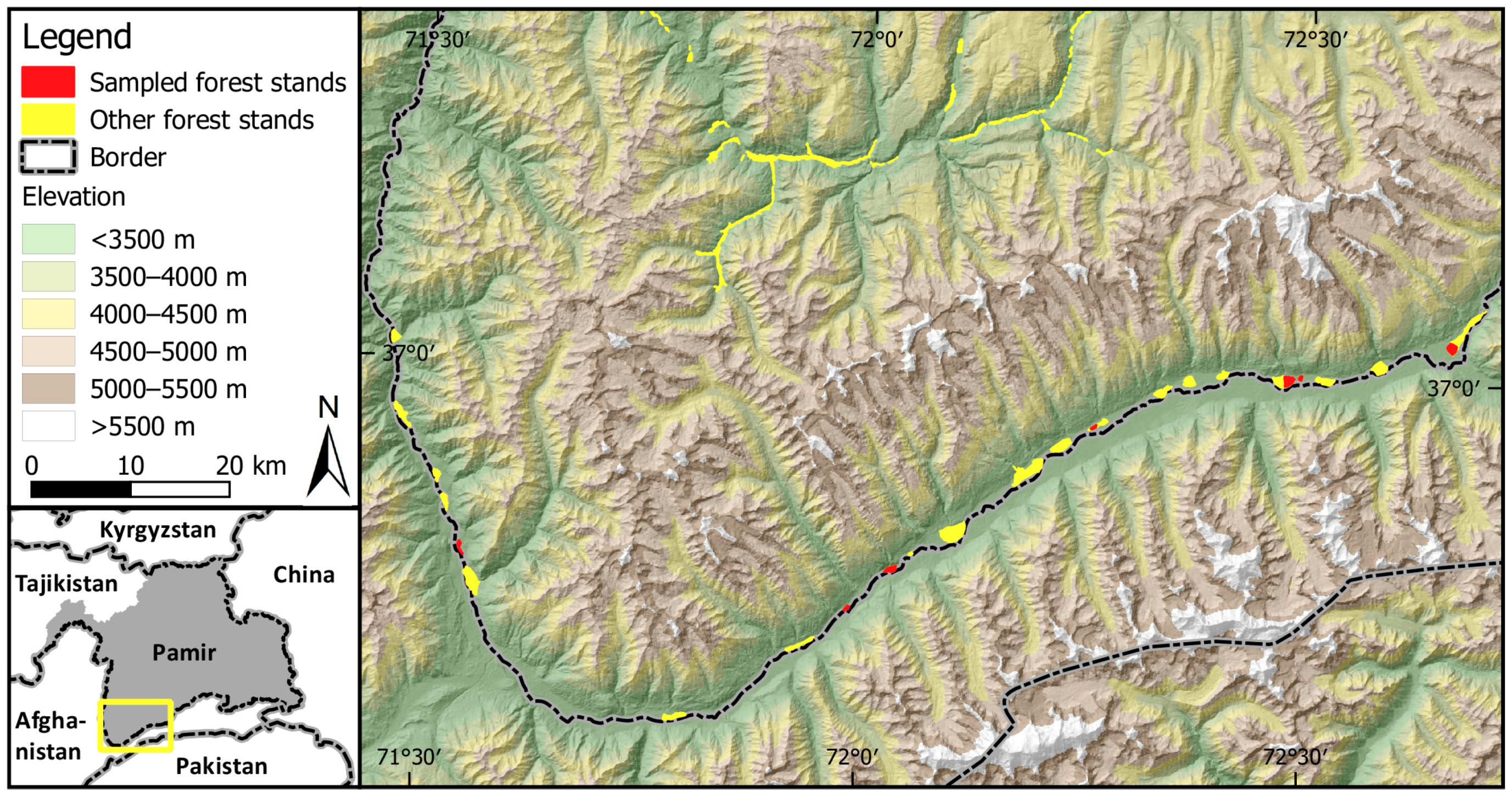
2. Study Area
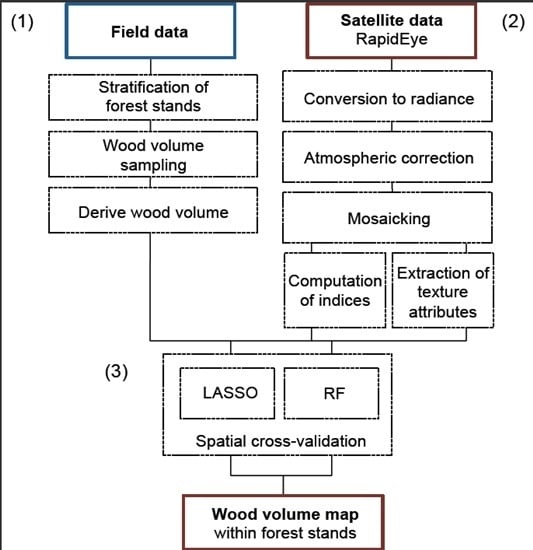
3. Material and Methods
3.1. Field Data
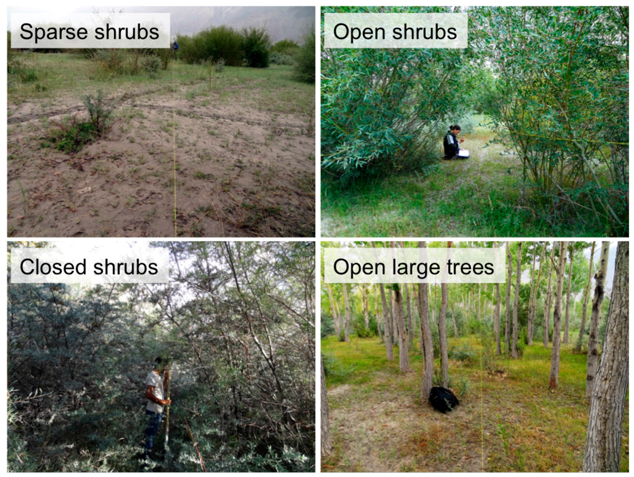
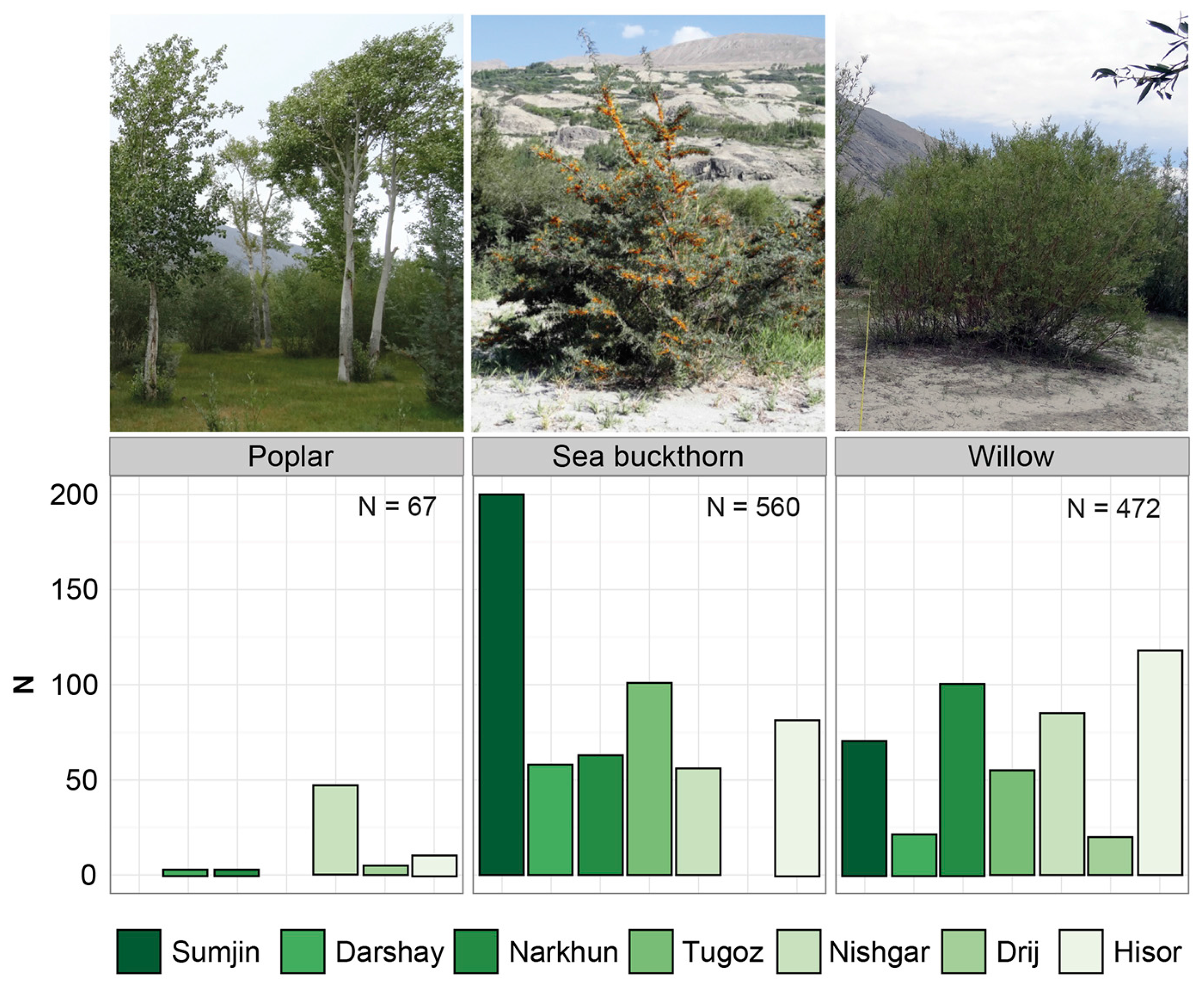
3.1.1. Sampled Woody Species
3.1.2. Field Measurements and Wood Volume Calculation
3.2. Satellite Data
3.3. Modeling Wood Volume
4. Results
4.1. Ground-Based Measured and Calculated Parameters
4.2. Empirical Wood Volume Models and Variable Importance
5. Discussion
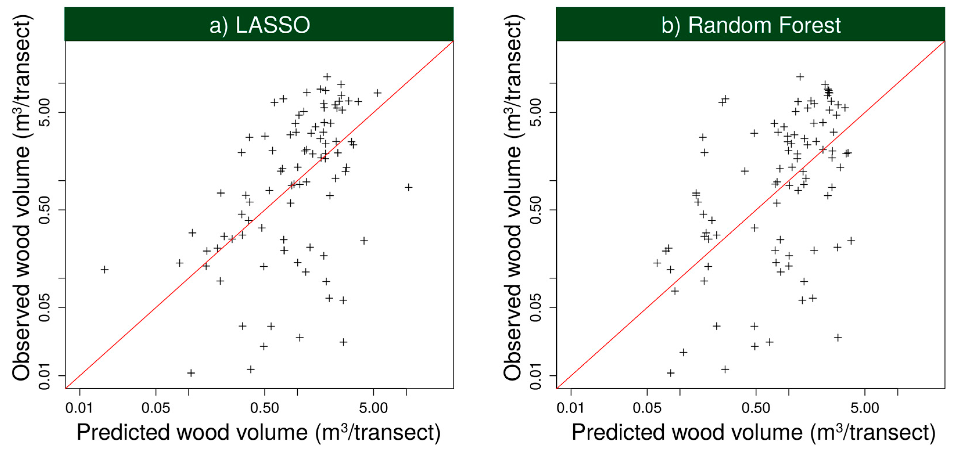
5.1. Model Performance
5.2. Model Uncertainties
5.3. Statistical Performance and Importance of Predictors
6. Conclusions
Acknowledgments
Author Contributions
Conflicts of Interest
References
- Lu, D. The potential and challenge of remote sensing-based biomass estimation. Int. J. Remote Sens. 2006, 27, 1297–1328. [Google Scholar] [CrossRef]
- Millennium Ecosystem Assessment. Ecosystems and Human Well-Being—Synthesis. Available online: http://www.millenniumassessment.org/documents/document.356.aspx.pdf (accessed on 15 February 2015).
- Safriel, U.; Adeel, Z.; Niemeijer, D.; Puigdefabregas, J.; White, R.; Lal, R.; Winslow, M.; Ziedler, J.; Prince, S.; Archer, E.; et al. Dryland systems. In Ecosystems and Human Well-Being: Current State and Trends: Findings of the Condition Trends Work Group; Hassan, R., Scholes, R., Ash, N., Eds.; Island Press: Washington, DC, USA, 2005; Volume 1, pp. 623–662. [Google Scholar]
- Ayanu, Y.Z.; Conrad, C.; Nauss, T.; Wegmann, M.; Koellner, T. Quantifying and mapping ecosystem services supplies and demands: A review of remote sensing applications. Environ. Sci. Technol. 2012, 46, 8529–8541. [Google Scholar] [CrossRef] [PubMed]
- Sarker, L.R.; Nichol, J.E. Improved forest biomass estimates using ALOS AVNIR-2 texture indices. Remote Sens. Environ. 2011, 115, 968–977. [Google Scholar] [CrossRef]
- Eisfelder, C.; Kuenzer, C.; Dech, S. Derivation of biomass information for semi-arid areas using remote-sensing data. Int. J. Remote Sens. 2012, 33, 2937–2984. [Google Scholar] [CrossRef]
- Avitabile, V.; Baccini, A.; Friedl, M.A.; Schmullius, C. Capabilities and limitations of Landsat and land cover data for aboveground woody biomass estimation of Uganda. Remote Sens. Environ. 2012, 117, 366–380. [Google Scholar] [CrossRef]
- Cutler, M.E.J.; Boyd, D.S.; Foody, G.M.; Vetrivel, A. Estimating tropical forest biomass with a combination of SAR image texture and Landsat TM data: An assessment of predictions between regions. ISPRS J. Photogramm. Remote Sens. 2012, 70, 66–77. [Google Scholar] [CrossRef] [Green Version]
- Samimi, C.; Kraus, T. Biomass estimation using Landsat-TM and -ETM+. Towards a regional model for Southern Africa? GeoJ 2004, 59, 177–187. [Google Scholar] [CrossRef]
- Zandler, H.; Brenning, A.; Samimi, C. Quantifying dwarf shrub biomass in an arid environment: Comparing empirical methods in a high dimensional setting. Remote Sens. Environ. 2015, 158, 140–155. [Google Scholar] [CrossRef]
- Asner, G.P.; Wessman, C.A.; Bateson, C.A.; Privette, J.L. Impact of tissue, canopy, and landscape factors on the hyperspectral reflectance variability of arid ecosystems. Remote Sens. Environ. 2000, 74, 69–84. [Google Scholar] [CrossRef]
- Beeri, O.; Phillips, R.; Hendrickson, J.; Frank, A.B.; Kronberg, S. Estimating forage quantity and quality using aerial hyperspectral imagery for northern mixed-grass prairie. Remote Sens. Environ. 2007, 110, 216–225. [Google Scholar] [CrossRef]
- Qi, J.; Wallace, O.; Lansing, E. Biophysical attributes estimation from satellite images in arid regions. In Proceedings of the 2002 IEEE International Geoscience and Remote Sensing Symposium, Toronto, ON, Canada, 24–28 June 2002.
- Svoray, T.; Shoshany, M. Herbaceous biomass retrieval in habitats of complex composition: A model merging sar images with unmixed landsat tm data. IEEE Trans. Geosci. Remote Sens. 2003, 41, 1592–1601. [Google Scholar] [CrossRef]
- Wessels, K.J.; Prince, S.D.; Zambatis, N.; MacFadyen, S.; Frost, P.E.; Van Zyl, D. Relationship between herbaceous biomass and 1-km2 Advanced Very High Resolution Radiometer (AVHRR) NDVI in Kruger National Park, South Africa. Int. J. Remote Sens. 2006, 27, 951–973. [Google Scholar] [CrossRef]
- Brandt, M.; Verger, A.; Diouf, A.A.; Baret, F.; Samimi, C. Local vegetation trends in the sahel of Mali and Senegal using long time series FAPAR satellite products and field measurement (1982–2010). Remote Sens. 2014, 6, 2408–2434. [Google Scholar] [CrossRef]
- Diouf, A.; Lambin, E.F. Monitoring land-cover changes in semi-arid regions: Remote sensing data and field observations in the Ferlo, Senegal. J. Arid Environ. 2001, 48, 129–148. [Google Scholar] [CrossRef]
- Holm, A.M.; Cridland, S.W.; Roderick, M.L. The use of time-integrated NOAA NDVI data and rainfall to assess landscape degradation in the arid shrubland of Western Australia. Remote Sens. Environ. 2003, 85, 145–158. [Google Scholar] [CrossRef]
- Kawamura, K.; Akiyama, T.; Yokota, H.; Tsutsumi, M.; Yasuda, T.; Watanabe, O.; Wang, S. Quantifying grazing intensities using geographic information systems and satellite remote sensing in the Xilingol steppe region, Inner Mongolia, China. Agric. Ecosyst. Environ. 2005, 107, 83–93. [Google Scholar] [CrossRef]
- Tucker, C.J.; Vanpraet, C.L.; Sharman, M.J.; Van Ittersum, G. Satellite remote sensing of total herbaceous biomass production in the senegalese sahel: 1980–1984. Remote Sens. Environ. 1985, 17, 233–249. [Google Scholar] [CrossRef]
- Xu, B.; Yang, X.C.; Tao, W.G.; Miao, J.M.; Yang, Z.; Liu, H.Q.; Jin, Y.X.; Zhu, X.H.; Qin, Z.H.; Lv, H.Y.; et al. MODIS-based remote-sensing monitoring of the spatiotemporal patterns of China’s grassland vegetation growth. Int. J. Remote Sens. 2013, 34, 3867–3878. [Google Scholar] [CrossRef]
- Aranha, J.T.; Viana, H.F.; Rodrigues, R. Vegetation classification and quantification by satellite image processing. A case study in North Portugal. In Proceedings of the 2008 International Conference and Exhibition on Bioenergy: Challenges and Opportunities, Guimarães, Portugal, 6–9 April 2008.
- Kraus, T.; Samimi, C. Biomass estimation for land use management and fire management using Landsat-TM and -ETM+. Erdkunde 2002, 56, 130–143. [Google Scholar] [CrossRef]
- Samimi, C. Das Weidepotential im Gutu Distrikt (Zimbabwe): Möglichkeiten und Grenzen der Modellierung unter Verwendung von Landsat TM-5. Available online: http://www.klimatologie.uni-bayreuth.de/pdf/publications/Das-Weidepotential-im-Gutu-Distrikt.pdf (accessed on 10 November 2015).
- Wylie, B.K.; Meyer, D.J.; Tieszen, L.L.; Mannel, S. Satellite mapping of surface biophysical parameters at the biome scale over the North American grasslands A case study. Remote Sens. Environ. 2002, 79, 266–278. [Google Scholar] [CrossRef]
- Eitel, J.U.H.; Vierling, L.A.; Litvak, M.E.; Long, D.S.; Schulthess, U.; Ager, A.A.; Krofcheck, D.J.; Stoscheck, L. Broadband, red-edge information from satellites improves early stress detection in a New Mexico conifer woodland. Remote Sens. Environ. 2011, 115, 3640–3646. [Google Scholar] [CrossRef]
- Zandler, H.; Brenning, A.; Samimi, C. Potential of space-borne hyperspectral data for biomass quantification in an arid environment: Advantages and limitations. Remote Sens. 2015, 7, 4565–4580. [Google Scholar] [CrossRef]
- Clevers, J.G.P.W.; De Jong, S.M.; Epema, G.F.; Van der Meer, F.D.; Bakker, W.H.; Skidmore, A.K.; Scholte, K.H. Derivation of the red edge index using the MERIS standard. Int. J. Remote Sens. 2002, 23, 3169–3184. [Google Scholar] [CrossRef]
- Brantley, S.T.; Zinnert, J.C.; Young, D.R. Application of hyperspectral vegetation indices to detect variations in high leaf area index temperate shrub thicket canopies. Remote Sens. Environ. 2011, 115, 514–523. [Google Scholar] [CrossRef]
- Vanselow, K.; Samimi, C. Predictive mapping of dwarf shrub vegetation in an arid high mountain ecosystem using remote sensing and random forests. Remote Sens. 2014, 6, 6709–6726. [Google Scholar] [CrossRef]
- Attarchi, S.; Gloaguen, R. Improving the estimation of above ground biomass using dual polarimetric PALSAR and ETM+ data in the Hyrcanian mountain forest (Iran). Remote Sens. 2014, 6, 3693–3715. [Google Scholar] [CrossRef]
- Eckert, S. Improved forest biomass and carbon estimations using texture measures from WorldView-2 satellite data. Remote Sens. 2012, 4, 810–829. [Google Scholar] [CrossRef]
- Kelsey, K.; Neff, J. Estimates of aboveground biomass from texture analysis of Landsat imagery. Remote Sens. 2014, 6, 6407–6422. [Google Scholar] [CrossRef]
- Lu, D. Aboveground biomass estimation using Landsat TM data in the Brazilian Amazon. Int. J. Remote Sens. 2005, 26, 2509–2525. [Google Scholar] [CrossRef]
- Luckman, A.J.; Frery, A.C.; Yanasse, C.C.F.; Groom, G.B. Texture in airborne SAR imagery of tropical forest and its relationship to forest regeneration stage. Int. J. Remote Sens. 1997, 18, 1333–1349. [Google Scholar] [CrossRef]
- Castillo-Santiago, M.Á.; Ghilardi, A.; Oyama, K.; Hernández-Stefanoni, J.L.; Torres, I.; Flamenco-Sandoval, A.; Fernández, A.; Mas, J.-F. Estimating the spatial distribution of woody biomass suitable for charcoal making from remote sensing and geostatistics in central Mexico. Energy Sustain. Dev. 2013, 17, 177–188. [Google Scholar] [CrossRef]
- Forzieri, G. Satellite retrieval of woody biomass for energetic reuse of riparian vegetation. Biomass Bioenergy 2012, 36, 432–438. [Google Scholar] [CrossRef]
- Wiedemann, C.; Salzmann, S.; Mirshakarov, I.; Volkmer, H. Thermal insulation in high mountainous regions. Mt. Res. Dev. 2012, 32, 294–303. [Google Scholar] [CrossRef]
- Mislimshoeva, B.; Hable, R.; Fezakov, M.; Samimi, C.; Abdulnazarov, A.; Koellner, T. Factors influencing households’ firewood consumption in the Western Pamirs, Tajikistan. Mt. Res. Dev. 2014, 34, 147–156. [Google Scholar] [CrossRef]
- Breu, T.; Maselli, D.; Hurni, H. Knowledge for sustainable development in the Tajik Pamir Mountains. Mt. Res. Dev. 2005, 25, 139–146. [Google Scholar] [CrossRef]
- Hoeck, T.; Droux, R.; Breu, T.; Hurni, H.; Maselli, D. Rural energy consumption and land degradation in a post-Soviet setting—An example from the west Pamir mountains in Tajikistan. Energy Sustain. Dev. 2007, 11, 48–57. [Google Scholar] [CrossRef]
- Breckle, S.-W.; Wucherer, W. Vegetation of the Pamir (Tajikistan): Land use and desertification problems. In Land Use Change and Mountain Biodiversity; Spehn, E., Liberman, M., Körner, C., Eds.; CRC Press: Boca Raton, FL, USA, 2006; pp. 225–237. [Google Scholar]
- Schumacher, P. Quantification of Woody Biomass in the Western Pamirs—Assessing Firewood Availability in a Semi-Arid High Mountainous Region Using High Resolution Satellite Data and Field Measurements. Master’s Thesis, University of Bayreuth, Bayreuth, Germany, 2014. [Google Scholar]
- METI, NASA. ASTER Global Digital Elevation Model V002. Sioux Falls, SD. 2009. Available online: https://lpdaac.usgs.gov/dataset_discovery/aster/aster_products_table/astgtm (accessed on 7 August 2015). [Google Scholar]
- Birk, S. Development of the FGIS (Forest Geographical Information System); Interim Mission Report for Deutsche Gesellschaft für Technische Zusammenarbeit (GTZ); Deutsche Gesellschaft für Technische Zusammenarbeit (GTZ) GmbH: Eschborn, Germany, 2009; p. 13. [Google Scholar]
- Mueller-Dombois, D.; Ellenberg, H. Aims and Methods of Vegetation Ecology; John Wiley & Sons: New York, NY, USA, 1974; p. 287. [Google Scholar]
- Coulloudon, B.; Eshelman, K.; Gianola, J.; Habich, N.; Hughes, L.; Johnson, C.; Pellant, M.; Podborny, P.; Rasmussen, A.; Robles, B.; et al. Sampling Vegetation Attributes; BLM Technical Reference 4400-4; Bureau of Land Management's National Applied Resource Sciences Center: Denver, CO, USA, 1999; p. 171. [Google Scholar]
- Akhmadov, K. Forest and Forest Products Country Profile: Tajikistan; Geneva Timber and Forest Discussion Paper 46; United Nations Economic Commission for Europe, Food and Agriculture Organizations of the United Nations: Rome, Italy, 2008; p. 48. [Google Scholar]
- Kirchhoff, J.F.; Fabian, A. Forestry Sector Analysis of the Republic of Tajikistan; Deutsche Gesellschaft für Technische Zusammenarbeit (GTZ): Eschborn, Germany, 2010; p. 56. [Google Scholar]
- Akhmadov, K. Country statement Tajikistan—Forest resources assessment for sustainable forest management. In Proceedings of the Capacity Building in Sharing Forest and Market Information Workshop, Krtiny, Czech Republic, 24–28 October 2005.
- Akhmadov, K.M.; Breckle, S.-W.; Breckle, U. Effects of grazing on biodiversity, productivity, and soil erosion of alpine pastures in Tajik mountains. In Land Use Change and Mountain Biodiversity; Spehn, E., Liberman, M., Körner, C., Eds.; CRC Press: Boca Raton, FL, USA, 2006; pp. 241–250. [Google Scholar]
- Cannell, M.G.R. Woody biomass of forest stands. For. Ecol. Manag. 1984, 8, 299–312. [Google Scholar] [CrossRef]
- Gray, H.R. The Form and Taper of Forest-Tree Stems; Institute Paper No. 32; Imperial Forestry Institute, University of Oxford: Oxford, UK, 1956; p. 84. [Google Scholar]
- Hoyer, G.E. Tree Form Quotients as Variables in Volume Estimation; U.S. Department of Agriculture, Forest Service, Pacific Northwest Forest and Range Experiment Station: Portland, OR, USA, 1985; p. 16. [Google Scholar]
- Van Laar, A.; Akca, A. Forest Mensuration, 1st ed.; Springer: Houten, The Netherlands, 2007; p. 389. [Google Scholar]
- Spiekermann, R.; Brandt, M.; Samimi, C. Woody vegetation and land cover changes in the Sahel of Mali (1967–2011). Int. J. Appl. Earth Observ. Geoinf. 2015, 34, 113–121. [Google Scholar] [CrossRef]
- Zandler, H. Assessment of Woody Biomass and Solar Energy Resources with Remote Sensing and GIS Techniques—A Regional Study in the High Mountains of the Eastern Pamirs (Tajikistan). Ph.D. Thesis, University of Bayreuth, Bayreuth, Germany, September 2015. [Google Scholar]
- Tucker, C.J. Red and photographic infrared linear combinations for monitoring vegetation. Remote Sens. Environ. 1979, 8, 127–150. [Google Scholar] [CrossRef]
- Verrelst, J.; Koetz, B.; Kneubühler, M.; Schaepman, M.; Verrelst, J.; Schaepman, M. Directional Sensitivity Analysis of Vegetation Indices from Multi-Angular CHRIS/PROBA Data. Available online: http://www.isprs.org/proceedings/XXXVI/part7/PDF/227.pdf (accessed on 11 March 2015).
- Gilabert, M.A.; Gonzales-Piqueras, F.J.; Garcıa-Haro, F.; Melia, J. A generalized soil-adjusted vegetation index. Remote Sens. Environ. 2002, 82, 303–310. [Google Scholar] [CrossRef]
- Haralick, R.M.; Shanmugam, K.; Dinstein, I. Textural features for image classification. IEEE Trans. Syst. Man Cybern. 1973, 3, 610–621. [Google Scholar] [CrossRef]
- Dube, T.; Mutanga, O. Investigating the robustness of the new Landsat-8 Operational Land Imager derived texture metrics in estimating plantation forest aboveground biomass in resource constrained areas. ISPRS J. Photogramm. Remote Sens. 2015, 108, 12–32. [Google Scholar] [CrossRef]
- Gitelson, A.; Vina, A.; Ciganda, V.; Rundquist, D.C.; Arkebauer, T.J. Remote estimation of canopy chlorophyll content in crops. Geophys. Res. Lett. 2005, 32, 1–4. [Google Scholar] [CrossRef]
- Gitelson, A.A.; Merzlyak, M.N. Remote estimation of chlorophyll content in higher plant leaves. Int. J. Remote Sens. 1997, 18, 2691–2697. [Google Scholar] [CrossRef]
- Loris, V.; Damiano, G. Mapping the green herbage ratio of grasslands using both aerial and satellite-derived spectral reflectance. Agric. Ecosyst. Environ. 2006, 115, 141–149. [Google Scholar] [CrossRef]
- Wang, F.; Huang, J.; Tang, Y.; Wang, X. New vegetation index and its application in estimating leaf area index of rice. Rice Sci. 2007, 14, 195–203. [Google Scholar] [CrossRef]
- Merzlyak, M.N.; Gitelson, A.A.; Chivkunova, O.B.; Solovchenko, A.E.; Pogosyan, S.I. Application of reflectance spectroscopy for analysis of higher plant pigments. Russ. J. Plant Physiol. 2003, 50, 704–710. [Google Scholar] [CrossRef]
- Barnes, E.; Clarke, T.; Richards, S.; Colaizzi, P.; Haberland, J.; Kostrzewski, P.; Choi, C.; Riley, E.; Thompson, T.; Lascano, R.; et al. Coincident detection of crop water stress, nitrogen status and canopy density using ground-based multispectral data. In Proceedings of the Fifth International Conference on Precision Agriculture, Bloomington, MN, USA, 16–19 July 2000.
- Gitelson, A.; Merzlyak, M.N. Spectral reflectance changes associated with autumn senescence of Aesculus hippocastanum L. and Acer platanoides L. leaves. Spectral features and relation to chlorophyll estimation. J. Plant Physiol. 1994, 143, 286–292. [Google Scholar] [CrossRef]
- Kauth, R.J.; Thomas, G.S. The Tasselled Cap—A Graphic Description of the Spectral-Temporal Development of Agricultural Crops as Seen by Landsat. Available online: http://citeseerx.ist.psu.edu/viewdoc/download?doi=10.1.1.461.6381&rep=rep1&type=pdf (accessed on 14 March 2015).
- Bannari, A.; Morin, D.; Bonn, F.; Huete, A.R. A review of vegetation indices. Remote Sens. Rev. 1995, 13, 95–120. [Google Scholar] [CrossRef]
- Huete, A.R.; Liu, H.Q.; Batchily, K.; Leeuwen, W.V. A comparison of vegetation indices over a global set of TM images for EOS-MODIS. Remote Sens. Rev. 1997, 59, 440–451. [Google Scholar] [CrossRef]
- Huete, A.R. A Soil-Adjusted Vegetation Index (SAVI). Remote Sens. Environ. 1988, 25, 295–309. [Google Scholar] [CrossRef]
- Gitelson, A.A.; Chivkunova, O.B.; Merzlyak, M.N. Nondestructive estimation of anthocyanins and chlorophylls in anthocyanic leaves. Am. J. Bot. 2009, 96, 1861–1868. [Google Scholar] [CrossRef] [PubMed]
- James, G.; Witten, D.; Hastie, T.; Tibshirani, R. An Introduction to Statistical Learning with Applications in R, 1st ed.; Springer: New York, NY, USA, 2013; p. 436. [Google Scholar]
- Hastie, T.; Tibshirani, R.; Friedman, J. The Elements of Statistical Learning: Data Mining, Inference, and Prediction, 2nd ed.; Springer: New York, NY, USA, 2009; p. 750. [Google Scholar]
- Pal, M. Random forest classifier for remote sensing classification. Int. J. Remote Sens. 2005, 26, 217–222. [Google Scholar] [CrossRef]
- Brenning, A. Spatial cross-validation and bootstrap for the assessment of prediction rules in remote sensing: The R package sperrorest. In Proceedings of the 2012 IEEE International Geoscience and Remote Sensing Symposium, Munich, Germany, 22–27 July 2012; pp. 5372–5375.
- Baskerville, G.L. Use of logarithmic regression in the estimation of plant biomass. Can. J. For. Res. 1972, 2, 49–53. [Google Scholar] [CrossRef]
- Strobl, C.; Boulesteix, A.-L.; Zeileis, A.; Hothorn, T. Bias in random forest variable importance measures: Illustrations, sources and a solution. BMC Bioinform. 2007, 8. [Google Scholar] [CrossRef] [PubMed] [Green Version]
- Brenning, A. Spatial Error Estimation and Variable Importance: R Package “Sperrorest”. Available online: https://cran.r-project.org/web/packages/ (accessed on 16 June 2015).
- Friedman, A.J.; Hastie, T.; Simon, N.; Tibshirani, R. Lasso and Elastic-Net Regularized Generalized Linear Models: R Package “Glmnet”. Available online: https://cran.r-project.org/web/packages/ (accessed on 16 June 2015).
- Liaw, A.; Wiener, M. Breiman and Cutler’s Random Forests for Classification and Regression: R Package “Randomforest”. Available online: https://cran.r-project.org/web/packages/ (accessed on 16 June 2015).
- Brenning; Alexander SAGA Geoprocessing and Terrain Analysis in R: R Package “RSAGA”. Available online: https://cran.r-project.org/web/packages/ (accessed on 16 June 2015).
- Ali, M.; Montzka, C.; Stadler, A.; Menz, G.; Thonfeld, F.; Vereecken, H. Estimation and validation of RapidEye-based time-series of leaf area index for winter wheat in the Rur Catchment (Germany). Remote Sens. 2015, 7, 2808–2831. [Google Scholar] [CrossRef]
- Kross, A.; McNairn, H.; Lapen, D.; Sunohara, M.; Champagne, C. Assessment of RapidEye vegetation indices for estimation of leaf area index and biomass in corn and soybean crops. Int. J. Appl. Earth Observ. Geoinf. 2015, 34, 235–248. [Google Scholar] [CrossRef]
- Li, X.; Gao, Z.; Bai, L.; Huang, Y. Potential of high resolution RapidEye data for sparse vegetation fraction mapping in arid regions. In Proceedings of the 2012 IEEE International Geoscience and Remote Sensing Symposium, Munich, Germany, 22–27 July 2012; pp. 420–423.
- Ramoelo, A.; Skidmore, A.K.; Cho, M.A.; Schlerf, M.; Mathieu, R.; Heitkönig, I.M.A. Regional estimation of savanna grass nitrogen using the red-edge band of the spaceborne RapidEye sensor. Int. J. Appl. Earth Observ. Geoinf. 2012, 19, 151–162. [Google Scholar] [CrossRef]
- Ren, H.; Zhou, G.; Zhang, X. Estimation of green aboveground biomass of desert steppe in Inner Mongolia based on red-edge reflectance curve area method. Biosyst. Eng. 2011, 109, 385–395. [Google Scholar] [CrossRef]
- Cho, M.A.; Skidmore, A.K. Hyperspectral predictors for monitoring biomass production in Mediterranean mountain grasslands: Majella National Park, Italy. Int. J. Remote Sens. 2009, 30, 499–515. [Google Scholar] [CrossRef]
- Fuchs, H.; Magdon, P.; Kleinn, C.; Flessa, H. Estimating aboveground carbon in a catchment of the Siberian forest tundra: Combining satellite imagery and field inventory. Remote Sens. Environ. 2009, 113, 518–531. [Google Scholar] [CrossRef]
- Powell, S.L.; Cohen, W.B.; Healey, S.P.; Kennedy, R.E.; Moisen, G.G.; Pierce, K.B.; Ohmann, J.L. Quantification of live aboveground forest biomass dynamics with Landsat time-series and field inventory data: A comparison of empirical modeling approaches. Remote Sens. Environ. 2010, 114, 1053–1068. [Google Scholar] [CrossRef]
- Shoshany, M.; Svoray, T. Multidate adaptive unmixing and its application to analysis of ecosystem transitions along a climatic gradient. Remote Sens. Environ. 2002, 82, 5–20. [Google Scholar] [CrossRef]
- Immitzer, M.; Vuolo, F.; Atzberger, C. First experience with Sentinel-2 data for crop and tree species classifications in central Europe. Remote Sens. 2016, 8. [Google Scholar] [CrossRef]
- Radoux, J.; Chomé, G.; Jacques, D.C.; Waldner, F.; Bellemans, N.; Matton, N.; Lamarche, C.; d’Andrimont, R.; Defourny, P. Sentinel-2’s potential for sub-pixel landscape feature detection. Remote Sens. 2016, 8. [Google Scholar] [CrossRef]
- Lazaridis, D.C.; Verbesselt, J.; Robinson, A.P. Penalized regression techniques for prediction: A case study for predicting tree mortality using remotely sensed vegetation indices. Can. J. For. Res. 2011, 41, 24–34. [Google Scholar] [CrossRef]


| Indices | Description/Equations | References |
|---|---|---|
| Single Bands | Represent reflectance values within respective spectral range | |
| B1–B5 | ||
| Band Ratios | Detect spectral differences and, thus, differences in surface properties | |
| B1/B2–B1/B5; B2/B3–B2/B5; B3/B4–B3/B5; B4/B5 | ||
| Broadband Greenness VIs | Try to measure and display the overall amount of photosynthetic material in vegetation | Tucker [58] |
| Chlorophyll Index Green/Chlorophyll Green Model | Gitelson et al. [63] | |
| Green Normalized Difference Vegetation Index | Gitelson and Merzylak [64], Loris and Damiano [65] | |
| Green Blue Normalized Difference Vegetation Index | Wang et al. [66] | |
| Normalized Difference Vegetation Index | Tucker [58] | |
| Red edge indices | Use reflectance measurements in red edge reflectance portion | Verrelst et al. [59] |
| Browning Reflectance Index | Merzylak et al. [67] | |
| Canopy Chlorophyll Content Index | Barnes et al. [68] | |
| Normalized DifferenceNear-Infrared Red Edge | Barnes et al. [68], Gitelson and Merzylak [69] | |
| Normalized DifferenceRed Edge Red | ||
| Tasseled Cap: Soil Brightness Index | TCSBI = 0.332 × G + 0.603 × R + 0.675 × RE − 0.262 × NIR | Kauth and Thomas [70], Bannari et al. [71] |
| Soil Adjusted VIs | Attempt to minimize the effect of soil background as one source of variation by integrating soil adjustment parameters | Gilabert et al. [60] |
| Enhanced Vegetation Index | Huete et al. [72] | |
| Soil Adjusted Vegetation Index | Huete [73] | |
| Leaf Pigments | Measures stress-related pigments present in vegetation | Verrelst et al. [59] |
| Anthocyanin Reflectance Index | Gitelson et al. [74] | |
| Texture Information | Detect structural details of surface | Haralick et al. [61] |
| Single Bands | TB1–TB5 | |
| Band Ratios | TB1/TB2–TB1/TB5; TB2/TB3–TB2/TB5; TB3/TB4–TB3/TB5; TB4/TB5 |
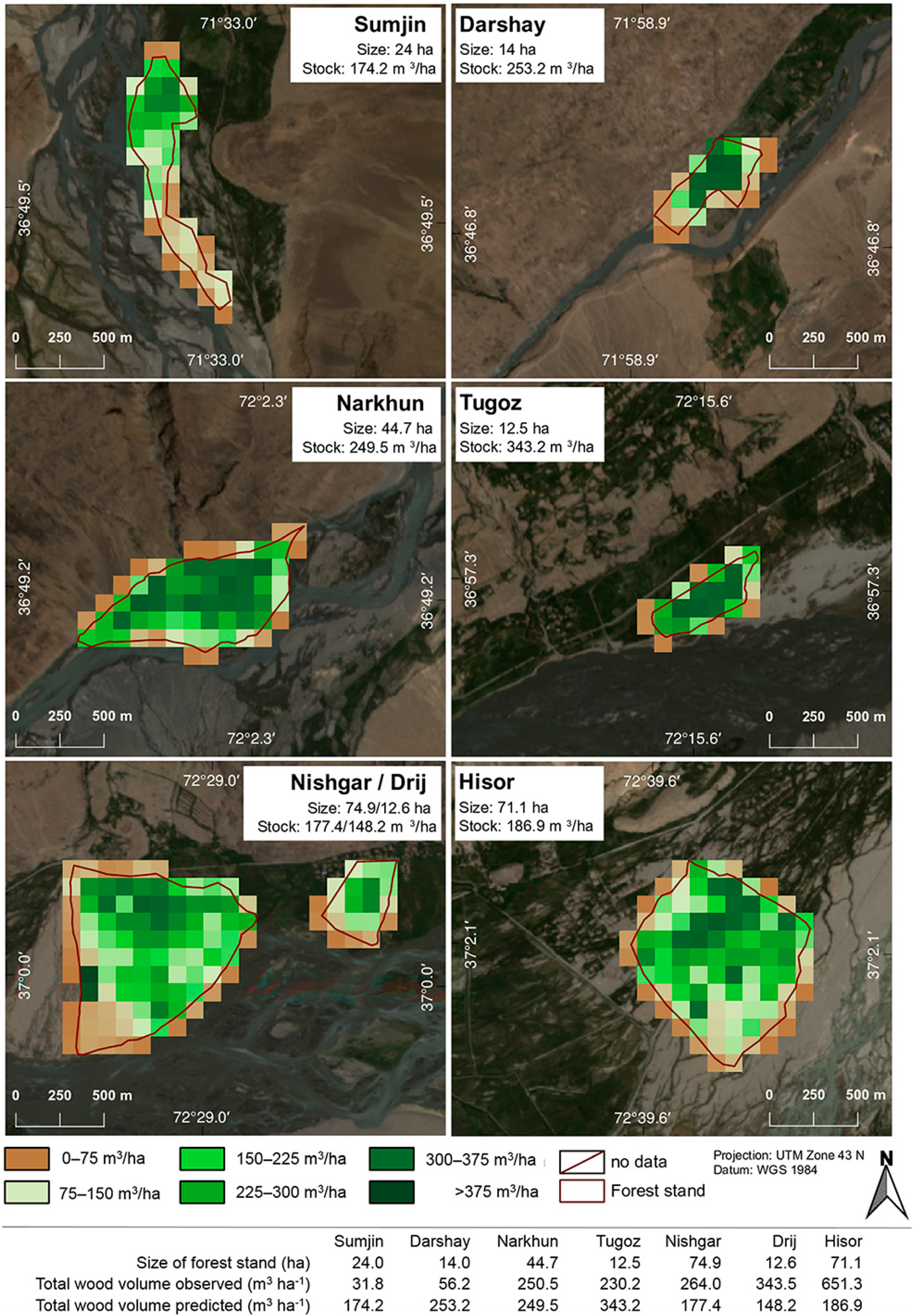
| Sumjin | Darshay | Narkhun | Tugoz | Nishgar | Drij | Hisor | |
|---|---|---|---|---|---|---|---|
| Size of forest stand (ha) | 24 | 14 | 44.7 | 12.5 | 74.9 | 12.6 | 71.1 |
| Total wood volume (m3·ha−1) observed in the field | 31.8 | 56.2 | 250.5 | 230.2 | 264.0 | 343.5 | 651.3 |
| Total wood volume (m3·ha−1) estimated by remote sensing | 174.2 | 253.2 | 249.5 | 343.2 | 177.4 | 148.2 | 186.9 |
| Poplar (N = 67) | |||||||
| No. of trees (per ha) | - | 39 | 28 | - | 336 | 179 | 110 |
| Height (m) | - | 6.6 | 6.5 | - | 6.8 | 7.0 | 10.5 |
| Diameter at breast height (1.3 m) (cm) | - | 9.5 | 14.2 | - | 15.9 | 35.0 | 28.7 |
| Wood volume (m3·ha−1) | - | 2.3 | 3.7 | - | 68.1 | 101.6 | 84.5 |
| Sea buckthorn (N = 560) | |||||||
| No. of trees (per ha) | 2352 | 1442 | 625 | 1923 | 276 | - | 480 |
| Height (m) | 1.9 | 2.4 | 1.8 | 1.9 | 1.5 | - | 1.9 |
| Diameter at knee height (0.3 m) (cm) | 5.0 | 4.8 | 5.0 | 6.5 | 2.5 | - | 5.3 |
| Wood volume (m3·ha−1) | 31.1 | 10.6 | 6.0 | 43.5 | 21.3 | - | 18.6 |
| Willow (N = 472) | |||||||
| No. of trees (per ha) | 636 | 404 | 1250 | 1077 | 827 | 714 | 1260 |
| Height (m) | 2.1 | 2.4 | 2.8 | 5.2 | 2.1 | 2.7 | 3.0 |
| Diameter at knee height (0.3 m) (cm) | 10.0 | 13.7 | 32.8 | 23.7 | 25.5 | 42.9 | 40.5 |
| Wood volume (m3·ha−1) | 6.2 | 11.7 | 180.3 | 172.4 | 58.3 | 182.8 | 282.8 |
| Predictor Set 1 1 | Predictor Set 2 2 | Predictor Set 3 3 | Predictor Set 3 | |
|---|---|---|---|---|
| Broadband VIs | Broadband VIs + Red Edge | Broadband VIs + Red Edge + Texture | Broadband VIs + Red Edge + Texture (log10 wood volume) | |
| LASSO | ||||
| Bias (m3·ha−1) | 265 | 267.5 | 222.5 | 222.5 |
| Standard Deviation (m3·ha−1) | 697.5 | 687.5 | 655 | 348.3 |
| RMSE (m3·ha−1) | 745 | 735 | 687.5 | 687.5 |
| RMSErel (%) | 130 | 128 | 118 | 120 |
| Correlation between observed and predicted | 0.01 (R2) | 0.01 (R2) | 0.10 (R2) | 0.27 (R2) |
| 0.12 (PC 4) | 0.13 (PC) | 0.31 (PC) | 0.52 (PC) | |
| 0.33 (SC 5) | 0.26 (SC) | 0.51 (SC) | 0.51 (SC) | |
| Random Forest | ||||
| Bias (m3·ha−1) | 220 | 207.5 | 265 | 265 |
| Standard Deviation (m3·ha−1) | 687.5 | 672.5 | 617.5 | 241.8 |
| RMSE (m3·ha−1) | 717.5 | 700 | 667.5 | 667.5 |
| RMSErel (%) | 125 | 122 | 117 | 117 |
| Correlation between observed and predicted | 0.04 (R2) | 0.06 (R2) | 0.16 (R2) | 0.26 (R2) |
| 0.20 (PC) | 0.25 (PC) | 0.40 (PC) | 0.51 (PC) | |
| 0.33 (SC) | 0.37 (SC) | 0.50 (SC) | 0.50 (SC) |
© 2016 by the authors; licensee MDPI, Basel, Switzerland. This article is an open access article distributed under the terms and conditions of the Creative Commons Attribution (CC-BY) license (http://creativecommons.org/licenses/by/4.0/).
Share and Cite
Schumacher, P.; Mislimshoeva, B.; Brenning, A.; Zandler, H.; Brandt, M.; Samimi, C.; Koellner, T. Do Red Edge and Texture Attributes from High-Resolution Satellite Data Improve Wood Volume Estimation in a Semi-Arid Mountainous Region? Remote Sens. 2016, 8, 540. https://0-doi-org.brum.beds.ac.uk/10.3390/rs8070540
Schumacher P, Mislimshoeva B, Brenning A, Zandler H, Brandt M, Samimi C, Koellner T. Do Red Edge and Texture Attributes from High-Resolution Satellite Data Improve Wood Volume Estimation in a Semi-Arid Mountainous Region? Remote Sensing. 2016; 8(7):540. https://0-doi-org.brum.beds.ac.uk/10.3390/rs8070540
Chicago/Turabian StyleSchumacher, Paul, Bunafsha Mislimshoeva, Alexander Brenning, Harald Zandler, Martin Brandt, Cyrus Samimi, and Thomas Koellner. 2016. "Do Red Edge and Texture Attributes from High-Resolution Satellite Data Improve Wood Volume Estimation in a Semi-Arid Mountainous Region?" Remote Sensing 8, no. 7: 540. https://0-doi-org.brum.beds.ac.uk/10.3390/rs8070540