Evaluation of Generative Modeling Techniques for Frequency Responses †


IDLab, Department of Information Technology, Ghent University-imec, Technologiepark-Zwijnaarde 126, 9000 Ghent, Belgium
*
Author to whom correspondence should be addressed.
†
Presented at the 1st International Electronic Conference—Futuristic Applications on Electronics, 1–30 November 2020; Available online: https://iec2020.sciforum.net/ .
Eng. Proc. 2020, 3(1), 7; https://0-doi-org.brum.beds.ac.uk/10.3390/IEC2020-06970
Published: 30 October 2020
(This article belongs to the Proceedings of 1st International Electronic Conference—Futuristic Applications on Electronics)
Abstract
:During microwave design, it is of practical interest to obtain insight in the statistical variability of a device’s frequency response with respect to several sources of variation. Unfortunately, the frequency response acquisition can be particularly time-consuming or expensive. This makes uncertainty quantification unfeasible when dealing with complex networks. Generative modeling techniques that are based on machine learning can reduce the computation load by learning the underlying stochastic process from few instances of the device response and generating new ones by executing an inexpensive sampling strategy. This way, an arbitrary number of frequency responses can be obtained that are drawn from a probability distribution that resembles the original one. The use of Gaussian Process Latent Variable Models (GP-LVM) and Variational Autoencoders (VAE) as modeling algorithms will be evaluated in a generative framework. The framework includes a Vector Fitting (VF) pre-processing step which guarantees stability and reciprocity of S-matrices by converting them into a suitable rational model. Both GP-LVM and VAE are tested on the S-parameter responses of two linear multi-port network examples.
1. Introduction
In recent years, efficient and accurate uncertainty quantification methods have become a critical resource for the design on modern RF and microwave circuits. Indeed, due to the increasing integration and miniaturization capabilities, the performance of such circuits is largely affected by the tolerances of the manufacturing process. Typically, performing uncertainty quantification requires to obtain a large number of statistical samples (or instances), which is time-consuming and costly. Hence, several stochastic modeling techniques have been presented in recent years to overcome these limitations, for example based on the Polynomial Chaos (PC) expansion [1] or on Stochastic Reduced Order Models (SROM) [2].
Recently, novel techniques have been presented in the literature based on generative modeling [3,4]. The main advantage of such methods is that uncertainty quantification can be performed with accuracy and efficiency, independently on how many geometrical or electrical parameters of the system under study are under stochastic effects. Generative models are able to efficiently generate a large set of frequency responses whose distribution closely matches that of the system under study, starting from a limited set of training data. Such training data is a small set of frequency responses, which can be obtained via simulations or measurements.
In the following paper, we analyze a generative approach which can employ GP-LVM or VAE as generative model. Different to the technique [4] that directly models the sampled frequency response via the VAE, we investigate a two-step approach, as proposed in [3]. Firstly, a suitable rational model of the training data is obtained via the Vector Fitting algorithm (VF) [5]. Then, the generative model is trained to describe and reproduce the stochastic variations of the rational model’s parameters. Note that the stability and reciprocity of the system under study are guaranteed due to the VF characterization, while passivity is enforced by rejection. We analyze both GP-LVM’s and VAE’s capability to reproduce the data yielded by the rational representation, as well as complex relations between the frequency response and the design parameters.
2. Methodology
Our technique follows the workflow in Figure 1. The first step is converting few initial scattering parameter (S-parameter) instances, which constitute the training set, into rational form coefficients. This is executed by means of the VF algorithm, as described in Section 2.1. Then, the generative modeling algorithm is trained to reproduce the probability distribution of the rational coefficients, given a latent space prior distribution. Next, new S-parameter instances can be obtained by drawing samples from the model’s latent space and extracting the corresponding output of the rational model. New instances are drawn until reaching a suitable number of passive responses. In order to evaluate the accuracy of the proposed method, Section 2.4 presents a suitable similarity metric, which is employed to compare the distribution of a large set of instances drawn from the computed generative model and from the system under study (also called validation set).
2.1. Vector Fitting
Starting from a set of S-matrix frequency samples, the VF algorithm [5] computes a rational model in a pole/residue form as
where s is the complex frequency variable, while and are poles and residues, respectively. The set of poles and residues fully determines the frequency behaviour of each S-matrix element. Since the location of the poles fluctuates amongst different frequency responses realizations, it is decided to model them using a common pole set . Thereby, one instance is only represented by by a set of residues for each S-matrix element. Once a new set of residues are produced by the generative model, S-parameters can be extracted from the corresponding rational form by evaluating it on the desired frequency points.
2.2. Gaussian Process Latent Variable Model
In this framework, the purpose of the generative model is to reproduce the distribution of observed residues data Y, given a distribution of variables X in a latent space of lower dimensionality. Thus, the objective is to extract marginal probability from the joint probability of Y and X:
where is the likelihood function, while is the prior of the latent variables. Assuming that the underlying stochastic process of the S-parameters is Gaussian, a standard normal density can be assigned to the prior . The GP-LVM [6] performs a mapping from the latent space to the observed space using Gaussian Processes (GPs); each dimension d of the data vectors in Y is modeled by an independent GP, such that the likelihood function becomes:
where represents the observations vector of the residue in Y, whereas is a specified kernel function matrix. For this application, the Automatic Relevance Detection (ARD) kernel is chosen, while the variational lower bound [6] is maximized to obtain the marginalized likelihood and optimize GPs hyperparameters accordingly. The GP-LVM allows to predict a new instance of residue data, by evaluating the GPs on a sample drawn from the latent space prior.
2.3. Variational Autoencoder
The Variational Autoencoder [7] provides a different method of modeling the marginal probability , while assuming the same prior for the latent space variables: . Unlike the GP-LVM, the VAE maps the latent space to the observed space by learning simultaneously the posterior distribution and the likelihood. This technique leverages on Bayesian inference to approximate with a parameterized variational distribution , where is a suitable parameter of the model. This allows one to compute the posterior distribution by minimizing a dissimilarity metric between p and q. For this purpose, the distance is usually defined as the Kullback-Leibler divergence :
At the same time, the conditional likelihood can be parameterized over a suitable model parameter, indicated with , and optimized by maximizing its marginal log-likelihood . These two tasks can be combined into a single maximization of a variational lower bound :
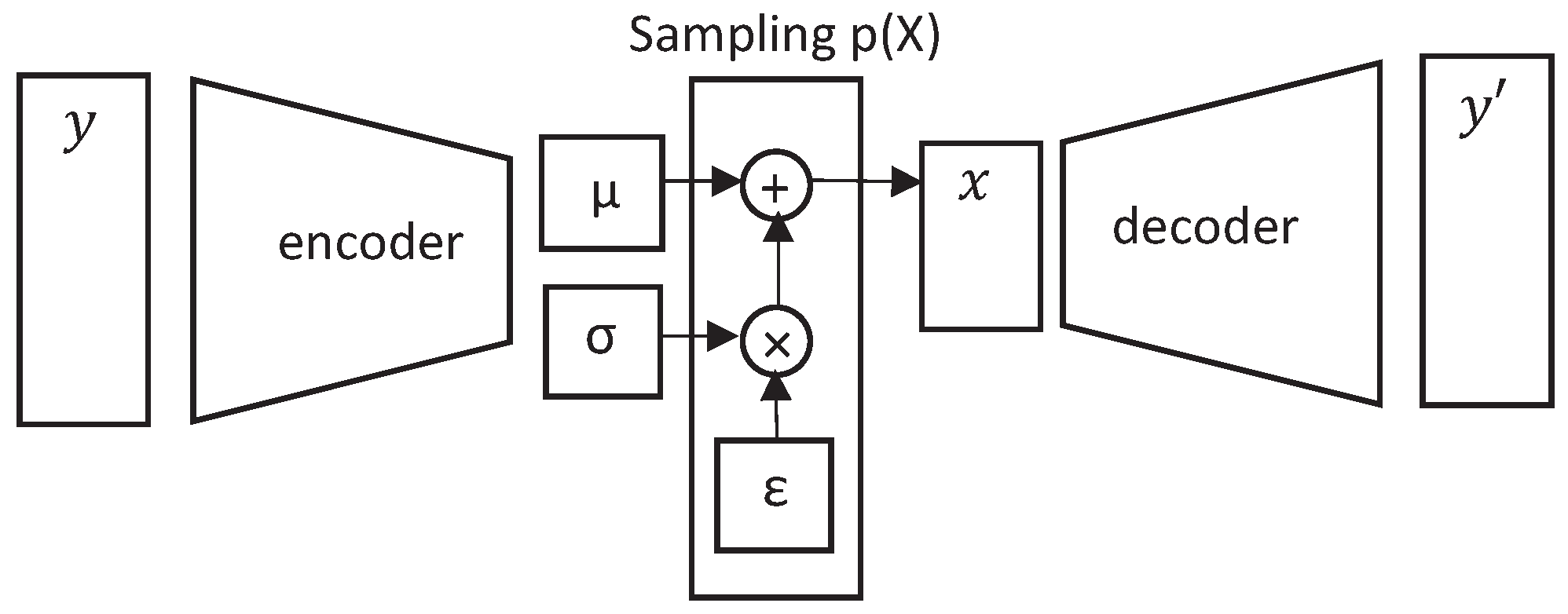
where are the model parameters. The latent space mapping is modeled by a neural network in an encoder-decoder architecture (Figure 2). The encoder represents an input instance y as a sample of , defined by the mean () and the standard deviation (), while the decoder converts a sample from the posterior into an instance of the observable space, reconstructing the initial input . Adding an intermediate sampling operation allows one to produce by drawing a sample from a standard Gaussian distribution:
where d is every latent space dimension. This strategy, known as “reparametrization trick”, enables backpropagation, so that the network can be trained by maximizing the variational lower bound [7]. Indeed, the training forces the encoder to approximate , reducing the KL divergence. In this manner, the network can generate a new instance by directly drawing a sample from the Gaussian prior and evaluating the corresponding decoder output.
2.4. Similarity Metric
The similarity between the distribution of the generated samples and the original one is estimated by the Cramer-Von-Mises (CM) statistic [8]. The CM distance can be computed on two sets of S-parameters, drawn respectively from the generated samples and the validation set, which are relative to the same frequency value. Thus, lower CM scores indicate higher similarity between the distributions. Note that, in our problem setting, the CM score is computed for each frequency sample of the computed S-parameters.
3. Results and Discussion
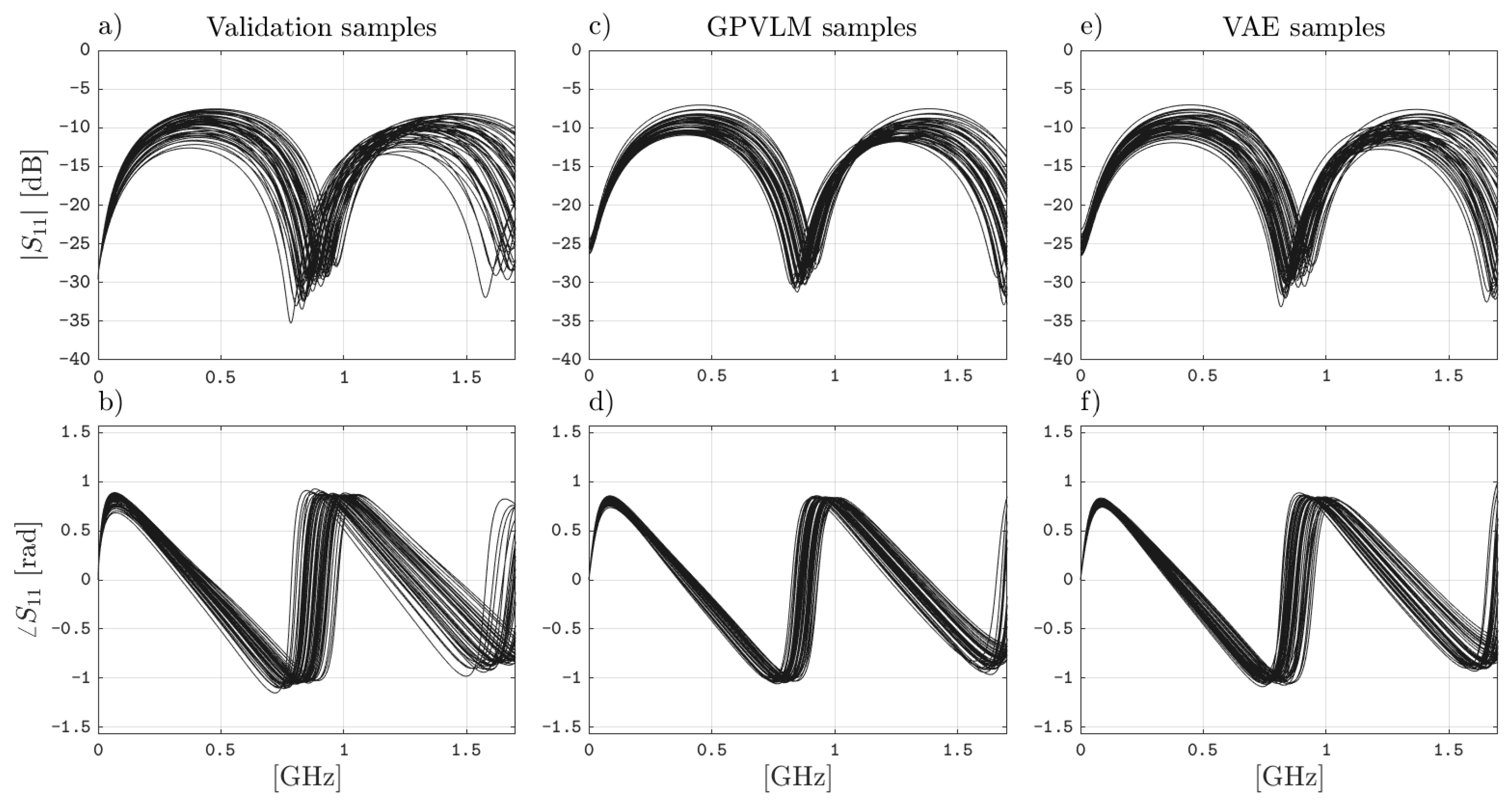
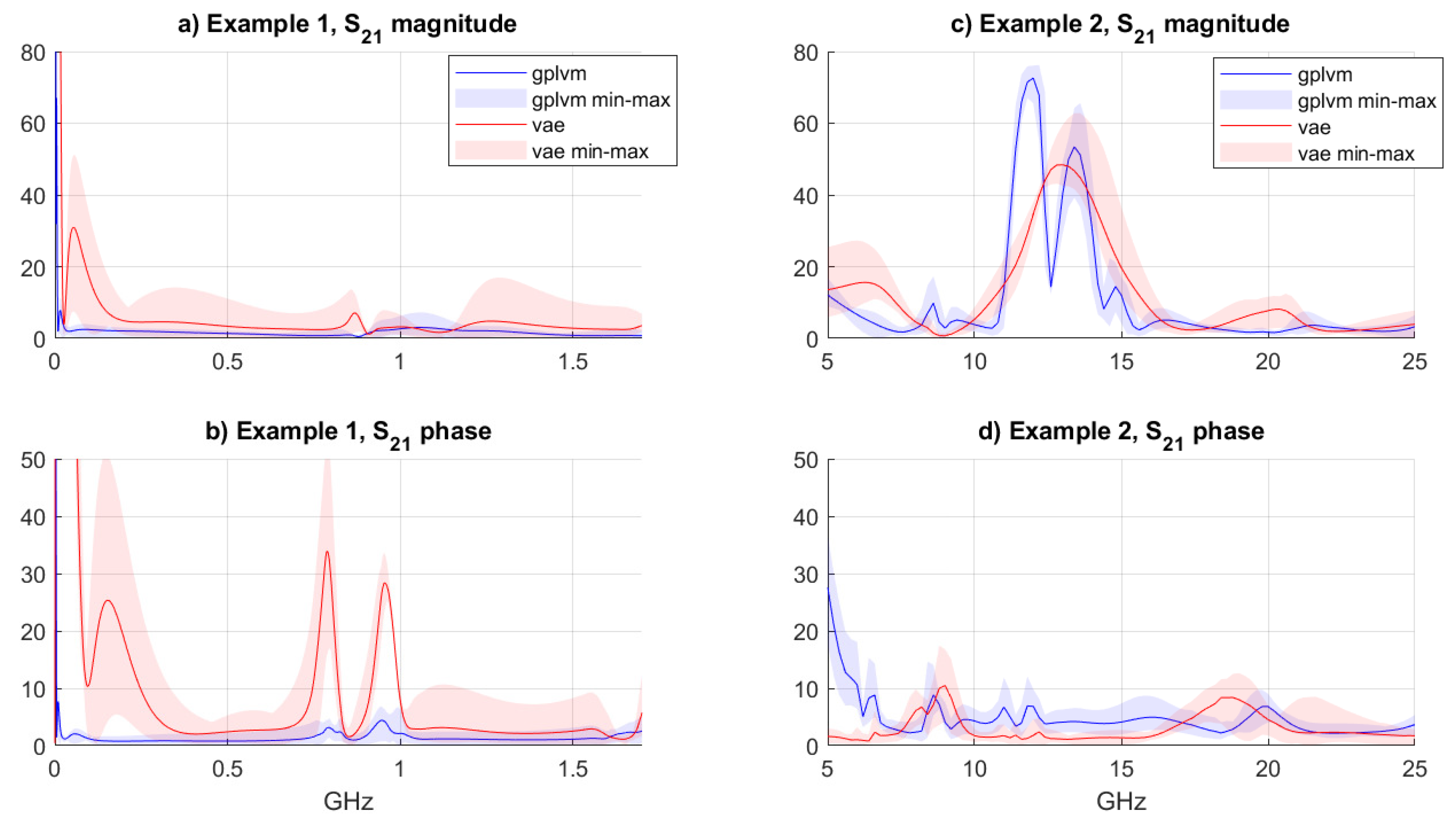
The proposed modeling framework is tested on a two microstrip devices—a pair of coupled transmission lines [3] and a folded-stub notch filter [9]. Their responses are computed using the settings in Table 1, via the simulator ADS Momentum [10]. Training and validation sets are obtained by varying several design parameters, whose value is chosen by sampling independent Gaussian distributions—each distribution has the same standard deviation and is centered in its parameter nominal value. The VF algorithm, as described in Section 2.1, converts the training instances into the corresponding rational form, which is then fed to the generative model. The order of the rational model, which corresponds to the number of poles and residues, is reported in Table 1. After training the GP-LVM and the VAE, as indicated in Section 2.2 and Section 2.3, new S-matrices instances are generated until 1000 passive frequency responses are reached. The complete workflow is repeated 10 times on different training sets for a more accurate validation. Figure 3 illustrates results for the parameter: 50 samples are drawn from the validation set, and the learnt distributions of the GP-LVM and VAE, respectively. The generated samples closely match the original ones, demonstrating a comparable accuracy of the generative models. Finally, the Figure 4 reports the CM score for the generated parameter. In Example 1, the GP-LVM shows a lower score, that is, better accuracy, across all the frequency bandwidth. On the other hand, the VAE appears more accurate in Example 2. It is worth noting that the folded-stub filter presents a wide-band and highly variable frequency response: this causes higher CM-scores for both generative models in Example 2. Thus, both GP-LVM and VAE can be valuable when the framework is applied on new microwave devices.
4. Conclusions
This paper analyses a VF-based generative modeling framework, which is used to produce a large number of S-parameter responses starting from a small set of available samples. Two generative models, the GP-LVM and the VAE, are tested in the framework, estimating their accuracy on two application examples. Both models show adequate performance and constitute a valuable tool to reduce the computation load of frequency responses acquisition.
Funding
This work has been supported by the Flemish Government under the “Onderzoeksprogramma Artificiële Intelligentie (AI) Vlaanderen” and the “Fonds Wetenschappelijk Onderzoek (FWO)” programs.
References
- Ye, Y.; Spina, D.; Manfredi, P.; Ginste, D.V.; Dhaene, T. A Comprehensive and Modular Stochastic Modeling Framework for the Variability-Aware Assessment of Signal Integrity in High-Speed Links. IEEE Trans. Electromagn. Compat. 2018, 60, 459–467. [Google Scholar] [CrossRef]
- Fei, Z.; Huang, Y.; Zhou, J.; Xu, Q. Uncertainty Quantification of Crosstalk Using Stochastic Reduced Order Models. IEEE Trans. Electromagn. Compat. 2017, 59, 228–239. [Google Scholar] [CrossRef]
- De Ridder, S.; Deschrijver, D.; Manfredi, P.; Dhaene, T.; Vande Ginste, D. Generation of Stochastic Interconnect Responses via Gaussian Process Latent Variable Models. IEEE Trans. Electromagn. Compat. 2018, 61, 582–585. [Google Scholar] [CrossRef]
- Ma, X.; Raginsky, M.; Cangellaris, A.C. A Machine Learning Methodology for Inferring Network S-parameters in the Presence of Variability. In Proceedings of the 2018 IEEE 22nd Workshop on Signal and Power Integrity (SPI), Brest, France, 22–25 May 2018. [Google Scholar]
- Gustavsen, B.; Semlyen, A. Rational approximation of frequency domain responses by vector fitting. IEEE Trans. Power Deliv. 1999, 14, 1052–1061. [Google Scholar] [CrossRef]
- Titsias, M.; Lawrence, N.D. Bayesian Gaussian process latent variable model. In Proceedings of the Thirteenth International Conference on Artificial Intelligence and Statistics, Sardinia, Italy, 13–15 May 2010; pp. 844–851. [Google Scholar]
- Kingma, D.P.; Welling, M. Auto-Encoding Variational Bayes. arXiv 2013, arXiv:1312.6114v10. [Google Scholar]
- Anderson, T.W. On the distribution of the two-sample Cramer-von Mises criterion. Ann. Math. Stat. 1962, 33, 1148–1159. [Google Scholar] [CrossRef]
- De Ridder, S.; Deschrijver, D.; Spina, D.; Vande Ginste, D.; Dhaene, T. Statistical modeling of frequency responses using linear Bayesian vector fitting. Int. J. Numer. Model. Electron. Netw. Devices Fields 2020. [Google Scholar] [CrossRef]
- Keysight EEsof EDA, Advanced Design System, 471. Update 1.0. 2018. Avaliable online: https://www.keysight.com/cn/zh/assets/7018-01027/brochures/5988-3326.pdf (accessed on 14 October 2020).
Figure 1.
Workflow of the proposed methodology.

Figure 2.
VAE neural network architecture.

Figure 3.
Magnitude and phase of 50 samples drawn from validation set of Example 1 (a,b), samples generated by the Gaussian Process-Latent Variable Model, (c,d), samples generated by the VAE (e,f).
Figure 3.
Magnitude and phase of 50 samples drawn from validation set of Example 1 (a,b), samples generated by the Gaussian Process-Latent Variable Model, (c,d), samples generated by the VAE (e,f).

Figure 4.
Cramer-Von-Mises (CM)-score of the generated distribution of parameter, for both application examples. The solid line represents the average score across 10 runs on different training sets, while the shaded area covers the range between the minimum and the maximum score recorded.
Figure 4.
Cramer-Von-Mises (CM)-score of the generated distribution of parameter, for both application examples. The solid line represents the average score across 10 runs on different training sets, while the shaded area covers the range between the minimum and the maximum score recorded.


Table 1.
Examples simulation settings.
| Example 1: Pair of Couple Transmission Lines | Example 2: Folded-Stub Notch Filter | |
|---|---|---|
| Frequency range [GHz] | 0–1.8 | 5–25 |
| Frequency step [GHz] | 0.0017 | 0.2 |
| Selected ports | [1, 2] | [1,2] |
| Design parameters | substrate height and permittivity, line widths, line spacing | substrate height and permittivity, stubs spacing, stubs length |
| No. of design parameters | 5 | 4 |
| Parameters standard deviation | 10% of nom.value | 5% of nom.value |
| No. training instances | 50 | 100 |
| No. validation instances | 950 | 300 |
| Rational model order | 10 | 20 |
Publisher’s Note: MDPI stays neutral with regard to jurisdictional claims in published maps and institutional affiliations. |
© 2020 by the authors. Licensee MDPI, Basel, Switzerland. This article is an open access article distributed under the terms and conditions of the Creative Commons Attribution (CC BY) license (https://creativecommons.org/licenses/by/4.0/).
Share and Cite
MDPI and ACS Style
Garbuglia, F.; Spina, D.; Deschrijver, D.; Dhaene, T. Evaluation of Generative Modeling Techniques for Frequency Responses. Eng. Proc. 2020, 3, 7. https://0-doi-org.brum.beds.ac.uk/10.3390/IEC2020-06970
AMA Style
Garbuglia F, Spina D, Deschrijver D, Dhaene T. Evaluation of Generative Modeling Techniques for Frequency Responses. Engineering Proceedings. 2020; 3(1):7. https://0-doi-org.brum.beds.ac.uk/10.3390/IEC2020-06970
Chicago/Turabian StyleGarbuglia, Federico, Domenico Spina, Dirk Deschrijver, and Tom Dhaene. 2020. "Evaluation of Generative Modeling Techniques for Frequency Responses" Engineering Proceedings 3, no. 1: 7. https://0-doi-org.brum.beds.ac.uk/10.3390/IEC2020-06970