Microstructural and Thermomechanical Simulation of the Additive Manufacturing Process in 316L Austenitic Stainless Steel ^†

Abstract

Additive manufacturing of an AISI 316L austenitic stainless steel was studied via an integrated thermomechanical and microstructural modelling approach. A finite element technique was employed to evaluate the temperature evolution due to successive material deposition. Heat transfer simulations provided the temperature field history, required to determine the microstructural evolution. Thermodynamic and kinetic simulations were employed to calculate temporal and spatial distribution of phases and alloying elements upon solidification and subsequent thermal cycling. The ensuing microstructural properties could be provided as an input for a mechanical finite element analysis to calculate, based on local mechanical properties, the residual stresses and distortions.

1. Introduction

Metal part additive manufacturing (AM) is emerging as a novel technique of producing complex three-dimensional components in recent years. Despite extensive research in the field there are still many challenges during production, arising from multifaceted interaction of various physical phenomena involving many fields of study, including heat and mass transfer, phase transformations, elastic and plastic deformation, and residual stresses. In the present study, the laser bed fusion (LBF) process of an AISI 316L austenitic stainless steel with nominal composition of Fe-18Cr-14Ni-2.6Mo-1Mn-0.03C (in wt%) was considered. The LBF process involves repeated spreading of a metallic powder layer, followed by a laser beam pass to melt and fuse the powder in selected areas, building layer-by-layer the 3D structure. The ensuing rapid thermal cycling can result in the development of undesirable microstructural features as elemental microsegregation, leading to poor corrosion resistance, or more importantly in the development of residual stresses and distortions in the part.

In the present study, an integrated thermomechanical and microstructural simulation of AM, as applied to an AISI 316L austenitic stainless steel, is presented. A one-way coupled analysis was carried out with the heat transfer and microstructural problems solved in sequence. A finite element technique was employed to evaluate the temperature evolution in the processed part, due to the successive material deposition. The simulation of the microstructural evolution upon processing was based on the work of Sotiriou et al. [1]. The thermal history generated by two-dimensional heat transfer simulations is essential in determining the resulting microstructure. The effect of processing parameters on critical microstructural features such as the freezing range, phase fractions, and elemental segregation was investigated via CALPHAD-based computational thermodynamic and kinetic modeling. Solidification and solid-phase transformations were examined upon thermal cycling via multiphase and multicomponent diffusion simulations, using the complete thermal cycle, as calculated by heat transfer simulations. The ensuing microstructural properties, including phase fractions and constitutions, as well as the temperature field can be provided as an input for a mechanical analysis, to calculate the residual stresses and distortions.

2. Methodology

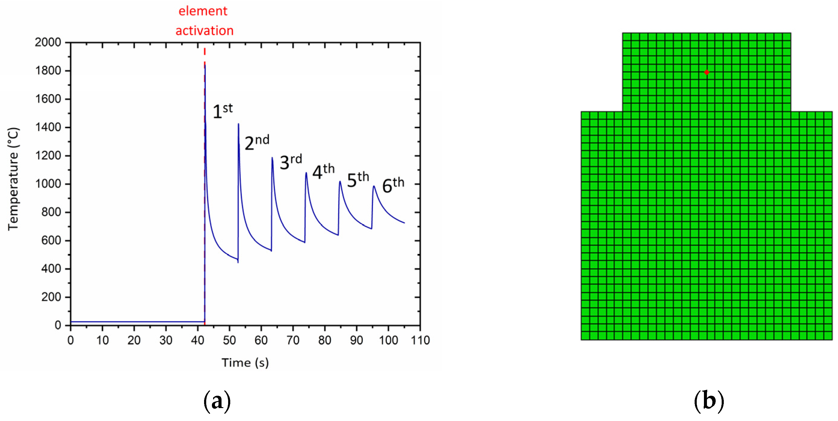
2.1. Thermal Analysis

In the present work, heat transfer calculations were performed using the ABAQUS finite element software [2]. The following formulation applies to solid body heat conduction with temperature-dependent conductivity, internal energy (including latent heat effects), and convection and radiation boundary conditions. The energy balance is given by

$$\begin{gathered} {\displaystyle \underset{\Omega }{\int }\rho \dot{U}dV}={\displaystyle \underset{\partial \Omega }{\int }-q\cdot ndS}+{\displaystyle \underset{\Omega }{\int }\rho \dot{r}dV}\forall \Omega \Rightarrow {\displaystyle \underset{\Omega }{\int }\left(\rho \dot{U}+\nabla \cdot q-\rho \dot{r}\right)dV}=0\forall \Omega \\ \rho \dot{U}+\nabla \cdot q-\rho r=0 \end{gathered}$$

(1)

where $\Omega$ is the space occupied by the material, $\partial \Omega$ the boundary of $\Omega$, $\rho$ the mass density of the material $\left(\mathrm{kg}/{\mathrm{m}}^3\right)$, $U$ the internal energy per unit mass $\left(\mathrm{J}/\mathrm{kg}\right)$, $q$ the heat flux per unit area $\left(\mathrm{W}/{\mathrm{m}}^2\right)$, $n$ the outward unit normal to $\partial \Omega$, $r$ the internal heat generation rate per unit volume $\left(\mathrm{J}/\mathrm{kg}\right)$, and a superposed dot denotes the material time derivative. Equation (1) is usually written in terms of specific heat $c\left(T\right)=\partial U\left(T\right)/\partial T$$\left(\mathrm{J}/\left(\mathrm{kg}{ }^{\mathrm{o}}\mathrm{C}\right)\right)$, where $T$ is temperature, so that

$$\dot{U}=\frac{\partial U\left(T\right)}{\partial T}\dot{T}=c\dot{T}$$

(2)

Heat conduction is assumed to be governed by the isotropic Fourier law

$$q=-k\cdot \nabla T$$

(3)

where $k$ is the temperature-dependent thermal conductivity tensor $\left(\mathrm{W}/\left(\mathrm{m}{ }^{\mathrm{o}}\mathrm{C}\right)\right)$. Combining Equations (1)–(3), we arrive at the governing equation for transient heat transfer analysis

$$\nabla \cdot \left(k\cdot \nabla T\right)+\rho \dot{r}=\rho c\dot{T}$$

(4)

when the material changes phase (e.g., melting or solidification), there is an additional change in the internal energy ${\dot{U}}_{\ell }$ (“latent heat effect”). In this case, we write

$$\nabla \cdot \left(k\cdot \nabla T\right)+\rho \left(\dot{r}-{\dot{U}}_{\ell }\right)=\rho c\dot{T}$$

(5)

where ${\dot{U}}_{\ell }>0$ in melting (material absorbs energy) and ${\dot{U}}_{\ell }<0$ in solidification (material releases energy). It is assumed that latent heat $U_{\mathrm{Latent}}$ is absorbed or released over a range of temperatures from a lower (solidus) temperature $T_s$ to an upper (liquidus) temperature $T_L$.

$$U_{\mathrm{Latent}}=U_{\ell }\left(T_L\right)-U_{\ell }\left(T_S\right)$$

(6)

The internal energy per unit mass associated to latent heat $U_{\ell }\left(T\right)$ is assumed to vary smoothly from $U_{\ell }\left(T_s\right)=0$ to $U_{\ell }\left(T_L\right)=U_{\mathrm{Latent}}$ as follows [3]:

$$U_{\ell }\left(T\right)=U_{\mathrm{Latent}}\left[3{\left(\frac{T-T_S}{T_L-T_S}\right)}^2-2{\left(\frac{T-T_S}{T_L-T_S}\right)}^3\right]$$

(7)

where the cubic function above is chosen so that ${\left(d{U}_{\ell }/dT\right)|}_{T=T_S}={\left(d{U}_{\ell }/dT\right)|}_{T=T_L}=0$.

Heat losses due to convection and radiation are specified as boundary conditions

$$q\cdot n=-h\left(T-T_0\right)-\sigma \epsilon \left[{\left(T-T_Z\right)}^4-{\left(T_0-T_Z\right)}^4\right]$$

(8)

where $h$ is the film coefficient $\mathrm{W}/\left({\mathrm{m}}^2{}^{\circ }\mathrm{C}\right)$, $T_0$ the sink temperature, $T_{\mathrm{z}}$ the absolute zero temperature, $\epsilon$ the emissivity (dimensionless), and σ = 5.669 × 10⁻⁸ W/(m² °C⁴) the Stefan–Boltzmann constant.

The material deposition in additive manufacturing is modeled by using “quiet” elements which are activated as the added material solidifies. In this approach, the elements are present in the analysis but are assigned properties, so they do not affect the analysis [4].

For heat transfer analyses, the material is assumed isotropic. The thermal conductivity $k$ and the specific heat $c$ are set to zero to minimize conduction and to adjust energy transfer to the quiet elements

$$k_{quiet}=0\mathrm{and}{c}_{quiet}=0$$

(9)

The laser beam was modeled as a heat source. In particular, the double ellipsoid volumetric source heat input model is used to simulate the heat input onto the part [5]:

$$\rho \dot{r}=\frac{6P}{\pi abc}\exp \left[-3\left(\frac{{\xi }^2}{a^2}+\frac{{\eta }^2}{b^2}\right)\right]$$

(10)

where $r$ is the heat supplied internally into the body per unit volume, $P=195\mathrm{W}$ the energy input rate, ($a=1.5\mathrm{mm}$, $b=0.9\mathrm{mm}$, $c=1\mathrm{mm}$) the semi-axis of the ellipsoid, and $\left(\xi ,\eta ,\zeta \right)$ the local coordinates at the ellipsoid center.

The heat source of the laser beam, the latent heat effects, as well as the heat losses due to convection and radiation were modeled via a “user subroutine” (DFLUX) in ABAQUS.

2.2. Microstructural Analysis

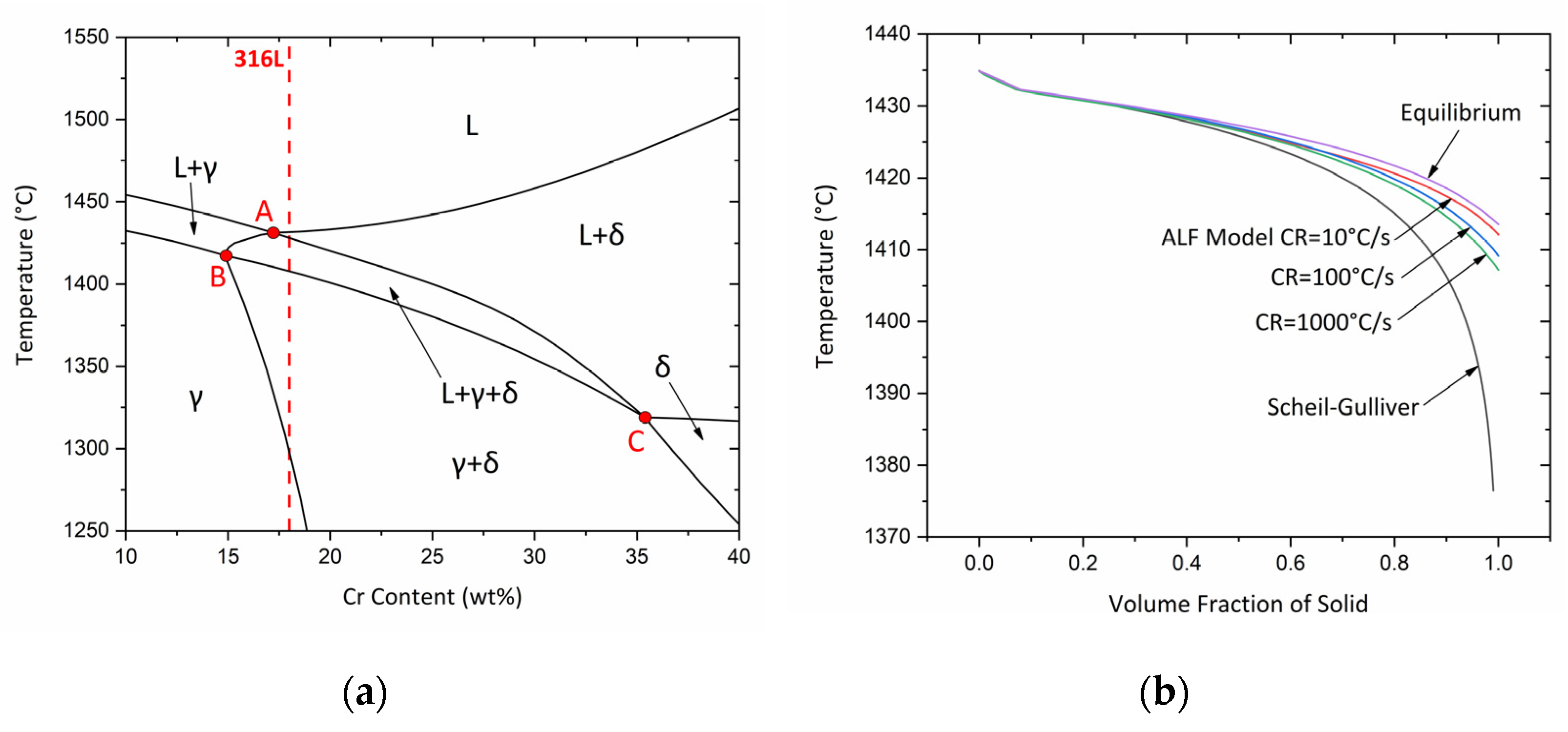
2.2.1. Thermodynamic Analysis

Computational alloy thermodynamics, based on the CALPHAD approach [6], were employed to describe the phase fractions at equilibrium conditions as well as the driving forces for phase transformations, in an austenitic stainless steel with nominal composition of Fe-18Cr-14Ni-2.6Mo-1Mn-0.03C (in wt%). All thermodynamic calculations were performed in the Thermo-Calc software [7] coupled with the TCFE6 thermodynamic database for ferrous alloys. A section of the phase diagram with respect to Cr (isopleth) was computed, revealing the solidification tie triangle, where the liquid phase (L), primary austenite (γ) phase, and primary ferrite (δ) phase coexist at equilibrium. The tie triangle is commonly present in austenitic stainless steels at elevated temperatures and the type of solidification is determined based on the solidification path relative to the corners of the triangle. The limiting case of equilibrium solidification provides useful information regarding the behavior of the system upon solidification and is the basis for the following calculations.

To better describe the non-equilibrium solidification phenomena, resulting from rapid heating and cooling, upon AM processes, the Scheil–Gulliver model was employed, as implemented in Thermo-Calc. Scheil–Gulliver simulations consider the extreme case of near-infinite colling rates, assuming that no diffusion occurs in the solid phases, the liquid has a homogeneous composition and that local equilibrium conditions are established on the solid/liquid interface, at all times during solidification.

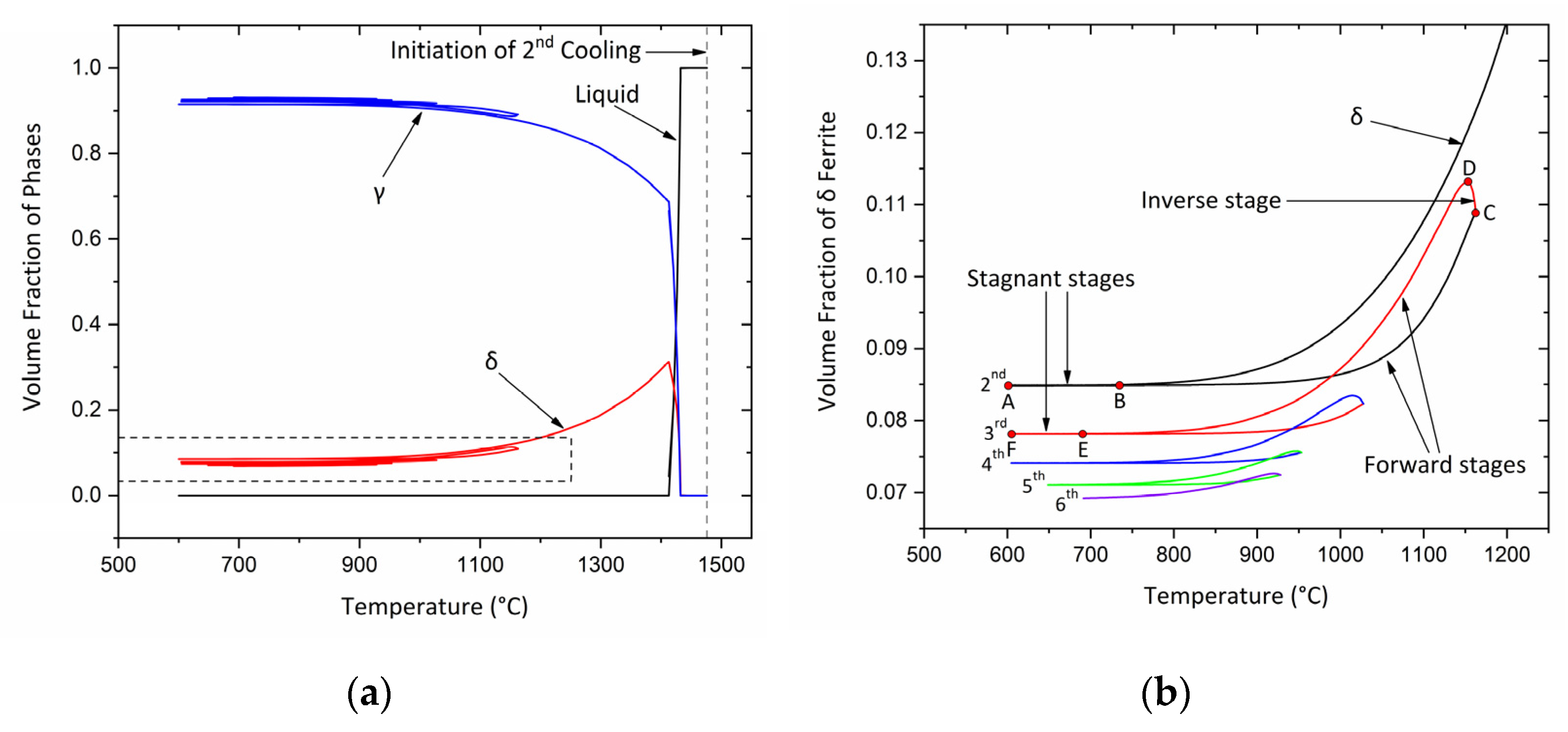
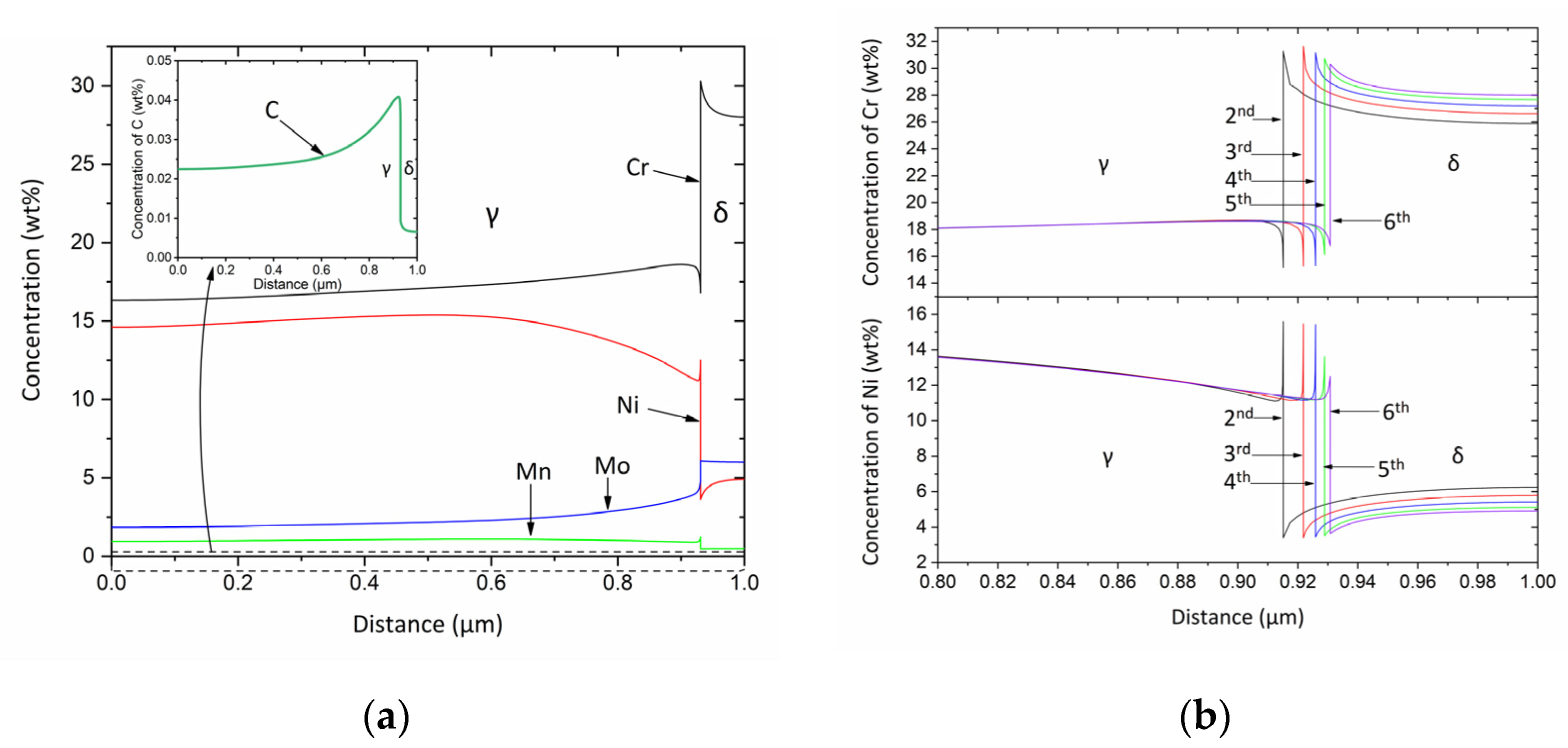
2.2.2. Diffusion Analysis

The equilibrium solidification and the Scheil–Gulliver models provide a fast and reliable method of determining the key phenomena and microstructural features during solidification. However, they both lack in the fidelity required to capture the interactions from subsequent heating and cooling cycles, as well as the spatial and temporal evolution of microstructural features, upon AM processing. Consequently, an in-depth analysis of solidification and solid phase transformations was conducted, considering the entire thermal cycle, as calculated by heat transfer simulations, by employing multicomponent and multiphase diffusion simulations [1]. Kinetic calculations were performed in the DICTRA module of Thermo-Calc [7], coupled with the MOBFE2 mobility and TCFE6 thermodynamic database. One-dimensional mass diffusion was considered in a planar geometry diffusion cell, with a size of 1μm, representative of the as-solidified microstructure. The cell is initially comprised of a single liquid phase region with two inactive regions of γ austenite and δ ferrite adjacent to it, separated via moving interfaces. As the temperature decreases and the inactive phases become thermodynamically stable, they nucleate and grow, consuming the liquid. The positioning of the austenite and ferrite regions compared to the liquid region allows for modeling of either eutectic or peritectic reactions. Eutectic solidification is simulated by positioning the austenite and ferrite regions of each side of the liquid as γ/L/δ, from now on referred to as ALF model. By positioning the austenite and ferrite phases adjacent to each other and the liquid as L/γ/δ, the LAF model is obtained, simulating the peritectic reaction. The present study focuses only on the ALF model for eutectic solidification, in the interest of simplicity, although the peritectic model can be considered as well, if suggested by experimental findings.

The kinetic simulations for the evolution of the microstructure were performed considering the thermal cycle of a selected point in the middle of the specimen, as determined via heat transfer simulations described in Section 2.1. It was observed that the second heating cycle, due to the subsequent material deposition and laser pass, resulted in a complete remelting of the solidified microstructure. Additional laser passes did not result in melting in the examined point. Therefore, the first cycle (laser pass) was omitted in the solidification analysis and the thermal profile from the second pass to the end of the process was considered. At low temperatures below 600 °C diffusion is sluggish and thus the phase fractions and the composition profiles remain relatively stagnant. However, significant numerical difficulties arise when integrating the diffusion equations, as the temperature decreases. For that reason, temperature sections laying lower than 600 °C, were replaced with an isothermal holding at 600 °C. Results using this simplified approach yielded no significant difference from the full approach, although they drastically decreased computational times. The kinetic analysis allows for the determination of spatial and temporal evolution of phase fractions and compositions, the presence of elemental microsegregation and the quantification of the freezing range, which are essential for the properties of the final product and could provide feedback for a following mechanical analysis.

3. Results and Discussion

3.1. Thermal Analysis Results

Based on the formulation described in Section 2.1, a thermal analysis using diffusive heat transfer elements (DC2D4) was performed in order to evaluate the temperature evolution in the processed part, due to the successive material deposition. In the present work, a two-dimensional wall is built, and a 15 mm × 14.5 mm substrate is used to start the metal deposition. The wall length is 10 mm and it is built by 10 layers of 0.5 mm height each. The substrate and wall model contains 1070 DC2D4 elements and 1162 nodes.

Each layer is generated by a single straight laser scan and the travel speed of the heat source is 20 mm/s. The idle time $\Delta t$ between the deposition of consecutive layers of material is set $\Delta t=10\mathrm{s}$. As mentioned in Section 2.1, the double ellipsoid volumetric source heat input model is used to simulate the heat input onto the part [5]. The values used here are $P=195\mathrm{W}$, $a=1.5\mathrm{mm},$ $b=0.9\mathrm{mm},$ and $c=1\mathrm{mm}$.

The free surface convection is set to $h=30\mathrm{W}/\left({\mathrm{m}}^2{}^{\mathrm{o}}\mathrm{C}\right)$. The gas and powder flow near the heating zone is simulated as a forced convection $h=630\mathrm{W}/\left({\mathrm{m}}^2{}^{\mathrm{o}}\mathrm{C}\right)$. The emissivity for radiation is set to $\epsilon =0.5$ and sink temperature to ${{\rm T}}_o=27{}^{\mathrm{o}}\mathrm{C}$.

Material properties for 316L austenitic stainless steel are used. The thermal conductivity $k$ and specific heat $c$ are listed in

Table 1. Thermal properties of 316L austenitic stainless steel.

$\mathbf{Temperature}\left({}^{\mathrm{o}}\mathrm{C}\right)$	$\mathbf{Thermal}\mathbf{Conductivity}\left(\mathbf{W}/\left(\mathbf{m}{}^{\mathbf{o}}\mathbf{C}\right)\right)$	$\mathbf{Specific}\mathbf{Heat}\left(\mathbf{kJ}/\left(\mathbf{kg}{ }^{\mathbf{o}}\mathbf{C}\right)\right)$
26.85	13.96	0.498
226.85	17.1	0.525
426.85	20.25	0.551
626.85	23.39	0.578
826.85	26.53	0.605
1026.85	29.67	0.631
1226.85	32.82	0.658
1526.85	35.96	0.684
1726.85	18.31	0.769
1926.85	18.97	0.769
2126.85	19.62	0.769
2326.85	20.28	0.769
2426.85	20.61	0.769

[8]. Material properties are linearly interpolated between the values listed on the table and kept constant beyond the minimum and maximum listed values. The density is $\rho =8030{\mathrm{kg}/\mathrm{m}}^3$. The latent heat of fusion $330\mathrm{kJ}/\mathrm{kg}$ and is spread over a temperature range from $1400{}^{\mathrm{o}}\mathrm{C}$ to $1459{}^{\mathrm{o}}\mathrm{C}$.

Figure 1a shows the temperature “history” of a selected material point. The solid part and substrate geometry employed in the thermal analysis and the selected material point, denoted by a red dot, are depicted in Figure 1b. The history of the temperature field computed in the thermal analysis will be used to determine the microstructural evolution in the processed part.

3.2. Microstructural Analysis Results

The calculated Cr isopleth for constant content of alloying elements is depicted in Figure 2a, while the red dashed line indicates the Cr content (wt%) of the present AISI 316L steel. The tie triangle ABC corresponds to the three-phase eutectic triangle L+δ+γ in which the liquid (L), primary ferrite (δ), and primary austenite (γ) phases coexist. According to the thermodynamic calculations, the solidification path is L→L+δ→ L+γ+δ→γ+δ, which is characterized as Ferritic–Austenitic (FA) type of solidification since primary ferrite forms prior to austenite. The equilibrium freezing range, defined as the difference between the Liquidus and Solidus temperatures, is around 21 °C. In Figure 2b, the solidification paths with respect to temperature and fraction of solid are shown using the equilibrium and Scheil–Gulliver models and the ALF diffusion model at three different constant cooling rates (10, 100 and 1000 °C/s). The Scheil–Gulliver model resulted in the highest freezing range of 58.5 °C, whereas the equilibrium at the lowest. Accordingly, for the case of the ALF diffusion model, employed to simulate the eutectic reaction, increasing the cooling rate results in higher freezing range. For high cooling rates, the solidification path curve approaches the curves calculated by the Scheil–Gulliver model, while for low cooling rates, the solidification path and the freezing range approach the equilibrium solidification. Therefore, the cooling rate determines the width of the freezing range, and the results calculated by the ALF diffusion model are located between the results obtained by the equilibrium and the Scheil–Gulliver models [9].

The variation of the volume fraction of phases with respect to temperature is presented in Figure 3a, after employing the thermal history given in Figure 1a, in the ALF diffusion model. The dashed vertical line in Figure 3a denotes the initiation of cooling in the second thermal cycle, where a complete cycle is comprised of a cooling stage, followed by a reheating stage. It should be noted that heating in the second thermal cycle resulted in total remelting of the material and thus results regarding the first cycle can be omitted. Upon cooling in the second thermal cycle, the primary δ ferrite phase solidifies, followed by the primary γ austenite phase, consuming the liquid (L) phase. The growth rate of δ ferrite decreases with the formation of γ austenite, and when the liquid phase is totally consumed, the γ austenite grows at the expense of δ ferrite. Furthermore, hysteresis loops are formed in the volume fraction curves of both austenite and ferrite during subsequent thermal cycling. A magnified region, under the rectangular dashed area in Figure 3a, is depicted in Figure 3b corresponding to the evolution of the volume fraction of δ ferrite during thermal cycling. It is observed that upon heating in the second thermal cycle, the volume fraction of δ ferrite in part A-B remains constant, and then gradually increases in part B-C. Therefore, the parts A-B and B-C on the volume fraction curve are referred to as “stagnant” and “forward” stages, respectively [10]. During cooling in the third thermal cycle, the volume fraction of δ ferrite in part C-D continues to increase. The part C-D on the volume fraction curve corresponds to the “inverse” stage since the volume fraction proceeds in a direction opposite to the temperature change. Upon further cooling in the 3rd cycle, the volume fraction of δ ferrite in parts D-E and E-F evolves according to the forward and stagnant transformation, respectively. It is interesting to note that the volume fraction of δ ferrite at the end of the cooling at each successive thermal cycle decreases, which is in accordance with the temperature change of the thermal cycling shown in Figure 1a.

The concentration profiles of C, Mn, Cr, Ni and Mo with respect to distance in the diffusion cell calculated with the ALF model at the end of the thermal cycling (sixth pass) are depicted in Figure 4a. Partitioning of C, Mn and Ni from δ ferrite to γ austenite takes place during the thermal cycling. The opposite partitioning behavior is observed for Cr and Mo. Therefore, at the end of thermal cycling, on the left side of the interface, the γ austenite phase is enriched in C, Mn, and Ni, whereas at the right side of the interface δ ferrite is enriched in Cr and Mo. During the solidification, the liquid phase becomes enriched in alloying elements. However, due to the sluggish diffusion of the substitutional elements in the solid phases, microsegregation is observed in both austenite and ferrite at the end of thermal cycling. It should be noted that C does not exhibit a segregation profile in austenite and ferrite due to its higher diffusivity in these phases.

The concentration profiles of Cr and Ni with respect to distance at the end of cooling after each successive thermal cycle are shown in Figure 4b. It is observed that the width of both Cr and Ni segregation profiles decreases at each thermal cycle, indicating that the concentrations of Cr and Ni in austenite and ferrite become homogeneous with the passage of time as diffusion takes place. In addition, the γ/δ interface is being displaced to the right by the end of each cooling cycle, resulting in the gradual decrease of the δ ferrite volume fraction, as equilibrium conditions are approached. Additionally, the concentrations of Cr in ferrite and Ni in austenite, on the interface, decrease at the last thermal cycles, following the local equilibrium conditions.

4. Conclusions

A thermal analysis was performed to simulate the thermal history during AM in a 316L stainless steel, followed by a microstructural analysis consisting of thermodynamic and kinetic calculations to describe the spatial and temporal evolution of phase fractions and compositions, as well as the freezing range and the elemental microsegregation upon solidification and thermal cycling. Two extreme cases of equilibrium and non-equilibrium solidification were analyzed after performing thermodynamic equilibrium calculations and using the Scheil–Gulliver model. Kinetic calculations were also performed to include the effect of multicomponent diffusion during eutectic solidification, after considering the entire thermal cycle as determined via heat transfer simulations.

According to thermodynamic and kinetic calculations, the cooling rate upon solidification determines the width of the freezing range, with the Scheil–Gulliver and the equilibrium solidification models resulting in the highest and lowest freezing ranges, respectively. Microsegregation of the substitutional elements is observed in austenite and ferrite phases during the thermal cycling from successive material deposition, while the width of the segregation profiles decreases at each cycle. The ensuing microstructural properties and the history of the temperature field computed in the thermal analysis can be used subsequently as input to the mechanical problem for the determination of the residual stress field, where the local mechanical properties could be estimated by using non-linear homogenization methods.

References

1. Sotiriou, M.P.; Tzini, M.I.T.; Aristeidakis, J.S.; Haidemenopoulos, G.N.; Barsoum, I. A computational study of solidification during additive manufacturing of AISI 304 austenitic stainless steel. In Proceedings of the 7th Panhellenic Conference on Metallic Materials, Athens, Greece, 11–13 December 2019. [Google Scholar]
2. Hibbitt, H.D. ABAQUS/EPGEN—A general purpose finite element code with emphasis on nonlinear applications. Nucl. Eng. Des. 1984, 77, 271–297. [Google Scholar] [CrossRef]
3. Spyrou, L.A.; Aravas, N. Thermomechanical Modeling of Laser Spot Welded Solar Absorbers. J. Manuf. Sci. Eng. 2015, 137, 1–16. [Google Scholar] [CrossRef]
4. Michaleris, P. Modeling metal deposition in heat transfer analyses of additive manufacturing processes. Finite Elem. Anal. Des. 2014, 86, 51–60. [Google Scholar] [CrossRef]
5. Goldak, J.; Chakravarti, A.; Bibby, M. A new finite element model for welding heat sources. Metall. Trans. B 1984, 15, 299–305. [Google Scholar] [CrossRef]
6. Lukas, H.L.; Fries, S.G.; Sundman, B. Computational Thermodynamics: The Calphad Method; Cambridge University Press: Cambridge, 2007; Volume 9780521868, ISBN 9780511804137. [Google Scholar]
7. Andersson, J.O.; Helander, T.; Höglund, L.; Shi, P.; Sundman, B. THERMO-CALC & DICTRA, Computational Tools For Materials Science. Calphad 2002, 26, 273–312. [Google Scholar] [CrossRef]
8. Kim, C.S. Thermophysical Properties of Stainless Steels; Argonne, IL, USA, 1975. [Google Scholar] [CrossRef]
9. Ohsasa, K.; Narita, T.; Nakaue, S.; Kudoh, M. Analysis of Solidification Path of Fe-Cr-Ni Ternary Alloy. ISIJ Int. 1995, 35, 629–636. [Google Scholar] [CrossRef]
10. Tzini, M.-I.; Sarafoglou, P.; Stieben, A.; Haidemenopoulos, G.; Bleck, W. Austenite Evolution and Solute Partitioning during Thermal Cycling in the Intercritical Range of a Medium-Mn Steel. Steel Res. Int. 2016, 87, 1686–1693. [Google Scholar] [CrossRef]
Figure 1. (a) Temperature history of a selected material point. (b) Solid part and substrate geometry employed in the thermal analysis. The red dot corresponds to the selected material point.
Materproc 03 00020 g001
Figure 2. (a) Isopleth of Cr for constant alloying elements composition at thermodynamic equilibrium. (b) Solidifications paths calculated by the Scheil–Gulliver and the multicomponent diffusion models.
Materproc 03 00020 g002
Figure 3. (a) Variation of the volume fraction of phases with respect to temperature. (b) Magnified region depicting the evolution of the volume fraction of δ ferrite during the thermal cycling.
Materproc 03 00020 g003
Figure 4. (a) Concentration profiles of C, Mn, Cr, Ni and Mo at the end of the thermal cycling. (b) Concentration profiles of Cr and Ni at the end of the cooling at each thermal cycle. The austenite and ferrite regions are on the left and right of the interface, respectively.
Materproc 03 00020 g004