Application and Evaluation of Surrogate Models for Radiation Source Search

Abstract

Surrogate models are increasingly required for applications in which first-principles simulation models are prohibitively expensive to employ for uncertainty analysis, design, or control. They can also be used to approximate models whose discontinuous derivatives preclude the use of gradient-based optimization or data assimilation algorithms. We consider the problem of inferring the 2D location and intensity of a radiation source in an urban environment using a ray-tracing model based on Boltzmann transport theory. Whereas the code implementing this model is relatively efficient, extension to 3D Monte Carlo transport simulations precludes subsequent Bayesian inference to infer source locations, which typically requires thousands to millions of simulations. Additionally, the resulting likelihood exhibits discontinuous derivatives due to the presence of buildings. To address these issues, we discuss the construction of surrogate models for optimization, Bayesian inference, and uncertainty propagation. Specifically, we consider surrogate models based on Legendre polynomials, multivariate adaptive regression splines, radial basis functions, Gaussian processes, and neural networks. We detail strategies for computing training points and discuss the merits and deficits of each method.

1. Introduction

Significant attention has been focused on accurate and efficient determination of the location of radioactive materials. This is especially important in urban environments, which are particularly susceptible to threats due to high population density. One strategy is to deploy a network of detectors, which count ionizing gamma rays that reach their location. The resulting problem is to locate a radioactive source in a complicated domain using this noisy detector data. The difficulties are compounded when the signal-to-background radiation ratios are low, which is often the case. One avenue of current research has focused on fusing detector data to determine the source location while attempting to decrease the number of detectors, increase the accuracy of the location estimate, and increase the efficiency of the algorithm [1,2,3]. This problem requires modeling the paths of the gamma particles emitted by the source by employing the Boltzmann transport equation to determine the origination location. Two standard methods for numerically solving the Boltzmann transport equation are to solve for the explicit, deterministic solution and the implicit, stochastic solution using Monte Carlo simulations of many particle histories. However, both are computationally expensive.

In prior work [2], we employed a 2D ray-tracing algorithm to model detector responses to a radiation source in a simulated city block. We used the open source code gefry to solve for the detector responses within this test environment [4]. Whereas this algorithm is based on Boltzmann transport theory, scattering is neglected to significantly improve the efficiency. It is shown in Ref. [5] that, despite these simplifying assumptions, the code can resolve source locations to within meters for the considered geometry and background levels. To solve the source localization problem, we employ Bayesian inference by using a Delayed Rejection Adaptive Metropolis (DRAM) algorithm [6], which requires thousands to millions of model evaluations to infer the 2D position $(x,y)$ and intensity I, which are the design variables used throughout this paper. Whereas the use of DRAM is tractable for this model, two issues motivate the construction of surrogate models: (1) extension to 3D models employing Monte Carlo N-Particle (MCNP) [7] simulations that incorporate more comprehensive physics; and (2) addressing the non-differentiable likelihood due to the presence of buildings in the geometry. We extend the analysis presented in Ref. [2] by exploring the choice of surrogate modeling technique and training point selection in this paper.

We performed preliminary research regarding the use of Monte Carlo simulations [7] to generate measurement data for nine point detectors in three dimensions with scattering in an extremely simplified geometry detailed in Ref. [8]. A Monte Carlo simulation was run once to generate synthetic measurements, and calibration was then performed against the calculated detector responses using the ray-tracing model. In this geometry, four rectangular prisms in a 2 × 2 layout were considered in a 100 m × 100 m domain, each adjusted to have wall thicknesses of 0.5 m of concrete. Employing the ray-tracing model for the source localization problem for a 662 keV source placed 1 m above the ground, we were able to localize the source to within 5 m. This level of accuracy is sufficient in this large-space source search problem. However, it required several CPU hours of computation to generate one set of detector measurements employing MCNP code [7,8]. For a realistic 3D geometry, such as a 3D version of the geometry depicted in Figure 1, thousands of CPU hours would be required to solve the source localization problem using only Monte Carlo simulations.

Furthermore, the model solution to the 2D problem exhibits discontinuous derivatives due to the buildings in the geometry, which block radiation paths to detectors. Hence, gradient-based sensitivity analysis and optimization are not directly applicable. Gradient free sensitivity analysis and optimization methods can be employed as done in prior work [2], which employs gradient free optimization methods for this problem, however another option is to develop differentiable surrogate models. To avoid similar difficulties in various non-differentiable models, studies have employed differentiable surrogate models for applications in reactor simulations [9], hydrology [10], and for use in general optimization strategies [11,12,13] and optimal design [14].

Similarly, we address these difficulties by investigating various differentiable surrogate models that approximate model solutions, which quantify detector responses, with suitable accuracy at a fraction of the computational expense. We employ spectral expansions using Legendre polynomials and radial basis functions as bases to generate two surrogate models. We explore several approaches to solving for the spectral expansion coefficients and compare interpolation and regression approaches. We also illustrate surrogate models based on multivariate adaptive regression splines (MARS), Gaussian processes (GP), and neural networks. We describe and compare the accuracy and efficiency of each surrogate model. In addition, we consider the choice of training points for surrogate model construction by comparing Gauss–Legendre points with Clenshaw–Curtis points, Latin hypercube sampling, and random sampling. Lastly, we test the Gaussian processes surrogate model by employing it in solving the source localization problem using DRAM [6].

This paper is organized as follows. In Section 2, we introduce the physical model, which we approximate with the surrogate models. In Section 3, we introduce each surrogate model and discuss its implementation. The choice of training points for the surrogate models is discussed in Section 4. In Section 5, we plot each surrogate model against the physical model evaluations to illustrate goodness of fit, we plot the relative root mean squared error ($rRMSE$) of the surrogate models, and we discuss and compare the performance of the surrogate models. To verify the surrogate response, we employ the Gaussian processes surrogate model to solve the source localization problem and compare it with the results from employing the ray-tracing model in Section 6. Lastly, in Section 7, we draw conclusions and present future work.

2. Physical Model

The problem of determining the location and intensity of a radiation source from detector measurements requires the solution of the Boltzmann equation describing the transport of neutral particles—i.e., particles with no electrical charge—which is computationally intractable to solve in real time. To address this problem, we make the assumption that gamma rays that suffer collisions before reaching a detector are never detected. Under this assumption, we obtain the model

$$\Omega ·\nabla \psi (r,E,\Omega )+\frac{1}{{\lambda }_T(r,E,\Omega )}\psi (r,E,\Omega )=\frac{I_0}{4\pi }\delta (E-E_0)\delta (||r-r_S{\left|\right|}_2)$$

(1)

describing gamma transport [15]. Here, $\psi$ denotes gamma intensity per unit area—particle scalar flux—at location r and $I_0$ denotes the intensity of the source, which is located at the position $r_S$ and emits gamma particles with directional unit vector $\Omega$ and energy E. The Dirac density $\delta (·)$ on the right-hand side isolates the source energy and position to $E_0,r_S$. Finally, ${\lambda }_T$ is the mean-free path, which is the mean distance traveled between collisions.

Solving Equation (1) for total flux at a certain point $r_i$, which we take to be the location of the ith detector, yields

$${\widehat{u}}_i\left(q\right)=I_0\Delta t_i{ϵ}_i\frac{A_i}{4\pi \left|\right|r_i-r_S{\left|\right|}_2^2}\exp \left(-{\int }_{r_S\to r_i}\frac{1}{{\lambda }_T}dr\right),i=1,\dots ,d,$$

(2)

where u is the expected number of gammas observed by a detector at location $r_i$, given the parameters $q=[r_S,I_0]\in \Omega$ corresponding to the source location, $r_S=(x_0,y_0)$ and intensity, $I_0$. Here, the path of the gammas from the source to the detector is represented by $r_S\to r_i$, which represents an arbitrary parameterization of the curve from $r_S$ to $r_i$; e.g., $[r_S\to r_i]\left(\tau \right)=r_S+(r_i-r_S)\tau$ where $\tau \in [0,1]$. Here, the ith detector has face area $A_i$, a dwell time $\Delta t_i$, and efficiency ${ϵ}_i$. The full derivation of this equation is provided in Ref. [5].

2.1. Numerical Model

We employ a ray-tracing scheme to determine the intensity of gammas reaching each detector at location $r_i$. For each detector, we construct a ray from the detector location to the source location. We compute the number of intersections with the $\mathcal{N}$ buildings, and the length ${\ell }_h$ of the ray segment through each of the $h=1,\dots ,\mathcal{N}$ buildings. The buildings in the domain are assumed to be homogeneous, each having a mean free path ${\lambda }_T^h,h=1,\dots ,\mathcal{N}$ [2]. These assumptions yield

$${\widehat{u}}_i\left(q\right)=I_0\Delta t_i{ϵ}_i\frac{A_i}{4\pi \left|\right|r_i-r_S{\left|\right|}_2^2}\exp \left(-\sum _{h=1}^{\mathcal{N}}\frac{{\ell }_h}{{\lambda }_T^h}\right),i=1,\dots ,d.$$

(3)

We employ the Python code gefry [4] to implement this numerical model, which is a significant simplification of the original problem derived from Boltzmann transport theory. Even so, because of the buildings in the geometry, this model is non-smooth and any extension of this model—to 3D or considering particle scattering–would yield a model that is computationally infeasible for Bayesian inference and uncertainty propagation.

2.2. Model Geometry

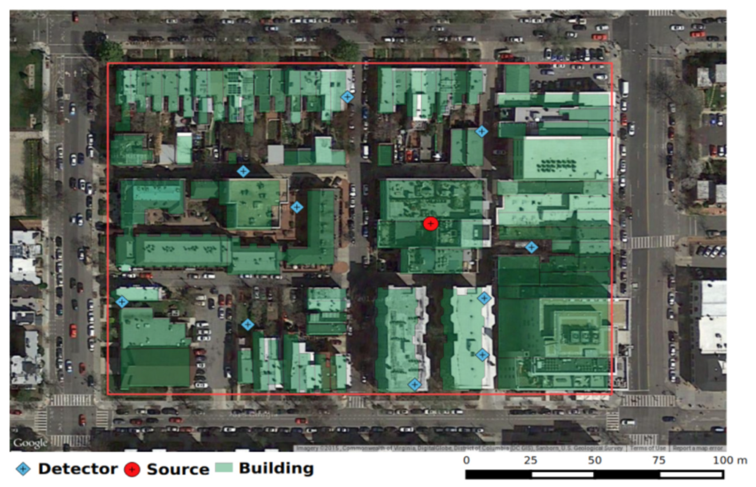
To apply and test this numerical model for a realistic scenario, we select the domain to be a $250\mathrm{m}\times 180\mathrm{m}$ block in downtown Washington, D.C. [2,5]. We construct a 2D representation of the domain using data from the OpenStreetMaps database. We treat the buildings as disjoint polygons of uniform density and composition, which define their individual macroscopic cross-sections. A satellite photo with the cross-sections overlaid is provided in Figure 1.

We semi-randomly assign each building an optical thickness between one and five mean free paths, with the larger and more dense buildings having larger optical thicknesses. This is motivated by an approximation that the wood and concrete buildings in this domain would have an average optical thickness of three mean free paths. We generate the detector locations, plotted as diamond marks in Figure 1, by sampling from a uniform distribution across the domain while excluding the walls of the buildings. We assume the detectors have facial areas $A_i=0.0058{\mathrm{m}}^2$ associated with three-inch diameters and three-inch lengths, intrinsic efficiencies of ${ϵ}_i=62\%$, and dwell times of $\Delta t_i=5$ s for $i=1,\dots ,10$. These efficiencies are typical for a standard NaI scintillator measuring 662 keV gamma particles. We use a background rate of $B=300$ counts per second, which is typical for this type of detector in an urban environment. In prior work [2], we showed that we are able to locate a source within the geometry despite these simplifications. Additionally, we are able to localize a source when building cross section uncertainties are increased as high as 50% of their nominal values [16].

2.3. Statistical Model

To develop surrogate models, we must first construct an appropriate statistical model. We assume a constant mean background with nominal intensity $B=300$ gamma counts per second and take $q_0=[x_0,y_0,I_0]$ to be the true source location and intensity. Radioactive decay and detection are Poisson random processes so we take the detector response to be a Poisson-distributed random variable. For each of the considered detectors, we employ the statistical model

$$Y_i=\mathrm{Pois}({\widehat{u}}_i\left(q_0\right)+B),i=1,\dots ,d,$$

(4)

for the total detector response. Here, $\mathrm{Pois}\left(\right)$ denotes the Poisson distribution with mean

$$u_i\left(q_0\right)={\widehat{u}}_i\left(q_0\right)+B,$$

(5)

for ${\widehat{u}}_i\left(q_0\right)$ given by Equation (3). The responses of d detectors are mutually independent. A Gaussian distribution approximates the Poisson distribution with a large expected value, which in this case is accurate for a large number of gamma observations. Therefore, we approximate Equation (4) by

$$Y_i\sim \mathcal{N}(u_i\left(q_0\right),{\sigma }_{0_i}^2),i=1,\dots ,d,$$

(6)

where ${\sigma }_{0_i}^2=u_i\left(q_0\right)={\widehat{u}}_i\left(q_0\right)+B$. We denote the detector observations by $y_i,i=1,\dots ,d$, which are realizations of the random variables

$$Y_i=u_i\left(q_0\right)+{ϵ}_i,i=1,\dots ,d,$$

(7)

where ${ϵ}_i\sim \mathcal{N}(0,{\sigma }_{0_i}^2)$.

3. Surrogate Models

Surrogate models are used to approximate input-output behavior of complex systems based on limited simulations [17]. For our application, we construct differentiable surrogate models, which approximate the non-differentiable ray-tracing model in Equation (3). These surrogate models are computationally feasible for use with 3D simulation codes or codes incorporating additional physics, such as photon scattering.

Whereas there are many methods to create surrogate models, we focus on response surface methods that treat the simulation code as a black box. This is one reason the surrogate modeling techniques we explore are feasible for use with high-fidelity codes. Two surrogate models are based on a polynomial expansion of the physical model evaluations using Legendre polynomials and radial basis functions. We employ discrete projections, which interpolate the data, to evaluate the Legendre polynomial surrogate models. To compare, we consider radial basis function surrogate models constructed using regression and a Legendre polynomial-based surrogate model constructed using sparsity-controlled regression for evaluation of the surrogate models. In addition, we consider a surrogate model based on a multivariate adaptive regression splines (MARS) algorithm. Finally, we demonstrate Gaussian processes and artificial neural networks for surrogate model construction.

Our strategy is to construct an individual surrogate model at each of the $d=10$ randomly chosen detector locations in the urban geometry. To compute the surrogate model response at source locations $(x,y)\in [0,250\mathrm{m}]\times [0,180\mathrm{m}]$ with intensities $I\in [5\times {10}^8,5\times {10}^{10}\mathrm{Bq}]$, we sample the mean response $u_i\left(q^m\right)$ at $M={21}^3=9261$ Gauss–Legendre training points $q^m\in \Omega =[0,250\mathrm{m}]\times [0,180\mathrm{m}]\times [5\times {10}^8,5\times {10}^{10}\mathrm{Bq}]$ for each of the $i=1,\dots ,d$ detector locations. Note that a Bequerel (Bq) is a unit of the activity of nuclear decay in a quantity of radioactive material per second. It takes 4.23 h to compute these 9261 model evaluations for each of the 10 detectors on a computer with a 3.4 GHz Intel core processor and 16 GB of memory. Whereas the computations can be parallelized, we report serial values in Section 5.

For each of the d detectors, we denote the surrogate model by $u_i^N,i=1,\dots ,d$, and relate it to the physical model solution $u_i={\widehat{u}}_i+B$ via the statistical model

$$\begin{array}{c}\hfill u_i^N\left(q^m\right)=u_i\left(q^m\right)+{\epsilon }_i^m,m=1,\dots ,M.\end{array}$$

(8)

The model discrepancies ${\epsilon }_i^m$ quantify unresolved fine-scale behavior incorporated in the ray-tracing model but neglected in the surrogate model. It is reasonable to assume that ${\epsilon }_i^m$ are identically distributed with variance ${\sigma }_0^2$, but one cannot justify the more stringent assumption that ${\epsilon }_i^m\sim \mathcal{N}(0,{\sigma }_0^2)$.

For all but neural networks, we can express surrogate models as

$$\begin{array}{c}\hfill u_i^N(q,w^i)=\sum _{j=1}^N{w}_j^i{\Psi }_j\left(q\right)+P_i\left(q\right),\end{array}$$

(9)

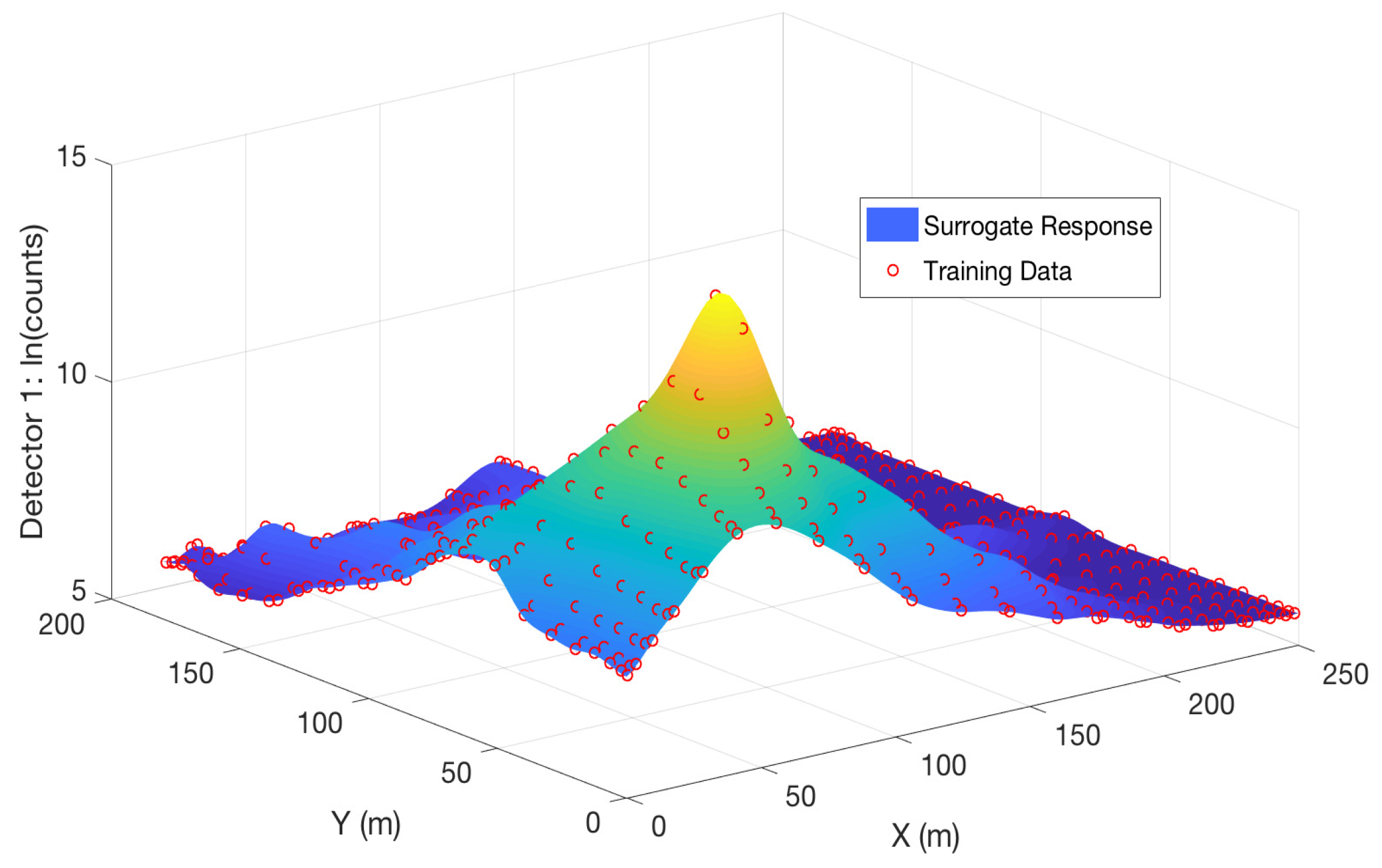
where $w^i=[w_1^i,\dots ,w_N^i]$ are coefficients and ${\Psi }_j\left(q\right)$ are basis functions that define the surrogate model. The trend functions $P_i\left(q\right)$ quantify global trends exhibited by the model. To demonstrate the goal of surrogate model construction, we plot a Gaussian process-based surrogate response surface versus the training points for a fixed intensity in Figure 2. We note that the detector response increases as the source is moved closer to the detector location and the response surface accurately quantifies the behavior of the training data. Additionally, we note that the surrogate model has smoothed the surface represented by the training data, most notably near the singularity at the detector location caused by the $\left|\right|r_i-r_S\left|\right|$ term in the denominator of Equation (3).

To verify each of the d models, we compare the surrogate and physical models at $S=500$ randomly generated test points $q^s\in \Omega$. The physical model takes 13.63 min to compute detector responses for the test points. We quantify errors by computing the relative root mean square error ($rRMSE$)

$$\begin{array}{c}\hfill rRMS{E}_i\equiv {\left[\frac{1}{S}\sum _{s=1}^S{\left(\frac{u_i\left(q^s\right)-u_i^N\left(q^s\right)}{u_i\left(q^s\right)}\right)}^2\right]}^{1/2}\end{array}$$

(10)

at each detector. Since the detector responses (in counts per second) vary over orders of magnitude, we compute the surrogate model responses based on the natural logarithm of the ray-tracing solution. For each surrogate model, we report $rRMSE={\sum }_{i=1}^d{\mathrm{rRMSE}}_i$ and plot the surrogate and physical model responses at the first 50 test points in Section 5. Whereas the surrogate and physical model responses at these test points are discrete, we plot the points continuously for clarity. Additionally, we plot the $rRMS{E}_i$ of each surrogate model for $i=1,\dots ,d$ for the $d=10$ detectors. We note that performance metrics such as proper scoring rule [18] or Mahalanobis distance can be employed to obtain some assessment of the uncertainty in the surrogate model, but we leave this as future work.

To minimize notation overload throughout the remaining discussion, we drop the dependence on i and express the surrogate and statistical models as

$$\begin{array}{c}\hfill u^N(q,w)=\sum _{j=1}^N{w}_j{\Psi }_j\left(q\right)+P\left(q\right),\end{array}$$

(11)

and

$$\begin{array}{c}\hfill y=u\left(q\right)=u^N(q,w)+\epsilon ,\end{array}$$

(12)

where we combine errors from the ray-tracing algorithm and surrogate model construction in $\epsilon$. However, we remind the readers that we construct individual surrogate models for each of the $i=1,\dots ,d$ detectors.

3.1. Legendre Polynomials

For polynomial interpolation and regression, we assume that the physical model responses can be expressed as

$$\begin{array}{c}\hfill u\left(q\right)=u(q,w)=\sum _{j=1}^{\infty }{w}_j{\Psi }_j\left(q\right),\end{array}$$

(13)

which we approximate to obtain the surrogate model

$$\begin{array}{c}\hfill u^N(q,w)=\sum _{j=1}^N{w}_j{\Psi }_j\left(q\right).\end{array}$$

(14)

We take ${\Psi }_j\left(q\right)$ to be multivariate Legendre polynomials—i.e., products of univariate Legendre polynomials—which are defined as the solution to the differential equation

$$\begin{array}{c}\hfill \frac{d}{dq}\left[(1-q^2)\frac{d}{dq}{\Psi }_j\left(q\right)\right]+j(j+1){\Psi }_j\left(q\right)=0.\end{array}$$

(15)

The first three univariate Legendre polynomials are

$$\begin{array}{cc}\hfill & {\Psi }_1\left(q\right)=1,\hfill \end{array}$$

(16)

$$\begin{array}{cc}\hfill & {\Psi }_2\left(q\right)=q,\hfill \end{array}$$

(17)

$$\begin{array}{cc}\hfill & {\Psi }_3\left(q\right)=\frac{1}{2}(3q^2-1)\hfill \end{array}$$

(18)

for $q\in \widehat{\Omega }=[-1,1]$. These polynomials are orthogonal on the interval $\widehat{\Omega }=[-1,1]$ with respect to the density $\rho \left(q\right)=\frac{1}{2}$. We note that the roots of the univariate Legendre polynomials provide the Gauss–Legendre training points, $q^m,m=1,\dots ,M$, that we use to construct the surrogate models.

An important feature of polynomial approximations is that their accuracy is improved for functions with more regularity. We have spectral convergence for Legendre polynomial expansions of functions on $[-1,1]$ with error bounds

$$\begin{array}{c}\hfill \left|\right|u(q,w)-u^N{(q,w)\left|\right|}_{L^2[-1,1]}\le C_k{N}^{-k}{\left|\right|u(q,w)\left|\right|}_{H^k\left([-1,1]\right)}.\end{array}$$

(19)

Here, $C_k\ge 0$ is a constant that may depend on k and $u\in H^k\left([-1,1]\right)$, where $H^k\left([-1,1]\right)$ is a Sobolev space of $L^2$ functions with weak derivatives of all orders up to k in $L^2$. We should observe the convergence rate $C{N}^{-1}{\left|\right|u(q,w)\left|\right|}_1$, since our model is continuous, but has non-continuous derivatives [19]. We observe a convergence rate of $rRMSE\left(u^N\right)/rRMSE\left(u^{N/2}\right)\approx 0.8$, where $rRMSE\left(u^N\right)$ means the relative root mean squared error defined in Equation (10) of the Legendre-polynomial-based surrogate model employing N basis functions. This is not the convergence rate of $rRMSE\left(u^N\right)/rRMSE\left(u^{N/2}\right)\approx 0.5$ that we expected to observe, since

$$\frac{C{N}^{-1}{\left|\right|u(q,w)\left|\right|}_1}{C{(N/2)}^{-1}{\left|\right|u(q,w)\left|\right|}_1}=\frac{N^{-1}}{{(N/2)}^{-1}}=\frac{1}{2}.$$

(20)

However, this rate is closer to $0.5$ for certain values of N, as can be seen in the convergence results in $rRMSE$ of the Legendre polynomials that we compile in

Table 1. Convergence of Legendre surrogate model $rRMSE$ as N increases.

N	2	4	8	16	32	64	128	256	512	1024	2024
rRMSE	1.598	1.382	1.113	0.825	0.633	0.468	0.387	0.331	0.281	0.236	0.213
$\frac{rRMSE\left(u^N\right)}{rRMSE\left(u^{N/2}\right)}$		0.865	0.805	0.741	0.767	0.739	0.827	0.855	0.849	0.840	0.903

. We also bound N from above to address overfitting the noise in the physical model response.

We consider two methods to solve for the coefficients $w_j$. The first is based on discrete projection, which exploits the orthogonality of the polynomials ${\Psi }_j\left(q\right)$ to interpolate the function of interest at $u\left(q^m\right),m=1,\dots ,M$; i.e., the physical model simulations defined in Equation (3). Multiplying both sides of Equation (13) by ${\Psi }_j\left(q\right)$ and integrating over $\widehat{\Omega }$, yields

$$\begin{array}{c}\hfill w_j=\frac{1}{{\gamma }_j}{\int }_{\widehat{\Omega }}u(q,w){\Psi }_j\left(q\right)\rho \left(q\right)dq,j=1,\dots ,N,\end{array}$$

(21)

by exploiting the orthogonality relation

$$\begin{array}{c}\hfill {\int }_{\widehat{\Omega }}{\Psi }_j\left(q\right){\Psi }_i\left(q\right)\rho \left(q\right)dq=\left\{\begin{array}{cc}0\hfill & \mathrm{for}i\ne j\hfill \\ {\gamma }_j\hfill & \mathrm{for}i=j.\hfill \end{array}\right.\end{array}$$

(22)

Here, ${\gamma }_j=\frac{2}{2j+1}$ is a normalization constant and $\rho \left(q\right)=\frac{1}{2}$ is the associated density over $\widehat{\Omega }=[-1,1]$.

We approximate this integral by a quadrature rule, such as Gauss–Legendre quadrature, to obtain the approximate relation

$$\begin{array}{c}\hfill w_j\approx \frac{1}{{\gamma }_j}\sum _{r=1}^{R}u\left(q^r\right){\Psi }_j\left(q^r\right)\rho \left(q^r\right){\omega }^r,j=1,\dots ,N\end{array}$$

(23)

for the coefficients of the surrogate model. Here, $q^r$ are the sampled inputs, ${\omega }^r$ are the quadrature weights, and $u\left(q\right)={\widehat{u}}_i\left(q\right)+B$, where ${\widehat{u}}_i\left(q\right)$ solves Equation (3) and we have dropped the dependence on w. We employ Gaussian quadrature, since with only $R+1$ training points, polynomials of degree less than or equal to $2R+1$ can be integrated exactly. We set $R=M$ and $N=\frac{(p+K)!}{p!K!}$, where p is the number of parameters—three in our case—and K is the maximum degree of the multivariate Legendre polynomials [17].

We construct the multivariate Legendre polynomials as tensor products of univariate Legendre polynomials. As discussed in Ref. [20], the surrogate model error decreases roughly exponentially with polynomial degree, provided that a high enough order quadrature rule is used; e.g., large R. However, results with high degree polynomials—large K—diverge because of large fluctuations in the function $u^N$ between the quadrature points produced by overfitting; i.e., $u^N$ begins fitting observation errors.

To determine the correct degree K, we compute the sum of squares (SSq) error of the surrogate model evaluated at the test points $q^s$

$$\begin{array}{c}\hfill SSq=\sum _{s=1}^S{[u\left(q^s\right)-u^N(q^s,w)]}^2,\end{array}$$

(24)

and compute the likelihood

$$\begin{array}{cc}\hfill & \pi \left(u\right|q)=\frac{1}{{\left(2\pi {\sigma }_0\right)}^{S/2}}{e}^{-SSq/2{\sigma }_0^2},\hfill \end{array}$$

(25)

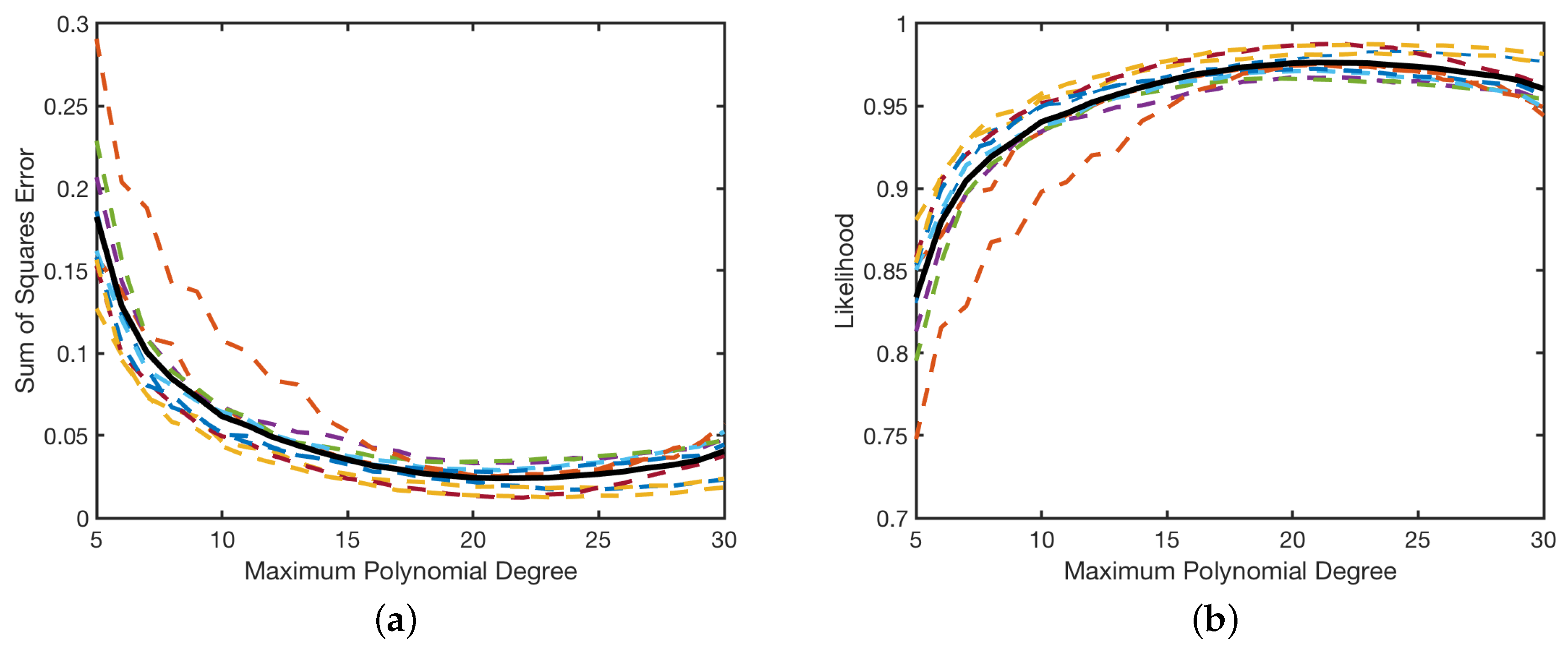
for the surrogate model $u^N$ with maximum polynomial degree $K=1,\dots ,30$. We plot the results in Figure 3, where the results for the $d=10$ surrogate models are plotted with the mean value overlaid in a thicker line. We see that the mean sum of squares error has a distinct minimum and the mean likelihood has a maximum at $K=21$. Hence, we use this value when computing the surrogate model and employ $N=2024$ total basis functions. Akaike information criteria (AIC), Bayesian information criteria (BIC), or cross validation techniques can also be employed to determine the value of K that balances accuracy versus overfitting of the surrogate model. These cross-validation procedures are discussed further in Ref. [21,22]. An alternative to using such a high degree polynomial for this surrogate model is to employ splines, which we consider in Section 3.2.

We note that these surrogate models, excluding the Gaussian processes surrogate model, are all parametric models. Whereas there are multiple definitions of parametric models, we define a parametric model as one where the class of basis functions is defined prior to construction of the model. Since we employ the class of Legendre polynomials to construct this surrogate model, we classify it as a parametric surrogate model. We classify Gaussian processes as semi-parametric under this definition, as is discussed in Section 3.4.

An alternate method to obtain the coefficients $w_j$ is to perform a least absolute shrinkage and selection operator (LASSO) regression [23]. Borrowing from compressive sensing (CS), we bound the $l_1$ norm of the coefficients to enforce sparsity. Therefore, we can formulate the problem as the optimization problem

$$\begin{array}{c}\hfill \underset{c}{min}\left|\right|\Lambda c-{y\left|\right|}_2^2{,\mathrm{subject}\mathrm{to}\left|\right|c\left|\right|}_1\le \tau ,\end{array}$$

(26)

where ${\Lambda }_{jm}={\Psi }_j\left(q^m\right)$ is a matrix of the Legendre basis functions, $y={[y^1,\dots ,y^M]}^T$ is the vector of observations obtained from the statistical model defined in Equation (12), and $c={[w_1,\dots ,w_N]}^T$ is the vector of coefficients. To solve this optimization problem, we use the MATLAB SPGL1 solver, which is detailed in Ref. [23].

We tested multiple values of $\tau$, but use $\tau =35$ to obtain the results discussed in Section 4 and Section 5. We determine this value of $\tau$ by computing the 1-norm of the coefficients obtained via discrete projection. We find that these coefficients have a 1-norm between 32 and 38, and, when we decrease $\tau$ below 32, significant error is introduced. When we increase $\tau$ to greater than 38, the 1-norm of the coefficients is less than $\tau$, meaning that the constraint has no effect on the problem. When comparing the coefficients between these two methods, we see that they are similar but not identical, even when $\tau >38$. Further analysis on determining optimal values of $\tau$ is discussed in Ref. [23].

3.2. Multivariate Adaptive Regression Splines

Multivariate Adaptive Regression Splines (MARS) were first proposed by [24] as a procedure for performing adaptive nonlinear regression using piecewise linear (spline) basis functions. MARS follows from recursive partitioning regression, which is also outlined in Ref. [24]. The MARS linear basis functions, often termed hinge functions, are introduced in pairs on either side of a “knot” t, where there is an inflection point in a particular parametric direction; e.g.,

$$\begin{array}{c}\hfill {\psi }_k\left(q\right)=\max (0,q_i-t)\mathrm{and}{\psi }_{k+1}\left(q\right)=\max (0,t-q_i)\end{array}$$

(27)

are introduced concurrently. Here, $q_i,i=1,\dots ,p$ denotes the ith component of q, where $p=3$ in our model, since $q=(x,y,I)$. In this way, the domain is divided so that ${\psi }_k\left(q\right)$ is zero for $q_i<t$ and ${\psi }_{k+1}\left(q\right)$ is zero for $q_i>t$.

We employ an adaptive regression algorithm to generate knot locations using data ${\{q^m,y^m\}}_{m=1}^M$ from the statistical model defined in Equation (12) for the 10 detectors. We take the knot locations to be $t\in {\left\{q_i^m\right\}}_{i=1,m=1}^{p,M}$. An additive MARS model would take the basis functions to be ${\Psi }_k\left(q\right)={\psi }_k\left(q\right)$, but we consider products of the linear basis functions, thus we take the basis functions to be

$$\begin{array}{c}\hfill {\Psi }_j\left(q\right)=\prod _{k=1}^{K_j}{\psi }_k\left(q\right)=\prod _{k=1}^{K_j}{\left[s_{jk}(q_{v(j,k)}-t_{jk})\right]}_{+}.\end{array}$$

(28)

Here, $v(j,k)\in \{1,\dots ,p\}$ labels the component of the parameter vector or “predictor variable” $q={\left\{q_i\right\}}_{i=1}^p$, $K_j\le p$ is the level of interaction between the linear basis functions, and $t_{jk}$ is the kth knot employed by the jth basis function. Furthermore, the positive subscript means take the maximum of zero and the argument, as in Equation (27), and we take ${\Psi }_0\left(q\right)=1$ and $s_{jk}=\pm 1$. For simplicity, we consider only piecewise linear basis functions $\psi \left(q\right)$, although this algorithm can also be performed with other piecewise basis functions, such as cubic. Additionally, we consider up to second-order interactions of the linear basis functions $\psi$; i.e., $K_j\le 2$, and first-order interactions of the linear basis functions that are a function of the same variable. We found that employing second-degree interactions—i.e., products of linear basis functions of the same variable—did not increase the performance of the surrogate models significantly.

The surrogate model is

$$\begin{array}{c}\hfill u^N(q,w)=\sum _{j=0}^N{w}_j{\Psi }_j\left(q\right),\end{array}$$

(29)

where ${\Psi }_0\left(q\right)=1$ and the coefficients $w_j$ are estimated using least-squares regression. Note that this is the same form as Equation (11), for $w_0=1$ and ${\Psi }_0\left(q\right)=P\left(q\right)$. The construction of the MARS model takes place in two steps. In the forward step, basis functions are added to the model to reduce a “lack of fit” value, which we take to be the least-squares error of the surrogate model to the physical model evaluated at the training points. This is performed until a user defined maximum number of terms is reached. The maximum number of terms we use in the forward process of the MARS algorithm to construct this surrogate model is $N=200$.

The MARS algorithm purposefully overfits the model to the data in its forward simulation and then performs a backward deletion strategy in the second step to remove basis functions that no longer contribute sufficiently to the accuracy of the model fit. This is performed via a model selection procedure employing Generalized Cross-Validation (GCV) to compare models with subsets of the basis functions. The GCV equation,

$$\begin{array}{c}\hfill GCV=\frac{\frac{1}{M}{\sum }_{m=1}^M{\left[y^m-u^N(q^m,w)\right]}^2}{{\left[1-\frac{N+\kappa \times (N-1)/2}{M}\right]}^2},\end{array}$$

(30)

is a goodness of fit test that uses the parameter $\kappa$ to penalize large numbers of basis functions N [25]. We use a default penalty parameter of $\kappa =3$ and a threshold value of $GCV<{10}^{-3}$, which is used as a stopping criterion for the backward phase. The suggested threshold value is ${10}^{-4}$ and should be reduced for noise free data.

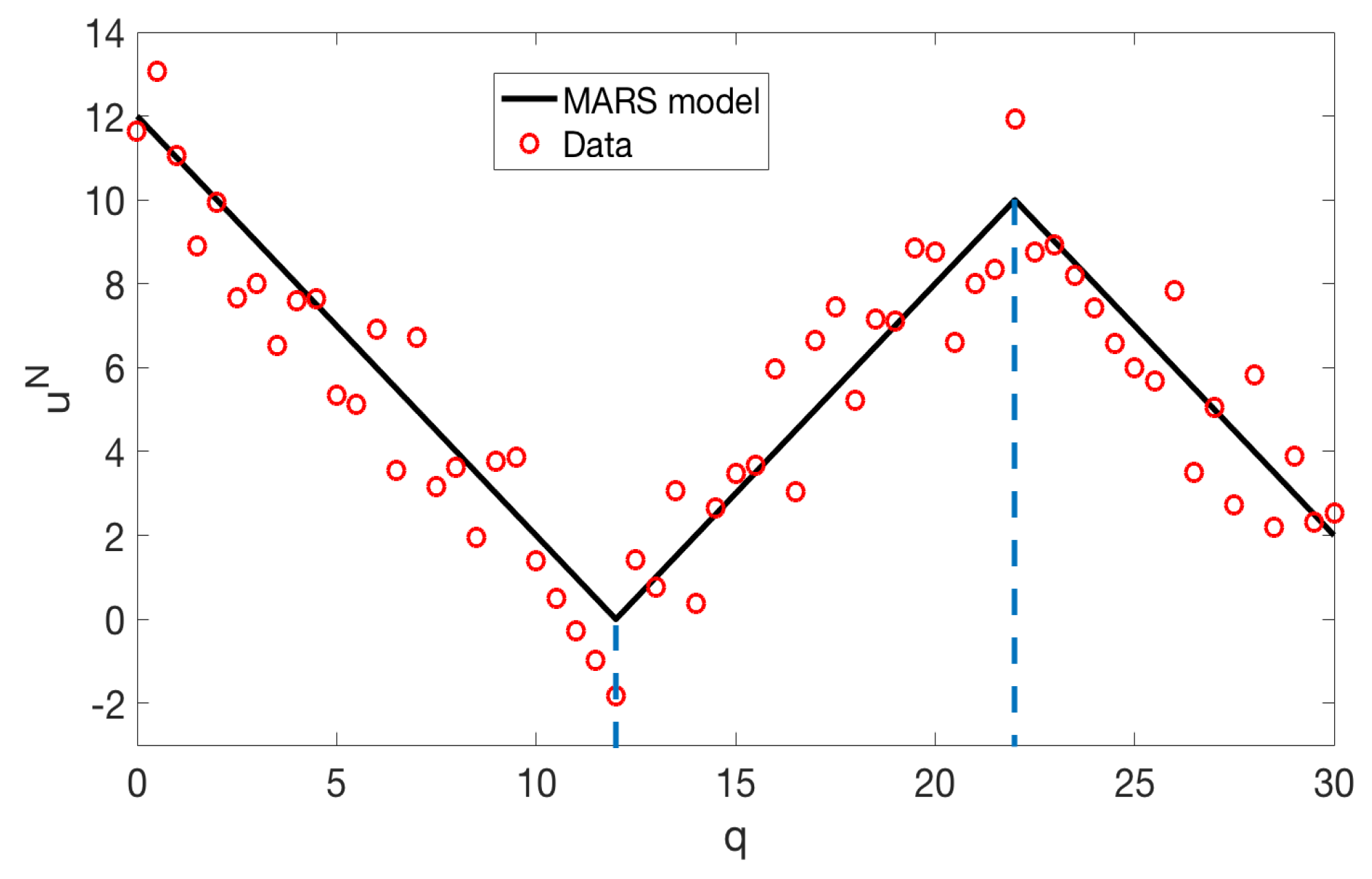
To better understand the MARS model structure, consider the problem of approximating the data depicted in Figure 4. We employ the MARS model

$$\begin{array}{c}\hfill u^N\left(q\right)=20-\max (q-12,0)+3\times \max (12-q,0)-2\times \max (22-q,0)\end{array}$$

(31)

to approximate the data. The knot locations at $q=12$ and $q=22$ delimit the regions where different linear relationships are identified. By considering the products of these linear basis functions, we can quantify nonlinear behaviors of the model.

To motivate error analysis of the MARS surrogate model, we consider the full MARS model

$$\begin{array}{c}\hfill u^N(q,w)=w_0+\sum _{j=1}^N{w}_j\prod _{k=1}^{K_j}{\left[s_{jk}(q_{v(j,k)}-t_{jk})\right]}_{+},\end{array}$$

(32)

where $w_0$ is the coefficient of the constant basis function. The sum is over the basis functions

$$\begin{array}{cc}\hfill B_i\left(q_i\right)& =\sum _{K_j=1}{w}_j{\Psi }_j\left(q_i\right)=\sum _{K_j=1}{w}_j{\left[s_{j1}(q_i-t_{j1})\right]}_{+},\mathrm{for}i\in V_j,\hfill \end{array}$$

(33)

$$\begin{array}{cc}\hfill B_{ik}(q_i,q_k)& =\sum _{K_j=2}{w}_j{\Psi }_j(q_i,q_k)=\sum _{K_j=2}{w}_j{\left[s_{j1}(q_i-t_{j1})\right]}_{+}{\left[s_{j2}(q_k-t_{j2})\right]}_{+},\mathrm{for}i,k\in V_j,\hfill \\ \hfill & ⋮\hfill \end{array}$$

(34)

where we now consider higher-order products of basis functions; i.e., $K_j\ge 1$. Here, $V_j={\left\{v(j,k)\right\}}_1^{K_j}$ is the set of predictor variable component labels for the jth basis function ${\Psi }_j$. Whereas this representation of the model does not provide insight into the model development, it allows us to rearrange the model in a way that reveals the predictive behavior of the model. By collecting basis functions that involve identical predictor variable sets, we obtain the representation

$$\begin{array}{c}\hfill u^N\left(q\right)=w_0+B_i\left(q_i\right)+B_{ik}(q_i,q_k)+B_{ik\ell }(q_i,q_k,q_{\ell })+\dots \end{array}$$

(35)

These sums represent the $K_j$ level interactions, if present, between the variables within the model. By adding the univariate contributions to the bivariate contributions, we obtain the representation

$$\begin{array}{c}\hfill B_{ik}^{*}(q_i,q_k)=B_i\left(q_i\right)+B_k\left(q_k\right)+B_{ik}(q_i,q_k).\end{array}$$

(36)

This provides a bivariate tensor product spline approximation representing the joint bivariate contributions of $q_i$ and $q_k$ to the model [24]. Similar rearranging can be performed by employing this representation combined with the trivariate functions to obtain the joint contributions of $q_i$, $q_k$, and $q_{\ell }$. Since Equation (35) is similar to analysis of variance decomposition [17], we refer to this as the ANOVA decomposition of the MARS model. The optimal additive approximation corresponds to the first-order terms in the ANOVA expansion, thus, if the higher-order indices are small, then the function can be approximated well by an additive model; i.e., $K_j=1,j=1,\dots ,N$. Note that, for our purposes, we consider a model with second-order interactions, thus we truncate Equation (35) at the second-order interactions. Unfortunately, the adaptivity of MARS makes it difficult to bound the error in the manner of spectral approaches that bound the error in terms of the coefficients $w_j$. However, cross validation procedures, such as those detailed in Ref. [21,22], can be used to provide an error estimate for the MARS model.

The MARS algorithm can be cast in a Bayesian framework in which case the number of basis functions N, their coefficients $w_j$, and their form—knot points $t_{jk}$, sign indicators $s_{jk}$, and the level of interaction $K_j$—are considered to be random [26]. Since any MARS model can be uniquely defined by these values, the Bayesian MARS model sets up a probability distribution over the space of possible MARS structures. The data are then used to infer these hyperparameters by employing a Markov chain Monte Carlo (MCMC) reversible jump simulation algorithm [27]. Currently, a form of this algorithm has been implemented in the R package BASS (Bayesian adaptive spline surface), but no such package exists for MATLAB. Hence, a comparison of BASS with these surrogate models is deferred to future research.

The MARS surrogate model takes advantage of the local low dimensionality of the function of interest, even if that function is strongly dependent on a large number of variables; i.e., large p. We employ the third-party ARESLab toolbox for MATLAB [28], which employs an algorithm similar to MARS [24]. Following the backward deletion step performed by this toolbox, the surrogate models discussed in Section 4 and Section 5 for each of the 10 detectors employ between $N=20$ and $N=36$ basis functions.

3.3. Radial Basis Functions

Here, we consider expansions

$$\begin{array}{c}\hfill u^N(q,w)=\sum _{j=1}^N{w}_j{\Psi }_j\left(q\right)\end{array}$$

(37)

with radial basis functions

$$\begin{array}{c}\hfill {\Psi }_j\left(q\right)=\Psi \left(\right||q-q^j{\left|\right|}_2)=\Psi \left(h_j\left(q\right)\right)\end{array}$$

(38)

defined in terms of the Euclidean distance

$$\begin{array}{c}\hfill h_j\left(q\right)=\left|\right|q-q^j{\left|\right|}_2={\left[\sum _{i=1}^p{(q_i-q_i^j)}^2\right]}^{1/2}.\end{array}$$

(39)

We remind the reader that $p=3$ for our problem. A common choice of $\Psi$ is

$$\begin{array}{c}\hfill \Psi \left(h_j\left(q\right)\right)=e^{-h_j^2\left(q\right)/2{\sigma }^2},j=1,\dots ,N.\end{array}$$

(40)

Here, the hyperparameter $\sigma$ is a scale factor, which is typically inferred when constructing the surrogate model. Details regarding the manner in which $\sigma$ affects conditioning and stability are provided in Ref. [29]. Gaussian radial basis functions defined in Equation (40) have the advantage of physical interpretation and super-spectral convergence; i.e., errors decrease as $O\left(e^{-CN}\right)$. Additionally, multiquadric, inverse multiquadric, and thin plate splines are described in

Table 2. Comparison of radial basis functions for surrogate model construction.

Basis Function	Mathematical Form	Comp. Time (s)	rRMSE
Multiquadric	$\Psi \left(h_j\left(q\right)\right)=\sqrt{h_j^2\left(q\right)+{\sigma }^2}$	131	0.2094
Inverse Multiquadric	$\Psi \left(h_j\left(q\right)\right)=1/\sqrt{h_j^2\left(q\right)+{\sigma }^2}$	132	0.2075
Thin-plate Spline	$\Psi \left(h_j\left(q\right)\right)=h_j^2\left(q\right)log(h_j\left(q\right)/\sigma )$	159	0.2089
Gaussian	$\Psi \left(h_j\left(q\right)\right)=e^{-h_j^2\left(q\right)/2{\sigma }^2}$	135	0.2093

.

To compute the coefficients $w={[w_1,\dots ,w_N]}^T$, we formulate Equation (37), with observations given by Equation (39) as the matrix system

$$\begin{array}{c}\hfill u=Aw+\epsilon ,\end{array}$$

(41)

where $u={[u\left(q^1\right),\dots ,u\left(q^M\right)]}^T$, $A_{jm}={\Psi }_j\left(q^m\right)$, and $\epsilon ={[{\epsilon }^1,\dots ,{\epsilon }^M]}^T$ are the errors from Equation (12). For $M>N$, the least squares estimate is given by

$$\begin{array}{c}\hfill w=A^{†}u,\end{array}$$

(42)

where $A^{†}={\left[A^{T}A\right]}^{1/2}{A}^T$ is the pseudo-inverse of A. To compute w, we use the MATLAB backslash command which employs a QR factorization. Other solution techniques are discussed in Ref. [29,30]. For the purpose of comparing with Legendre surrogate models, we employ the same number of basis functions $N=2024$ by randomly selecting center points $q^j$ for the basis functions ${\Psi }_j\left(q\right)$ from the training data, such that ${\left\{q^j\right\}}_{j=1}^N\in {\left\{q^i\right\}}_{i=1}^M$.

In Table 2, we observe that the Gaussian radial basis functions surrogate model does not perform as well as the inverse multiquadric and thin-plate spline radial basis function surrogate models. This decrease in performance is likely due to the smoothness of the Gaussian radial basis functions as compared with the other basis functions. The inverse multiquadric function provides the best accuracy and low computational cost in comparison with the other basis functions. Therefore, we employ inverse multiquadric radial basis functions to develop surrogate models that we compare with the other surrogate modeling methods in Section 4 and Section 5. We note that radial basis functions are often employed in the development of neural networks as the activation functions of the neural network nodes, which is discussed further in Section 3.5.

Whereas the shape parameter $\sigma$ can be treated as a hyperparameter to be optimized for each problem, we set $\sigma =40$. We chose this by testing multiple values of $\sigma$ and choosing the value that provided the smallest $rRMSE$, defined in Equation (10). Because we randomly sample the basis function center points, optimizing the value of $\sigma$ is difficult, whereas, if we used all or a constant set of the training points as center points for the basis functions, we could optimize this hyperparameter. The value of $\sigma$ can affect the conditioning of the problem and, if too large, cause the Runge phenomenon to introduce large errors, as discussed in Ref. [29]. However, decreasing the value of $\sigma$ improves conditioning and decreases accuracy, so these two effects must be considered when setting this hyperparameter.

3.4. Gaussian Process Regression

In Gaussian process- or kriging-based surrogate models, one treats the high-fidelity simulations as realizations of a Gaussian process

$$\begin{array}{c}\hfill u^N\left(q\right)\sim \mathrm{GP}\left(m\left(q\right),c(q,q^{\prime })\right).\end{array}$$

(43)

The mean and covariance functions $m\left(q\right)$ and $c(q,q^{\prime })$ are constructed to reflect the trends and correlation structure of the physical model u.

We employ a constant mean $m\left(q\right)=P\left(q\right)={\beta }_0\mathbf{1}$, where ${\beta }_0$ is a hyperparameter that we infer and $\mathbf{1}$ is an $M\times 1$ vector of ones, since we employ observations for M parameter values $q^m$ to compute the surrogate model. Whereas universal kriging employs a polynomial trend function $m\left(q\right)$, we limit our analysis to ordinary kriging by employing a constant mean $m\left(q\right)$. Additionally, we employ covariance functions of the form

$$\begin{array}{c}\hfill c(q,q^{\prime })={\sigma }^{2}r(q,q^{\prime }),\end{array}$$

(44)

where ${\sigma }^2$ denotes the model variance and $r(q,q^{\prime })$ is a parametric correlation function or kernel. By the definition of parametric given in Section 3.1, Gaussian processes are semi-parametric. This is because the class of basis functions employed is not fully determined, but follow from the predefined parametric correlation function. A fully nonparametric Gaussian processes model is discussed in Ref. [31]. A common choice for $r(q,q^{\prime })$ is the squared exponential function

$$\begin{array}{c}\hfill r(q,q^{\prime })=e^{-\frac{1}{2{\ell }^2}{\sum }_{i=1}^p{\left[q_i-q_i^{\prime }\right]}^2},\end{array}$$

(45)

which can be expressed as

$$\begin{array}{c}\hfill r\left(h_j\left(q\right)\right)=e^{-h_j{\left(q\right)}^2/2{\ell }^2}\end{array}$$

(46)

with $h_j\left(q\right)$ defined in Equation (39) if we consider $q^{\prime }=q^j$. Comparison with Equation (40) illustrates that this is comparable to employing radial basis functions as a correlation function. We note that this kernel is isotropic in the sense that the length scale ℓ is the same for each of the $p=3$ scaled components of the parameter $q=(x,y,I)$.

For inputs $q^1,\dots ,q^M$, the associated covariance and correlation matrices have entries $C_{ij}=c(q^i,q^j)$ and $R_{ij}=r(q^i,q^j)$. For the statistical model defined in Equation (12), it follows that

$$\begin{array}{c}\hfill u\sim \mathcal{N}({\beta }_0\mathbf{1},C+{\sigma }_0^{2}I),\end{array}$$

(47)

where $u=[u\left(q^1\right),\dots ,u\left(q^M\right)]$. Note that ${\sigma }_0^2$ serves as a nugget, which results in an emulator that does not interpolate the data and attaches a non-zero uncertainty bound around the data.

Whereas use of the correlation function from Equation (45) facilitates comparison with radial basis surrogate models, it is overly smooth for the urban source applications with discontinuous derivatives. This motivates consideration of the less smooth Matern correlation functions [32,33]. As summarized in

Table 3. Comparison of Gaussian process kernel functions for surrogate model construction.

Kernel Function	Computation Time (s)	rRMSE
Exponential	203	0.1993
Squared Exponential	175	0.2013
Matern 3/2	196	0.2006
ARD Exponential	448	0.2005
ARD Matern 3/2	426	0.1975
ARD Matern 5/2	401	0.1995

, we consider three isotropic correlation functions

$$\begin{array}{cc}\hfill & r_{1/2}\left(h\right)=e^{-h/\ell },\hfill \end{array}$$

(48)

$$\begin{array}{cc}\hfill & r_{3/2}\left(h\right)=\left(1+\frac{\sqrt{3}h}{\ell }\right)e^{-\sqrt{3}h/\ell },\hfill \end{array}$$

(49)

and Equation (45), where $h=\left|\right|q^i-q^j\left|\right|$ denotes the Euclidean distance between samples $q^i$ and $q^j$ and the subscripts denote half integer choices with explicit representations. We also consider three anisotropic kernel functions where the characteristic length scale ${\ell }_i$ is allowed to vary for each component of $q=(x,y,I)$. As detailed in Ref. [33], this yields the anisotropic Automatic Relevance Determination (ARD) correlation functions

$$\begin{array}{cc}\hfill & r_{1/2}^{ARD}=e^{-h_{\ell }},\hfill \end{array}$$

(50)

$$\begin{array}{cc}\hfill & r_{3/2}^{ARD}=\left(1+\sqrt{3}{h}_{\ell }\right)e^{-\sqrt{3}{h}_{\ell }},\hfill \end{array}$$

(51)

$$\begin{array}{cc}\hfill & r_{5/2}^{ARD}=\left(1+\sqrt{5}{h}_{\ell }+\frac{5}{3}{h}_{\ell }^2\right)e^{-\sqrt{5}{h}_{\ell }},\hfill \end{array}$$

(52)

where

$$\begin{array}{c}\hfill h_{\ell }={\left[\sum _{i=1}^p\frac{{(q_i^j-q_i^k)}^2}{{\ell }_i^2}\right]}^{1/2}.\end{array}$$

(53)

Note that $r_{3/2}^{ARD}$ reduces to $r_{3/2}$ when ${\ell }_i=\ell$.

Since the ARD Matern kernel with Matern parameter value 3/2 outperforms the other kernel functions, we consider this kernel for the rest of our analysis in Section 4 and Section 5. The ARD Matern 3/2 kernel performs better than the ARD Matern 5/2 kernel because it is less smooth than the ARD Matern 5/2—the Matern 3/2 kernel has one continuous derivative, whereas the Matern 5/2 kernel has two—and hence can more accurately quantify the non-smooth behavior of the physical model. Anisotropic functions are important for this application of surrogate models, since the domain differs greatly in each parametric direction [33]. We additionally note that metrics, such as those discussed in Ref. [34], can be employed to test the performance of these surrogate models and can be used to assess the performance of other surrogate modeling techniques. These metrics are able to account for the correlation between the validation data, but we leave the evaluation of these performance metrics to future work.

We optimize the hyperparameters, $[\sigma ,{\ell }_j],j=1,\dots ,p$, using a dense, symmetric rank-1-based, quasi-Newton algorithm to approximate the Hessian that is required to solve this problem. We set their initial values, respectively, as the standard deviation of the predictors and the standard deviation of the responses divided by the square root of two. We employ the MATLAB package fitrgp, which is both robust and relatively easy to use.

3.5. Neural Networks

The final surrogate model is based on neural networks, which was originally developed to solve problems in a way that emulates the brain. They are typically organized in layers of their core structures, called neurons or nodes, each of which has an inherent activation function. There are also sets of coefficients that act on the connections between nodes, which are tuned by a learning algorithm and are capable of accurately approximating nonlinear functions [35]. For our model, the input nodes of the neural network are the parameter components ${\left\{q_i\right\}}_{i=1}^p$ associated with the location and intensity of a nuclear source. The output node is the neural network surrogate model approximation to the ray-tracing solution defined in Equation (3) for a detectors response $u\left(q\right)$. Here, we develop a feed-forward artificial neural network, meaning that the information is only passed forward through the hidden layer. This is unlike a feedback network, which allows for information transfer in both directions and consequently loops within the network. We note that while we employ supervised machine learning methods, unsupervised learning methods might potentially be employed for future work.

The construction of the neural network surrogate model is divided into two steps: choosing a network structure and training the network. To define the network architecture, we must define the number of hidden layers, the number of neurons in each layer, the activation functions associated with each neuron, and the performance function used to evaluate the accuracy of the network during training. There have been many advances made in the development of deep learning algorithms [36], but for simplicity we consider a single hidden layer for this model. We set the hidden layer of the fitting network to a size of 35, which we obtained from testing hidden layer sizes to obtain an optimal hidden layer size for this problem. We note that the use of a large number of hidden layers or hidden layer neurons can lead to overfitting and increased computational time. Hence, these measures are normally employed only for highly complex problems.

Each neuron performs a linear transformation, $\eta =w_1{q}_1+w_2{q}_2+\dots +w_p{q}_p$ for the p components ${\left\{q_i\right\}}_{i=1}^p$, where $w_j,i=1,\dots ,p$ are the neural network coefficients. Therefore, there are $p\times N+N\times 1$ coefficients to train for this model, where $N=35$ is the number of neurons in the model and one is the dimension of the output. This transformation is followed by a nonlinear operation defined by the symmetric sigmoid activation function

$$\begin{array}{c}\hfill \Psi (q,w)=\Psi \left(\eta \right)=\frac{2}{1+e^{-2\eta }}-1.\end{array}$$

(54)

We employ the MATLAB neural network toolbox to evaluate the surrogate model. We apply the mean squared error performance function, since this performance function provides a good balance between accuracy and computation time during surrogate model construction when compared with other performance functions provided by the MATLAB neural network toolbox.

To train the network, we employ a nonlinear least-squares regression to compute the coefficients using the training data ${\{q^j,u\left(q^j\right)\}}_{j=1}^M$. We employ the Levenberg–Marquardt back-propagation training function, since this outperforms other built-in training functions in terms of error. The only exception is Bayesian regulation back-propagation, which requires approximately four times the computational time for an improvement of only 0.01 in the surrogate model $rRMSE$. This is due in part to the fact that the Levenberg–Marquardt algorithm does not require the computation of the Hessian matrix, unlike many of the other MATLAB built in training functions. We set the training parameters associated with this training function to their default values and compare the performance of this surrogate model with the other models in Section 4 and Section 5.

4. Training Points

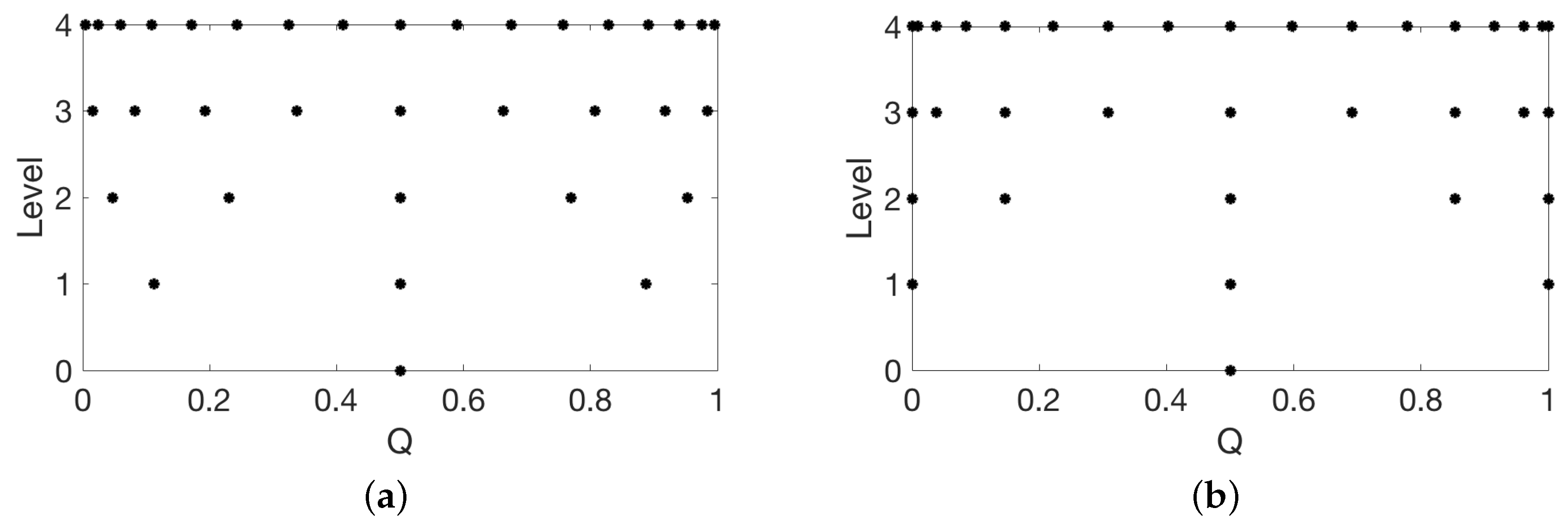
The basis functions, ${\Psi }_j,j=1,\dots ,N$, should be employed in conjunction with a complimentary choice of training points, $q^m,m=1,\dots ,M$, to accurately approximate the ray-tracing model. Training points derived from Gaussian quadrature are often employed, due to their accuracy with relatively few points. However, these points are not nested and hence cannot be re-employed when increasing discretization levels. This is made apparent by Figure 5a,b, in which we plot the Gauss–Legendre and Clenshaw–Curtis points for levels $\ell =0,\dots ,4$, where the number of training points are given by $R\left(\ell \right)=2^{\ell }+1$. We note that each level of Gauss–Legendre points do not overlap with the level above it, whereas the Clenshaw–Curtis points do overlap. This becomes important when attempting to improve a grid without re-evaluating the high-fidelity model at every point on the updated grid. We consider four separate sets of training points and we compare how the surrogate models previously discussed perform when employing each set of points. Whereas there is a whole class of model-based design methods that have been studied for use with various surrogate modeling techniques [37], we consider model-free techniques. Additionally, methods for experimental design could be employed to improve surrogate performance, but we leave this as future work.

The first set of points is Gauss–Legendre (GL), which we use to obtain the surrogate model results discussed in Section 5. The Gauss–Legendre points can be obtained by solving for the roots of the Legendre polynomials. We compile $rRMSE$ results for the surrogate models employing these training points in

Table 4. Comparison of surrogate models relative error using randomly generated training points where Legendre refers to the model constructed via Equation (21) and Legendre Reg. refers to the model constructed via Equation (26).

Points	Legendre	Leg. Reg.	MARS	RBF	GP	NN
GL	$2.13\times {10}^{-1}$	$3.05\times {10}^{-1}$	$4.18\times {10}^{-1}$	$2.08\times {10}^{-1}$	$1.98\times {10}^{-1}$	$2.62\times {10}^{-1}$
Random	$9.39\times {10}^0$	$2.67\times {10}^{-1}$	$3.57\times {10}^{-1}$	$1.12\times {10}^{-1}$	$7.79\times {10}^{-2}$	$2.02\times {10}^{-1}$
CC	$2.26\times {10}^{-1}$	$2.90\times {10}^{-1}$	$4.31\times {10}^{-1}$	$2.21\times {10}^{-1}$	$2.39\times {10}^{-1}$	$2.94\times {10}^{-1}$
LHS	$9.44\times {10}^0$	$3.53\times {10}^{-1}$	$3.60\times {10}^{-1}$	$1.67\times {10}^{-1}$	$1.51\times {10}^{-1}$	$2.26\times {10}^{-1}$

. We also compile in Table 4 the surrogate model $rRMSE$ when randomly selected training points are used. These randomly selected points are drawn from a uniform distribution over $[0,1]$.

Clenshaw–Curtis (CC) quadrature points are specified by the extrema of Chebyshev polynomials, which are typically defined on the interval $[-1,1]$. These points, when mapped to $[0,1]$, are given by

$$q_{\ell }^r=\frac{1}{2}\left[1-cos\frac{(r-1)\pi }{R\left(\ell \right)-1}\right],r=1,\dots ,R\left(\ell \right),$$

(55)

where $R\left(\ell \right)=2^{\ell }+1$. As shown in Figure 5, these points are not equally spaced and cluster around the endpoints of the interval. This effectively avoids producing spurious oscillations, termed the Runge’s phenomenon, when interpolating. Furthermore, we note that these points are nested, so that the training points in level $R\left(\ell \right)$ are also in level $R(\ell +1)$, which is important when more points must be added for increased accuracy of the surrogate model. In practice, it has been shown that, for most functions, Clenshaw–Curtis quadrature performs as well as Gaussian quadrature [38] in most applications.

Latin hypercube points—obtained via latin hypercube sampling (LHS)—were designed to be quasi-random while adequately exploring a multidimensional space [39,40]. For a p dimensional parameter space, each dimension is divided into $\mathcal{M}$ equally probable sections. Then, $\mathcal{M}$ sample points are randomly placed so that each sample is the only point in its axis-aligned hyperplane. This sampling scheme is favorable in high dimensions—e.g., $p\ge 10$—since increased samples are not required for increased dimensions. In addition, these points can be nested, as with Clenshaw–Curtis.

We note that the discrete projection-based Legendre surrogate model employing Gauss–Legendre sampling outperform the same surrogate model employing the other sampling methods. Conversely, the regression-based Legendre, MARS, RBF, Gaussian processes, and neural networks surrogate models favor random sampling of the parameter space. Latin hypercube sampling has been shown to perform about as well as simple random Monte Carlo sampling strategies [39,40]. We attribute the decrease in accuracy seen in a number of the surrogate models employing LHS sampling to the low dimensional parameter space, thus we do not exploit the main strength of Latin hypercube sampling—better accuracy in high dimensional spaces. Additionally, recent work has shown that this is not true when model hyperparameters are unknown and must be estimated from training data observed at the chosen design sites [41].

In

Table 5. Comparison of surrogate model accuracy bounds in $rRMSE$ employing increasingly more Gauss–Legendre training points where Legendre refers to the model constructed via Equation (21) and Legendre Reg. refers to the model constructed via Equation (26).

M	Legendre	Legendre Reg.	MARS	RBF	GP	NN
$9^3$	26.950	0.4244	0.4803	0.3828	0.3804	0.4306
${11}^3$	2.0417	0.4225	0.4341	0.3753	0.3661	0.4713
${13}^3$	0.5061	0.3574	0.4190	0.3220	0.3109	0.5311
${15}^3$	0.3351	0.3390	0.4307	0.2825	0.2738	0.3563
${17}^3$	0.2947	0.3344	0.4025	0.2375	0.2422	0.4164
${19}^3$	0.2427	0.3135	0.3908	0.2397	0.2173	0.3636
${21}^3$	0.2128	0.3048	0.4175	0.2075	0.1975	0.2624

, we tabulate the $rRMSE$ of each of the surrogate models for several choices of the number of tensored Gauss–Legendre points used to train the surrogate models. We note that the Legendre polynomials employing discrete projections do not do well at approximating the physical model for a low number of training points. This likely has to do partly with fewer points being employed for the quadrature rule. The sparsity controlled regression-based Legendre surrogate model does not have this same problem, but the error decreases more slowly than some of the other surrogate models as more training points are employed. The MARS surrogate model does not improve greatly when training points are added. The radial basis function, Gaussian processes, and neural networks surrogate models behave similarly and, as expected, with the $rRMSE$ error bound decreasing as more training points are employed. In Section 5, we employ the Gauss–Legendre points for surrogate model construction, since this choice provides a good comparison of all the surrogate models.

5. Surrogate Performance Results

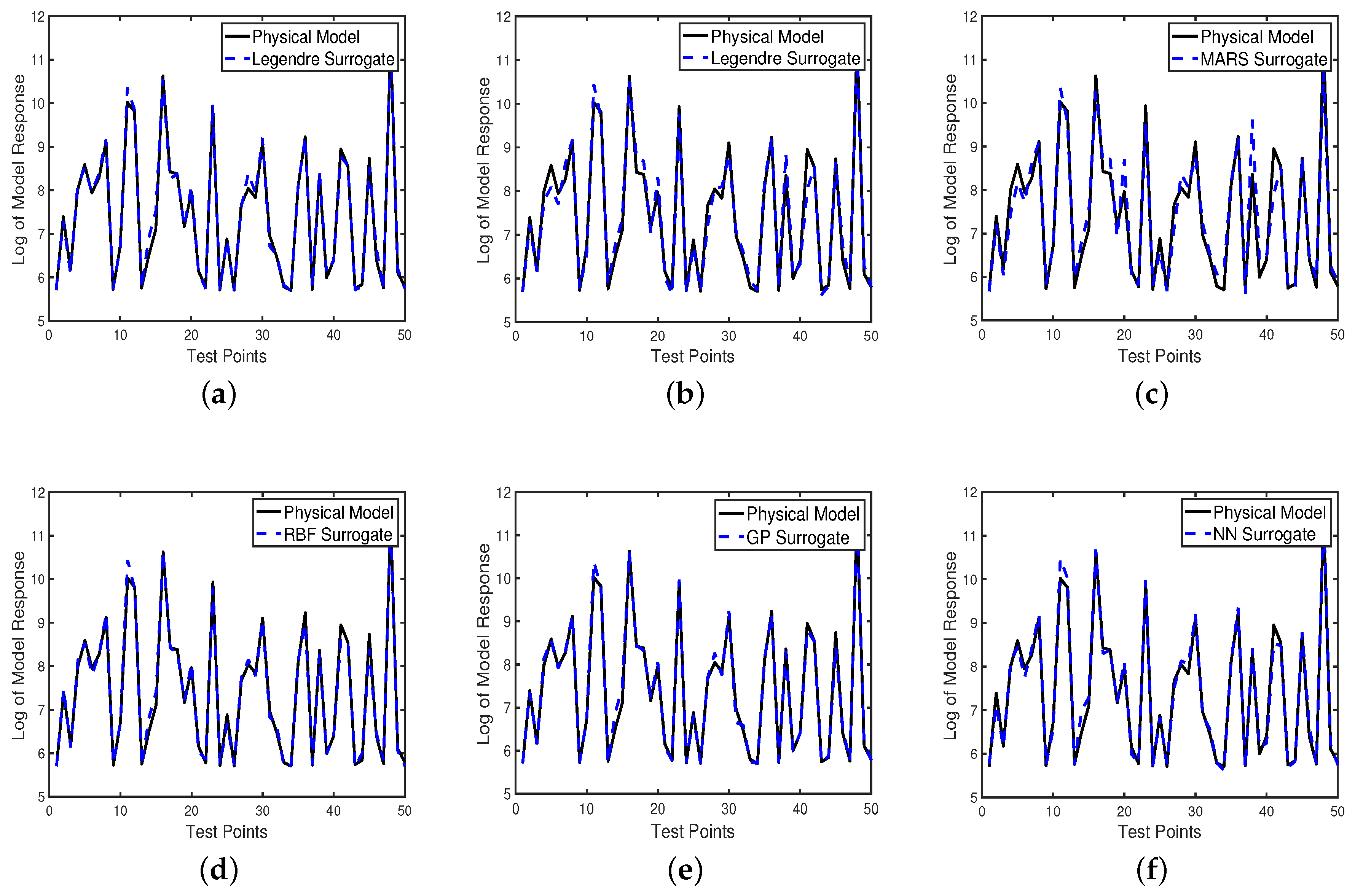
For each of the surrogate models discussed in Section 3, we plot the goodness of fit for the first 50 test points in Figure 6 for detector 1. Note that we construct these surrogate models by employing Gauss–Legendre training points. Figure 6a,b depicts the natural log response of the physical model plotted versus the Legendre polynomial-based surrogate models solved for via discrete projection in Equation (21) and LASSO from Equation (26). Additionally, we plot in Figure 6c–f the natural log of the physical model response versus the response of the surrogate models based on multivariate adaptive regression splines, radial basis functions, Gaussian processes, and neural networks, respectively. We note that each of these surrogate models provides an accurate approximation to the physical model.

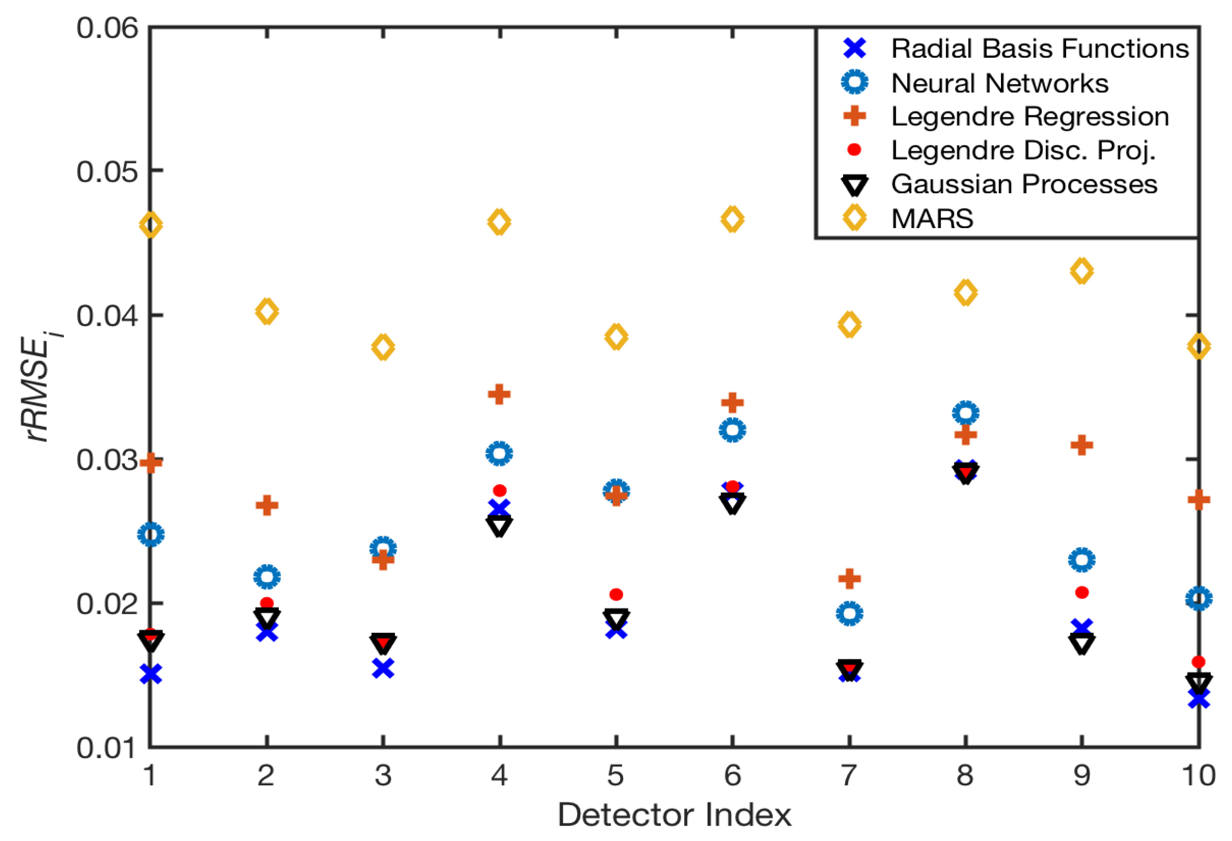
For each of the 10 detector models and for each of the considered surrogate models, we plot the relative root mean squared error ($rRMS{E}_i$) for test points ${\left\{q^s\right\}}_{s=1}^S,s=1,\dots ,S$ in Figure 7. We also compile the total $rRMSE$, defined in Equation (10), for each surrogate model in

Table 6. Comparison of surrogate models using Gauss–Legendre training points where Legendre refers to the model constructed via Equation (21) and Legendre Reg. refers to the model constructed via Equation (26).

Surrogate	rRMSE	Surrogate Computation Time (s)	Surrogate Evaluation Time (s)
Legendre	$2.13\times {10}^{-1}$	33.42	3.86
Legendre Reg.	$3.05\times {10}^{-1}$	50.21	3.95
MARS	$4.18\times {10}^{-1}$	66.43	0.02
RBF	$2.08\times {10}^{-1}$	134.45	0.29
GP	$1.98\times {10}^{-1}$	425.64	2.32
NN	$2.62\times {10}^{-1}$	124.11	0.13

along with the computation and evaluation times of the surrogate models.

Note that, in Figure 6a,b, both methods for computing the Legendre surrogate models produce good approximations to the physical model. However, the results in Table 6 show that the surrogate models computed by employing discrete projection provide better accuracy and efficiency than the surrogate models employing sparsity controlled regression. Whereas the Legendre polynomial-based surrogate models require the least time to compute, they require substantially more time to evaluate due to the large number of basis functions required to accurately approximate the non-smooth behavior of the physical model.

The MARS surrogate models do not perform as well as other surrogate models in terms of accuracy, but outperform many of them in terms of computational speed. This is especially apparent in some of the large deviations of the surrogate model for detector 1 from the test data in Figure 6c as well as by the scale of the $rRMS{E}_i$ in Figure 7. We explain this decrease in accuracy by the fact that MARS is meant to be used on high-dimensional problems. We would expect these surrogate models to be competitive in terms of accuracy with the other surrogate models when approximating a higher dimensional problem. The ability of MARS to accommodate high-dimensional parameter spaces makes it an ideal candidate for problems with a large number of parameters.

The radial basis functions presented in Section 3.3 are isotropic, but the surrogate models based on radial basis functions have low $rRMSE$ in comparison with the other surrogate models, as depicted in Figure 7 and compiled in Table 6. This isotropy is a concern for our non-smooth model when less training points are available, since the model has different responses in each parametric direction, mainly between the $(x,y)$ and I parameters. The Gaussian processes surrogate models are constructed in a way to avoid this problem using anisotropic kernel functions. The Gaussian processes surrogate models are more accurate than the other models, but require a large amount of computation and evaluation time when compared with the other models. However, the combination of the computation and evaluation expenses required by the Gaussian processes surrogate models is still significantly less expensive than the evaluation of the physical model at those same test points.

Radial basis function and neural network surrogate models also provide accurate approximations of the physical model with the trade off of requiring a moderate amount of time to compute the surrogate models. The evaluation time for the RBF and neural networks surrogate models is an order of magnitude smaller than the other surrogate models, excluding the less accurate MARS surrogate models, and substantially smaller than the physical model evaluation time, making them ideal for Bayesian inference and uncertainty quantification.

We used MATLAB’s built-in neural network and Gaussian processes packages to develop these two surrogate models, whereas we constructed the functions required to evaluate the radial basis functions and Legendre functions surrogate models. Additionally, we employed the third-party ARES toolbox [28] for the construction of the MARS surrogate models.

6. Radiation Source Localization

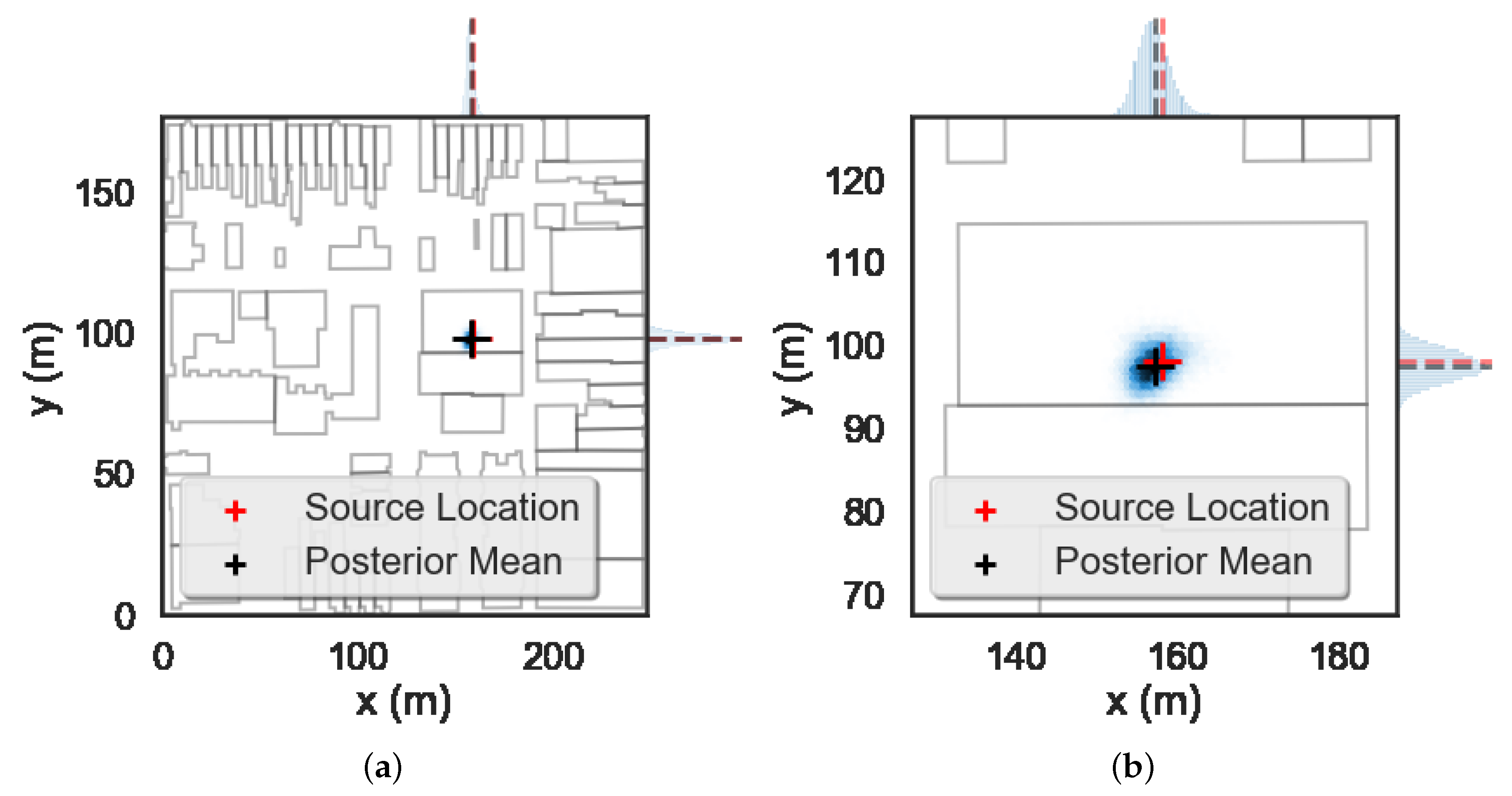
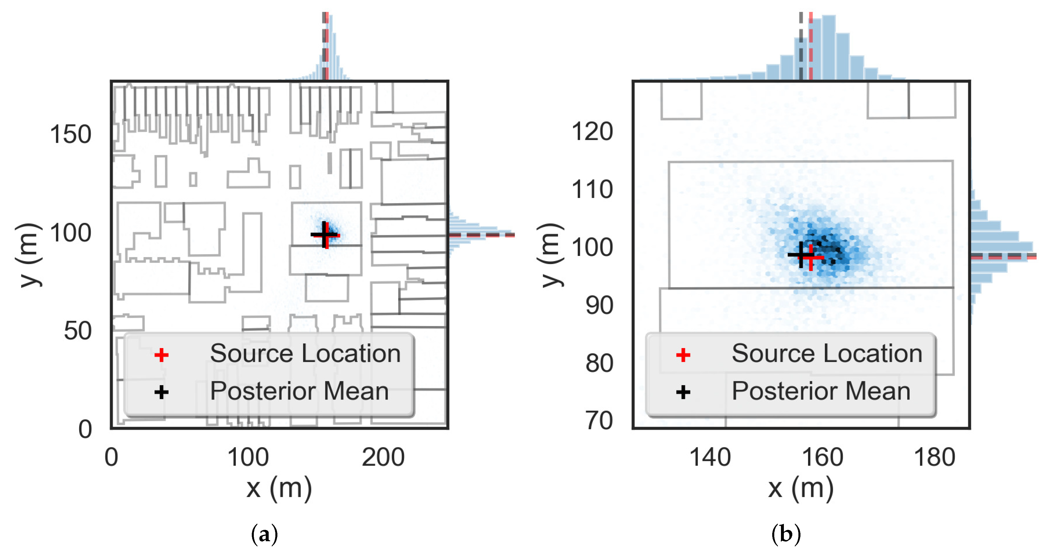
To illustrate the use of these surrogate models for Bayesian inference, we consider the problem of locating a source within the domain depicted in Figure 1 and outlined in Section 2.2. We begin by simulating a $3.22\times {10}^8$ Bq source at the location $(x,y)=(158,98)$ as in Ref. [16]. We then employ the ray-tracing model from Equation (3) to simulate detector responses and DRAM to perform Bayesian inference. A complete description of DRAM and the methodology used for source localization can be found in Ref. [6]. We initialize the MCMC chains in the center of the uniform parameter prior distributions—i.e., an approximately $3.7\times {10}^7$ Bq source in the center of the domain—and we draw ${10}^5$ samples, with the first half discarded as burn-in. Visual inspection of the sample histories indicate that this number of samples is a very conservative choice. We plot the posterior obtained from DRAM in Figure 8 and note that the mode of the posterior is within approximately 1.5 m of the true source location. Additionally, we have captured the true source location within the posterior distribution, which covers approximately a 10 m by 10 m portion of the domain.

Next, we use the same simulated source and employ the surrogate models to generate detector responses to solve the source localization problem with DRAM. We employ the same DRAM setup as with the ray-tracing model and we plot the posteriors in Figure 9. We note that the mode of the posterior is within 2 m of the true source location and that the posteriors are more diffuse than before. The wider posteriors are caused by the model discrepancy errors ${\epsilon }_i^m$ that arise from our smoothing of the ray-tracing model solution. These discrepancies lead to less precise localization results, however we have still accurately localized the source to within a 35 m by 35 m portion of the domain and this amount of precision in the posterior results is sufficient for most applications.

7. Conclusions and Future Work

Our goal is to construct surrogate models that could approximate the non-smooth model solution accurately and inexpensively. We employ surrogate models based on Legendre polynomials, multivariate adaptive regression splines, radial basis functions, Gaussian processes, and neural networks. Table 6 displays the $rRMSE$ of the surrogate models, as well as the computational efficiency of the surrogate models. We see that all of the surrogate models yield a dramatic decrease in the time required to evaluate the model at the 500 test points. The evaluation of the ray-tracing model required nearly 14 min, whereas all the surrogate models required merely seconds for the same evaluation. The relative errors in Table 6 are acceptable for many applications, including for this model. Additionally, we show that the choice of training points is important when choosing a surrogate model and can affect the performance of the surrogate model approximation. We show that the surrogate models investigated here provide sufficiently accurate approximations for use in Bayesian inference when solving the source localization problem.

An area of present and future work is the application of a selection of these surrogate models to approximate high-fidelity 3D radiation transport simulations in a similar urban domain. Whereas these simulations require multiple minutes for a single evaluation with low uncertainty, they incorporate more complex physics and allow for three-dimensional domain construction. However, this computational expense precludes Bayesian inference and motivates the development of surrogate models. An additional area of future work is the use of these surrogate models for optimal detector placement and moving detectors, similar to the work done in Ref. [2,5]. The surrogate models developed here would require being retrained for every new detector location considered for optimal placement, making these surrogate models in their current framework infeasible for use in that problem. However, the surrogate modeling techniques can be reused to approximate, for instance, mutual information to inform optimal surrogate placement.

References

- Brennan, S.; Mielke, A.; Torney, D.; Maccabe, A. Radiation detection with distributed sensor networks. Computer 2004, 37, 57–59. [Google Scholar] [CrossRef] [Green Version]
- Ştefănescu, R.; Schmidt, K.; Hite, J.; Smith, R.C.; Mattingly, J. Hybrid optimization and Bayesian inference techniques for a non-smooth radiation detection model. Int. J. Numer. Methods Eng. 2017, 111, 955–982. [Google Scholar] [CrossRef] [Green Version]
- Chin, J.; Yau, D.K.Y.; Rao, N.S.V.; Yang, Y.; Ma, C.Y.T.; Shankar, M. Accurate localization of low-level radioactive source under noise and measurement errors. In Proceedings of the 6th ACM Conference on Embedded Network Sensor Systems, Raleigh, NC, USA, 5–7 November 2008; pp. 183–196. [Google Scholar]
- Hite, J.M. jasonmhite/gefry2. [online] Github. Available online: Http://github.com/jasonmhite/gefry2 (accessed on 22 June 2018).
- Schmidt, K.; Smith, R.C.; Hite, J.; Mattingly, J.; Azmy, Y.; Rajan, D.; Goldhahn, R. Sequential optimal positioning of mobile sensors using mutual information. Stat. Anal. Data Min. 2019. [Google Scholar] [CrossRef]
- Haario, H.; Laine, M.; Mira, A.; Saksman, E. DRAM: Efficient adaptive MCMC. Stat. Comput. 2006, 16, 339–354. [Google Scholar] [CrossRef]
- Goorley, T.; James, M.; Booth, T.; Brown, F.; Bull, J.; Cox, L.J.; Durkee, J.; Elson, J.; Fensin, M.; Forster, R.A.; et al. Initial MCNP6 release overview. Nucl. Technol. 2012, 180, 298–315. [Google Scholar] [CrossRef]
- Hite, J.M.; Mattingly, J.K.; Schmidt, K.L.; Ştefănescu, R.; Smith, R. Bayesian metropolis methods applied to sensor networks for radiation source localization. In Proceedings of the IEEE International Conference on Multisensor Fusion and Integration for Intelligent Systems, Baden-Baden, Germany, 19–21 September 2016. [Google Scholar]
- Yankov, A. Analysis of Reactor Simulations Using Surrogate Models. Ph.D. Thesis, University of Michigan, Ann Arbor, MI, USA, 2015. [Google Scholar]
- Wang, C.; Duan, Q.; Gong, W.; Ye, A.; Di, Z.; Miao, C. An evaluation of adaptive surrogate modeling based optimization with two benchmark problems. Environ. Model. Softw. 2014, 60, 167–179. [Google Scholar] [CrossRef] [Green Version]
- Bhosekar, A.; Ierapetritou, M. Advances in surrogate based modeling, feasibility analysis, and optimization: A review. Comput. Chem. Eng. 2018, 108, 250–267. [Google Scholar] [CrossRef]
- Forrester, A.; Keane, A. Recent advances in surrogate-based optimization. Prog. Aerosp. Sci. 2009, 45, 50–79. [Google Scholar] [CrossRef]
- Han, Z.-H.; Zhang, K.-S. Surrogate-based optimization. In Real-World Application of Genetic Algorithm; IntechOpen: London, UK, 2012; pp. 343–362. [Google Scholar]
- Ştefănescu, R.; Hite, J.; Cook, J.; Smith, R.C.; Mattingly, J. Surrogate-based robust design for a non-smooth radiation source detection problem. Algorithms 2018, 12, 113. [Google Scholar] [CrossRef] [Green Version]
- Shultis, J.K.; Faw, R.E. Radiation Shielding; American Nuclear Society: La Grange Park, IL, USA, 2000; Chapter 10. [Google Scholar]
- Hite, J.M. Bayesian Parameter Estimation for the Localization of a Radioactive Source in a Heterogeneous Urban Environment. Ph.D. Thesis, North Carolina State University, Raleigh, NC, USA, 2019. [Google Scholar]
- Smith, R.C. Uncertainty Quantification: Theory, Implementation, and Applications; SIAM: Philadelphia, PA, USA, 2014. [Google Scholar]
- Gneiting, T.; Raftery, A.E. Strictly proper scoring rules, prediction, and estimation. J. Am. Stat. Assoc. 2007, 102, 359–378. [Google Scholar] [CrossRef]
- Sullivan, T.J. Introduction to Uncertainty Quantification; Springer: New York, NY, USA, 2015. [Google Scholar]
- Bieglert, L. Large-Scale Inverse Problems and Quantification of Uncertainty; Wiley: Chichester, UK, 2011; pp. 135–136. [Google Scholar]
- Arlot, S.; Celisse, A. A survey of cross-validation procedures for model selection. Stat. Surv. 2010, 4, 40–79. [Google Scholar] [CrossRef]
- Yang, Y. Can the strengths of AIC and BIC be shared? A conflict between model identification and regression estimation. Biometrika 2005, 92, 937–950. [Google Scholar] [CrossRef]
- Friedlander, M.P.; van den Berg, E. Probing the pareto frontier for basis pursuit solutions. SIAM J. Sci. Comput. 2008, 31, 890–912. [Google Scholar]
- Friedman, J.H. Multivariate adaptive regression splines. Ann. Stat. 1991, 19, 1–67. [Google Scholar] [CrossRef]
- Zhang, W.; Goh, A. Multivariate adaptive regression splines for analysis of geotechnical engineering systems. Comput. Geotech. 2013, 48, 82–95. [Google Scholar] [CrossRef]
- Denison, D.G.T.; Mallick, B.K.; Smith, A.F.M. Bayesian MARS. Stat. Comput. 1998, 8, 337–346. [Google Scholar] [CrossRef]
- Green, P.J. Reversible jump Markov chain Monte Carlo computation and Bayesian model determination. Biometrica 1995, 82, 771–832. [Google Scholar] [CrossRef]
- Jekabsons, G. ARESLab: Adaptive Regression Splines Toolbox for Matlab/Octave. Available online: http://www.cs.rtu.lv/jekabsons/ (accessed on 17 May 2018).
- Piret, C. Analytical and Numerical Advances in Radial Basis Functions. Ph.D. Thesis, University of Colorado, Boulder, CO, USA, 2007. [Google Scholar]
- Driscoll, T.A.; Fornberg, B. Interpolation in the limit of increasingly flat radial basis functions. Comput. Math. Appl. 2002, 43, 413–422. [Google Scholar] [CrossRef] [Green Version]
- Choi, I.; Li, B.; Wang, X. Nonparametric estimation of spatial and space-time covariance functions. J. Agric. Biol. Environ. Stat. 2013, 18, 611–630. [Google Scholar] [CrossRef]
- Rasmussen, C.E.; Williams, C.K.I. Gaussian Processes for Machine Learning; MIT Press: Boston, MA, USA, 2006. [Google Scholar]
- Stein, M.L. Interpolation of Spatial Data: Some Theory for Kriging; Springer Series in Statistics; Springer: New York, NY, USA, 1999. [Google Scholar]
- Bastos, L.S.; O’Hagan, A. Diagnostics for Gaussian process emulators. Technometrics 2009, 51, 425–438. [Google Scholar] [CrossRef]
- Marsland, S. Machine Learning: An Algorithmic Perspective; CRC Press: Boca Raton, FL, USA, 2014. [Google Scholar]
- LeCun, Y.; Bengio, Y.; Hinton, G. Deep learning. Nature 2015, 521, 436–444. [Google Scholar] [CrossRef] [PubMed]
- Kaufman, C.G.; Bingham, D.; Habib, S.; Heitmann, K.; Frieman, J.A. Efficient emulators of computer experiments using compactly supported correlation functions, with an application to cosmology. Ann. Appl. Stat. 2011, 5, 2470–2492. [Google Scholar] [CrossRef]
- Trefethen, L. Is Gaussian quadrature better than Clenshaw-Curtis? SIAM Rev. 2008, 50, 67–87. [Google Scholar] [CrossRef]
- Owen, A. Monte Carlo variance of scrambled net quadrature. SIAM J. Numer. Anal. 1997, 34, 1884–1910. [Google Scholar] [CrossRef]
- Stein, M.L. Large sample properties of simulations using latin hypercube sampling. Technometrics 1987, 29, 143–151. [Google Scholar] [CrossRef]
- Zhang, B.; Cole, D.A.; Gramacy, R.B. Distance-distributed design for Gaussian process surrogates. Technometrics 2019, 1–28. [Google Scholar] [CrossRef]
Figure 1.
Satellite image of domain with overlaid model geometry from [2].
Figure 2.
Gaussian process surrogate model response surface versus natural logarithm of the training data for detector 1 observing a source with intensity .
Figure 3.
(a) Sum of squares error and (b) likelihood for Legendre-based surrogate models computed via Equation (21) with maximum polynomial degree . The dashed lines correspond to each of the surrogate models and the solid line is their mean.
Figure 4.
Simple additive MARS example with two knot locations represented by the dashed vertical lines.
Figure 5.
Quadrature points for levels for (a) Gauss–Legendre and (b) Clenshaw–Curtis algorithms.
Figure 6.
Log of detector 1 model responses plotted for the first 50 test points versus the: (a) Legendre surrogate model computed via Equation (21); (b) Legendre surrogate model computed via Equation (26); (c) MARS surrogate model; (d) radial basis functions surrogate model; (e) Gaussian processes surrogate model; and (f) neural networks surrogate model.
Figure 7.
Root mean squared relative error for the 10 surrogate models, corresponding to the 10 detectors, constructed using these methods.
Figure 8.
Posterior density for source location employing the ray-tracing model for Bayesian inference with DRAM. We plot (a) the full domain and (b) the portion of the domain where the posterior is located.
Figure 9.
Posterior density for source location employing the Gaussian processes surrogate model for Bayesian inference with DRAM. We plot (a) the full domain and (b) the portion of the domain where the posterior is located.