Misalignment Fault Prediction of Wind Turbines Based on Combined Forecasting Model

School of Mechanical, Electronic and Control Engineering, Beijing Jiaotong University, Beijing 100044, China
*
Author to whom correspondence should be addressed.
Algorithms 2020, 13(3), 56; https://0-doi-org.brum.beds.ac.uk/10.3390/a13030056
Submission received: 20 January 2020
/
Revised: 27 February 2020
/
Accepted: 27 February 2020
/
Published: 1 March 2020
(This article belongs to the Special Issue Algorithms for Fault Detection and Diagnosis)
Abstract
:Due to the harsh working environment of wind turbines, various types of faults are prone to occur during long-term operation. Misalignment faults between the gearbox and the generator are one of the latent common faults for doubly-fed wind turbines. Compared with other faults like gears and bearings, the prediction research of misalignment faults for wind turbines is relatively few. How to accurately predict its developing trend has always been a difficulty. In this paper, a combined forecasting model is proposed for misalignment fault prediction of wind turbines based on vibration and current signals. In the modelling, the improved Multivariate Grey Model (IMGM) is used to predict the deterministic trend and the Least Squares Support Vector Machine (LSSVM) optimized by quantum genetic algorithm (QGA) is adopted to predict the stochastic trend of the fault index separately, and another LSSVM optimized by QGA is used as a non-linear combiner. Multiple information of time-domain, frequency-domain and time-frequency domain of the wind turbine’s vibration or current signals are extracted as the input vectors of the combined forecasting model and the kurtosis index is regarded as the output. The simulation results show that the proposed combined model has higher prediction accuracy than the single forecasting models.
1. Introduction
The problem of energy shortage and environmental degradation in the world is becoming more and more serious. Wind energy as environmentally friendly and renewable energy has attracted increasing attention [1]. The cumulative installed capacity of global wind power has also steadily increased in recent years [2]. Because wind turbines are often located in remote areas and the working environment is poor, many wind turbines often fail during operation, which greatly reduces their work quality and efficiency and increases maintenance costs [3]. Therefore, how to effectively decrease the risk of fault during the operation of wind turbines has become a difficult problem.
At present, doubly-fed wind turbines (DFWT) have become the main units for large-capacity wind farms [4]. Due to installation errors, deformation after loading or frequent wind speed fluctuations, misalignment between the gearbox and the generator often happens [5]. The misalignment fault of wind turbines belongs to a latent fault [6,7]. This is because when it happens in actual operation, the unit’s operating parameters will not reach their early warning values immediately, but when the fault accumulates to a certain extent, it will seriously damage the unit’s equipment and cause unit shutdown [8]. Therefore, it is necessary to predict the latent trend of misalignment, which can overcome the blindness of handling the fault and avoid more loss of human and material resources.
There are many commonly used signals for mechanical fault prediction, such as vibration signals, current signals, temperature signals, pressure signals, etc. [9,10,11,12,13]. When the equipment fails, the amplitude of the mechanical vibration will increase [14]. Therefore, vibration signals often more quickly and directly reflect the operational status of the equipment. Compared with vibration signals, the current signals can be more easily obtained and are not easily affected by noise. Thus, in this paper, the vibration signal and current signal are regarded as the signal sources to research the misalignment fault of wind turbines.
After the fault signals are obtained, a reasonable and effective prediction method is necessary for accurately predicting the future operational status of the equipment faults. At present, many scholars have studied the prediction techniques for different types of faults [15,16,17]. In order to determine a suitable forecasting model of misalignment fault in wind turbines, the commonly used prediction methods are summarized in Table 1.
For the complex non-linear system, a single forecasting model is not enough to obtain ideal prediction results. Therefore, in order to predict the mechanical fault accurately, the combined forecasting model has attracted more and more attention from scholars. For example, in Ref. [18], the improved Grey Model (GM (1,1)) and the Back Propagation (BP) neural network optimized by Genetic Algorithm (GA) were used as the single forecasting models. The minimum sum of error squares was used as the combination principle to assign appropriate weight coefficients to them. The combined forecasting model had a smaller prediction error. Ref. [19] proposed a calculation method of combined weight coefficients for the unequal weight of error. The combined forecasting model was constructed by Multivariate Grey Model (MGM (1, n)) and Extreme Learning Machine (ELM) neural network. The combined forecasting model was more suitable for predicting the trend of the bearing fault. In Ref. [20], according to the minimum variance principle, Support Vector Machine (SVM) and grey model were combined to make up the shortcomings of single forecasting models. In Ref. [21], SVM was used as the combiner of forecasting models. The Kalman filter, BP neural network and SVM model were used as single forecasting models. The prediction errors of the single forecasting models were larger than that of the combined model. In Ref. [22], the BP neural network was used to determine the weight coefficients of each single forecasting model. The combined forecasting model using GM (1,1,) optimized by Particle Swarm Optimization (PSO) algorithm and SVM optimized by PSO achieved better prediction accuracy for the short-term load of a regional power grid.
Because the wind turbine is a complex non-linear system, when the misalignment fault occurs, the fault signals have both certainty and randomness characteristics [23]. In addition, the misalignment fault samples obtained in this paper are relatively few. It can be indicated from Table 1 that the grey prediction model is suitable for predicting deterministic trends with few samples, while Least Squares Support Vector Machine (LSSVM) is suitable for predicting the non-linear and stochastic trends with few samples and higher speed [24]. Therefore, the grey prediction model and LSSVM are selected to be the prediction methods for the misalignment fault of wind turbines. In the grey prediction models, the MGM (1, n) can use the multivariate characteristic parameters of the fault state as the inputs of the prediction model [25], which can comprehensively reflect the fault state at the previous moment and establish a more accurate prediction model. Therefore, this paper uses MGM (1, n) to predict the misalignment faults of wind turbines. Because MGM (1, n) has the disadvantage of only being suitable for short-term prediction, the rolling prediction method is used to improve MGM (1, n). Compared with the combination of fixed weight coefficient, LSSVM can assign non-linear weight coefficients to the prediction values of single prediction models dynamically, which makes the weight allocated more reasonably. Therefore, in this paper, a combined forecasting model using LSSVM optimized by quantum genetic algorithm (QGA) as a non-linear and variable weight combiner is proposed. The output prediction values of both the LSSVM model optimized by QGA and the improved Multivariate Grey Model (IMGM (1, n)) are input to the non-linear combiner to get the final predicted values. The vibration and current signals from the misalignment fault simulation model of wind turbine demonstrate that the combined forecasting model has higher prediction accuracy than the single ones.
2. Forecasting Method and Application
2.1. Multivariate Grey Model
In 1982, Professor Julong Deng of Huazhong University of Science and Technology proposed the grey system theory, which has good adaptability to small samples and uncertain systems [26]. Because the GM (1,1) model only uses single time series data and it cannot reflect the interaction between multiple variables, some scholars have proposed a MGM (1, n), where n is the number of variables. The MGM (1, n) is not a simple combination of GM (1,1), but a generalization from the univariate GM (1,1) to the multivariate case by solving n differential equations simultaneously [27].
It is assumed that is n sets of time series data, and k is the number of each data set.
The process of establishing a MGM (1, n) prediction model is as follows:
- (1)
- Accumulate the original data to generate a new sequence data :
- (2)
- A system of n-ary first-order ordinary differential equations can be used to express MGM (1, n):Equation (2) can be written in matrix form as:where, , , .
- (3)
- By the method of least squares, the parameter matrices A and B can be estimated. Assume that . The corresponding matrix can be expressed as:where, , , and is the unit matrix.
- (4)
- The predicted values of MGM (1, n) can be obtained.When n = 1, MGM (1, n) model is transformed into GM (1,1) model.
2.2. Improved Multivariate Grey Model
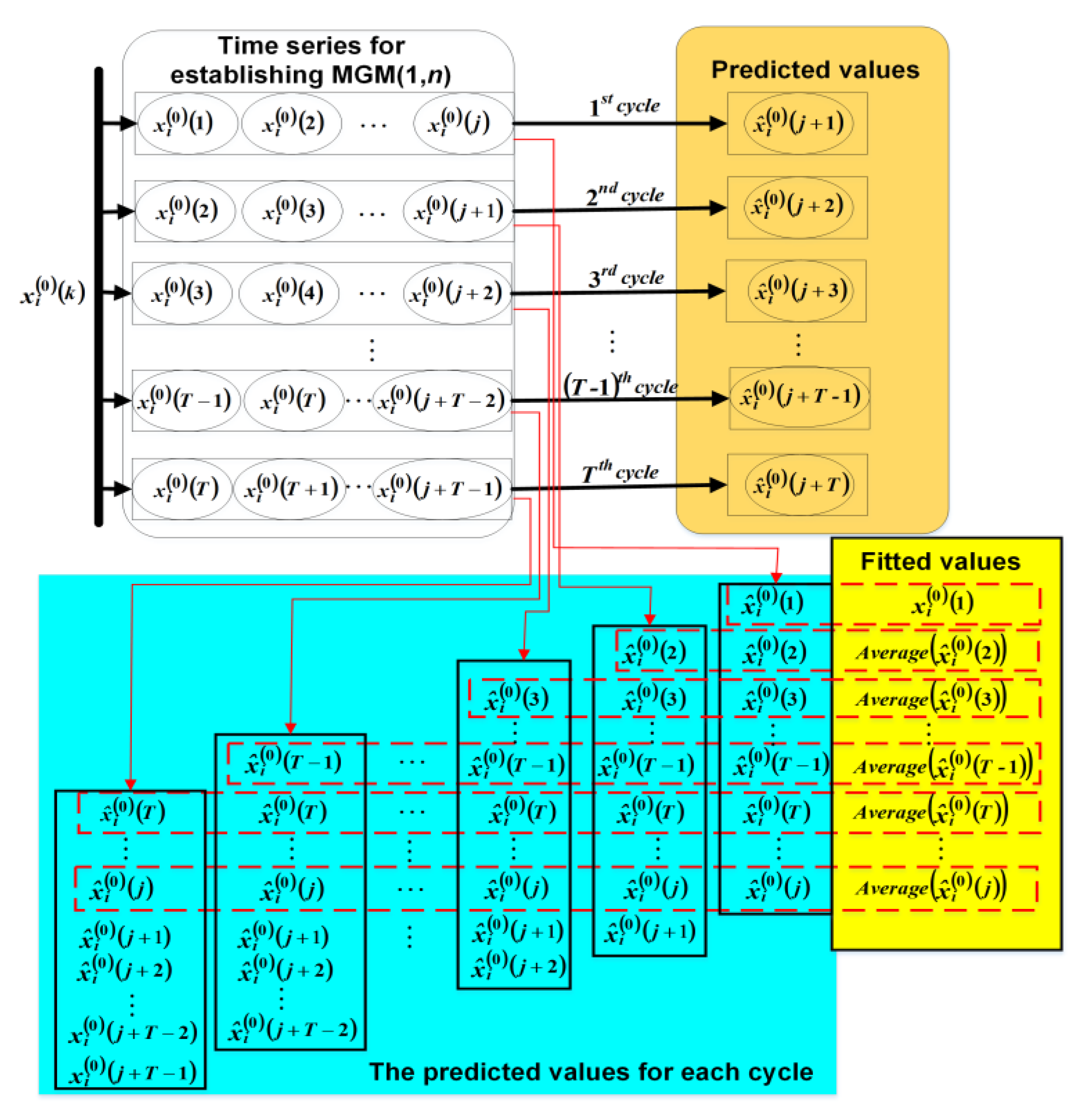
Compared with GM (1, 1), MGM (1, n) has the advantage of considering multiple input features at the same time. However, both the GM (1,1) and MGM (1, n) are not suitable for medium to long-term forecasting. Because the rolling prediction method can make the prediction model achieve medium to long-term forecasting, MGM (1, n) is combined with the rolling prediction method in this paper to get the improved MGM (1, n) prediction model (IMGM (1, n)). The schematic diagram of IMGM (1, n) is shown in Figure 1.
In the IMGM (1, n), based on the establishing process of MGM (1, n), the rolling update of the modelling data is performed by adding the actual value corresponding to the previous step of the current prediction point and removing the first one in the previous modelling data to achieve the dynamic addition of new information. The modelling data is updated every time the model outputs one predicted value.
Assume that is n sets of sequence data. The number of each data set input to the MGM (1, n) is j, which is and . The number of cycles is T and the number of predicted steps for each cycle is one. The predicted process of IMGM (1, n) is as follows:
- As shown in Figure 1, the original data , are used to establish the MGM (1, n). The model outputs one predicted value and j fitted values. The oldest data is removed and the actual data is added to reconstruct the MGM (1, n). The above steps are cycled T times.
- When T cycles are finished, T predicted values after are obtained, and the final j fitted values of each data set output from IMGM (1, n) are the average of the fitted values in the corresponding order for all cycles.
Thus, the IMGM (1, n) is suitable for medium-long prediction. In the application of this paper, the number j of each data set input to the MGM (1, n) model is 45. The number of T is 15. When the 15 cycles are finished, the 45 averages of the fitted values and 15 predicted values will be obtained.
2.3. LSSVM Optimized by Quantum Genetic Algorithm
The Least Squares Support Vector Machine (LSSVM) replaces inequality constraints with equality constraints, regarding the sum of squared errors as experience losses of training set, transforming quadratic programming problems into linear equations [28]. The Radial Basis Function (RBF) is simple to calculate, requiring few parameters to be determined, and with strong generalization ability. The equation of the Radial Basis Function (RBF) is as follows:
where is the kernel width. In this paper, the RBF kernel function is used as the kernel function of LSSVM. The regularization parameter and the parameter of the RBF kernel function have a great influence on the prediction accuracy of LSSVM. If the value of is too large or too small, the generalization ability of the system will be deteriorated. The value of will also affect the performance of the model. Therefore, choosing appropriate parameters can give LSSVM a good prediction effect. In this paper, the QGA is used to realize the adaptive selection of the parameters of LSSVM.
The QGA is an intelligent optimization algorithm combining quantum computing and genetic algorithms, which was proposed by K. H. Han et al. [29]. The probability amplitude representation of qubits is applied to the coding of the chromosome so that a chromosome can express the superposition of multiple states. The operation of quantum revolving gate can update the chromosome, and thus the optimal solution of the goal can be achieved [30]. Compared with GA, QGA has the characteristics of small population size, strong optimization ability, high convergence speed and short calculation time [31].
In GA, the commonly used coding methods for chromosomes are binary coding, real coding and symbol coding. In QGA, chromosomes are encoded using qubits [32].
The state of a qubit can be expressed as:
where, and are complex constants and satisfy . Qubits are used to store and express a gene. The gene can be in a “0” state or a “1” state, or any superposition state of them, which makes QGA have better diversity characteristics than GA. Multi-state genes encoded by qubits are shown in Equation (10).
where, is the chromosome of the generation; and contain the quantization information of the gene. k is the number of qubits of each gene and m is the number of chromosome genes.
For QGA, the quantum revolving gate in quantum theory is used to achieve population update. The operations of selection, crossover and mutation of GA are not adopted. The matrix of quantum revolving gate is expressed as Eequation (11):
The update process is as follows:
where, is the qubit of the chromosome. is the new qubit after the update. is the rotation angle and it is determined according to a previously designed adjustment strategy [33].
Before using QGA to optimize the parameters of LSSVM, the fitness function needs to be defined first. In this paper, the Root Mean Square Error (RMSE) is used as the objective function. The calculation formula of RMSE is shown in Equation (13):
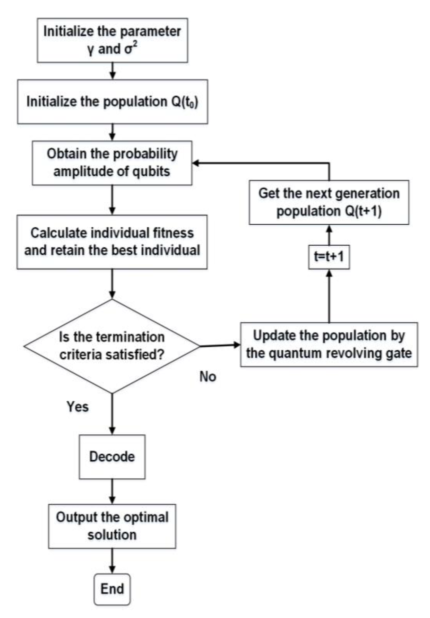
where, is the actual value of the sample; is the predicted value of the sample; , , . The idea of parameter optimization of LSSVM model is to search for a set of parameters through the iterative of QGA to minimize the objective function. The flow chart of QGA is shown in Figure 2. In this paper, the searching range of the regularization parameter is set to [0.1, 100], the searching range of the parameter of kernel function is [0.01, 100], the maximum number of iterations is 200 and the population size is 20, and the coded length of the quantum chromosome is 20.
2.4. Combined Prediction
The combined prediction was first proposed by Bates. J. M and Granger. C. W. J. The combined forecasting model is constructed by assigning different weights to the prediction values of single forecasting models [34]. The classification of combined prediction can be divided into the following two types:
- According to the functional relationship between the combined and the single forecasting models, the combined forecasting model can be divided into linear and non-linear combination prediction [35].
- According to the weight coefficients of the single models, the combined forecasting model can be divided into fixed weight and variable weight combination prediction [36].
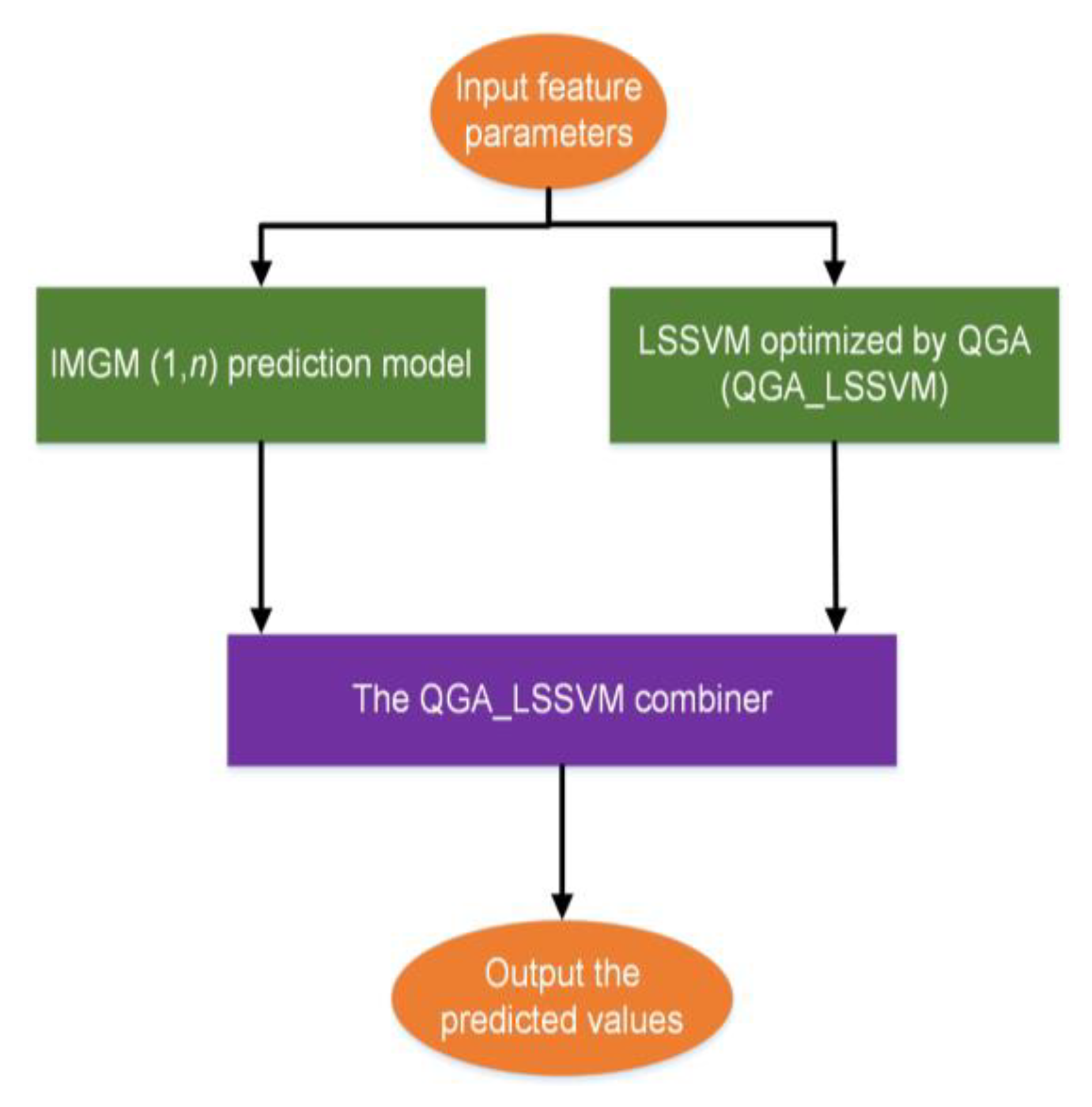
The linear combination prediction has relatively large errors and has great limitations, while the fixed weight combination prediction cannot dynamically adjust the combination weight, therefore it is necessary to use a non-linear and variable weight combined forecasting model. For example, neural networks and SVM are non-linear combiners, and these two combination methods can realize non-linear and variable weight combination of the single forecasting models. However, neural networks are not suitable for processing few samples data. There will be overfitting problems and the prediction accuracy is not satisfactory [37]. SVM or LSSVM has obvious advantages in solving few samples, non-linear and high-dimensional problems [38]. Therefore, LSSVM optimized by QGA is adopted in this paper as a non-linear and variable weight combiner. The flow chart of the proposed combined prediction is shown in Figure 3.
2.5. Evaluation Criteria for Forecasting Models
2.5.1. Accuracy Test of Grey Prediction Model
After the grey prediction model is established, the model can be used to predict effectively only after the accuracy test is qualified. The posteriori error test is adopted in this paper. The equations of posteriori error test are as follows.
The posteriori error ratio C:
where, is the standard deviation of the original sequence and is the standard deviation of the residual sequence.
The small error probability P:
where, is the residual error and is the residual average.
The smaller the value of C and the greater the value of P, the higher the grade of the grey prediction model. Generally, the accuracy grade of the grey prediction model can be divided into four levels which are shown in Table 2.
2.5.2. Forecasting Evaluation Index
In order to compare the prediction effects of the combined model and the single ones, the following 3 indexes are calculated.
Assume that is the actual value of the data, is the predicted value, and is the average of the actual value.
Root Mean Square Error (RMSE):
The closer the RMSE is to zero, the smaller the prediction error and vice versa.
Mean Absolute Error (MAE):
The closer the MAE is to zero, the smaller the prediction error and vice versa.
Coefficient of determination (R2):
The larger the R2 is and the closer it is to 1, the better the fitting effect of the prediction model and vice versa [39].
3. Signal Acquisition and Feature Extraction
3.1. Signal Acquisition
A 1.5 MW wind turbine is taken as the research object in this paper. The three-dimensional model of the 1.5 MW wind turbine drive system is established by Solidworks, and then it is imported into ADAMS for dynamic simulation. In the dynamic simulation model, parallel misalignment, angular misalignment and comprehensive misalignment are simulated. The acceleration signal of the high-speed output of the gearbox is used as the vibration signal (details in literature [40]). In MATLAB, the wind turbine and its control system are established to obtain the stator current for misalignment faults (details in literature [41]). The simulation model of the wind turbine is in the Maximum Power Points Tracking (MPPT) stage, in which the input speed is 81.3°/s, and the vibration signal and stator current signal are obtained under parallel misalignment fault for researching.
3.2. Feature Extraction
3.2.1. Time-Domain Feature Parameters
Time-domain analysis is used to directly obtain the time-domain statistical parameters of fault signals in the time domain. It can simply and intuitively represent the changes of the fault signals. The time-domain feature parameters include dimensional parameters and dimensionless parameters. Assume that the signal obtained is a discrete sequence with finite length, where N represents the number of data points of each sample. Three commonly used time-domain feature parameters are used in the paper. The equations are as follows.
Root Mean Square (RMS):
The RMS represents the average energy measure of the signal and is very stable [42].
Kurtosis:
The kurtosis is highly sensitive to early faults and impact signals, but its stability is poor [43,44].
Kurtosis index:
The kurtosis index is very sensitive to the impact of vibration signals [45].
3.2.2. Frequency-Domain Feature Parameters
Time-domain analysis can only briefly and roughly represent the fault of the device, but it cannot find the inherent cause of the fault. Frequency-domain analysis can transform the signal from the time-domain to the frequency-domain through Fourier transform. Different frequency components are clearly displayed to find the fault frequency. Assume that is a finite-length discrete time series and the sampling frequency is . The calculation equation of commonly used frequency-domain feature parameters are as follows.
Mean Square Frequency (MSF):
Centroid Frequency (FC):
Variance Frequency (VF):
where is the power spectrum of the signal. , . is the discretized angular frequency.
3.2.3. Time-Frequency Domain Feature Parameters
The Empirical Mode Decomposition (EMD) improved by mirror extension is used to process the vibration signal [46]. The advantage of this method is the suppression of endpoint effects. The energy entropy, which is suitable for non-stationary and non-linear complex signals [47], is extracted from the processed vibration signal.
The equation of energy entropy is as follows:
where, ; is the amplitude of each discrete point; is the energy of each Intrinsic Mode Function (IMF) component, and is the total energy of the signal. After vibration signals at different times being decomposed by IEMD, the number of IMF may be different. Therefore, the correlation coefficient method is used to determine the effective number of IMF components. Assume that the non-stationary signal is decomposed into a finite number of uncorrelated components by IEMD. The correlation coefficient between each IMF and the original signal can be calculated as:
where, and . The larger the correlation coefficient, the greater the degree of correlation and vice versa. When , it usually indicates that the IMF has a good correlation with the original signal [49].
The stator current signal obtained from the simulation model is decomposed into 4 layers by the Dual-tree Complex Wavelet Transform (DTCWT) [50]. The obtained 5 sub-band signals are reconstructed and the sample entropy is calculated. Sample entropy can obtain better and more stable results with less data and has stronger robustness [51]. For finite sequences , the equation for the sample entropy is as follows:
where, m is the number of dimensions of the constructed vector, r is a given threshold, and is the average of the maximum distance between two m-dimensional vectors.
3.3. Feature Vectors and Normalization
The input speed of the dynamic simulation model of the wind turbine drive system is set to be 81.3°/s. Afterwards, 60 segments of vibration and current signals of parallel misalignment faults are collected. The time-domain, frequency-domain and time-frequency domain feature parameters of each signal segment are extracted to construct feature vectors. After extracting the time-frequency domain feature parameters of the vibration signal, the correlation coefficients of the first three IMFs of the vibration signal decomposed by IEMD are all greater than 0.1. Therefore, the first three IMFs are selected as effective components in this paper. The feature parameters of vibration and current signal are listed in Table 3 and Table 4.
The fault feature parameters have different orders of magnitude. In order to facilitate the processing of data and ensure that the program runs faster when it converges, the Mapminmax function is used to normalize the time-domain, frequency-domain and time-frequency domain feature parameters in this paper. The equation of Mapminmax function is as follows:
where, is an unnormalized matrix, is a minimum value of the normalization interval, and is a maximum value of the normalization interval. The feature parameters are normalized to the range [0, 1] in this paper.
4. Fault Prediction Results and Discussion
4.1. Fault Prediction Results and Discussion of Vibration Signals
4.1.1. The Results of IMGM (1, n)
The MGM (1, n) is suitable for the prediction of few samples and the required number of modelling is usually between 5 and 60 [52,53,54]. Therefore, the collected 60 vibration signal samples are divided into the first 45 samples and the last 15 samples according to the ratio of 3:1. The first 45 samples are used to construct an IMGM (1, n) prediction model. The indexes of the posteriori error test calculated from the fitted values are listed in Table 5.
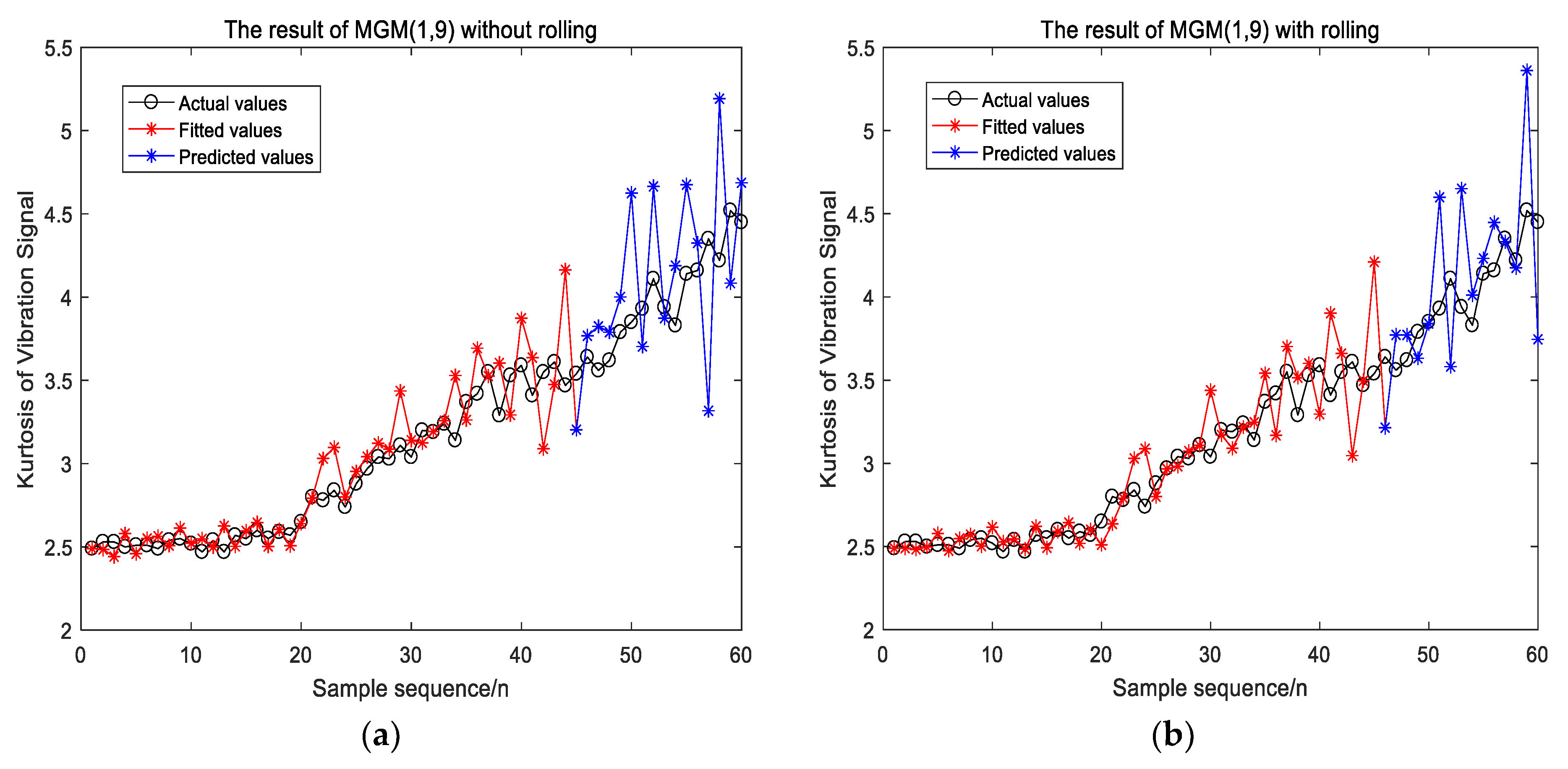
It can be shown from Table 5 that the models of MGM (1,9) and IMGM (1,9) belong to the qualification grade, so they can be used for prediction. Because the C value of IMGM (1,9) is smaller and the P value of IMGM (1,9) is larger, IMGM (1,9) is more suitable for predicting the kurtosis of vibration signals than MGM (1,9). Figure 4 shows the prediction results of MGM (1,9) and IMGM (1,9) of vibration signals.
In Figure 4, the predicted and fitted values of MGM (1,9) and IMGM (1,9) both fluctuated up and down around their actual values. The forecasting evaluation indexes of IMGM (1,9) and MGM (1,9) are listed in Table 6. For the fitted values, the RMSE and R2 of IMGM (1,9) is nearly the same to that of MGM (1,9), while the MAE of IMGM (1,9) is better than that of MGM (1,9). For the predicted values, the RMSE, MAE, and running time of the IMGM (1,9) are smaller than those of MGM (1,9). The R2 of IMGM (1,9) is larger than that of MGM (1,9). Therefore, IMGM (1,9) improves the prediction accuracy of MGM (1,9) for misalignment fault vibration signal of wind turbine. This is because when predicting the last 15 points, the data used to establish the MGM (1,9) model has always been the first 45 points, and the data has not been updated with the increase prediction steps. However, the modelling data of IMGM (1,9) is updated by adding the actual value corresponding to the previous step of the current prediction point. The modelling data is updated every time the model output one predicted value. Hence, the IMGM (1,9) can be one of the single prediction models input to the combined forecasting model for vibration signal.
4.1.2. The Results of LSSVM Optimized by QGA
The LSSVM optimized by QGA (QGA_LSSVM) is also adopted to predict the kurtosis of misalignment fault. The same first 45 samples are used to train the LSSVM model. The other 15 samples are used as the testing set. The results are compared with the LSSVM optimized by GA (GA_LSSVM) and the LSSVM optimized by Grid Search (Grid Search_LSSVM). The parameters obtained by the three prediction models are listed in Table 7.
The three forecasting models are established based on the optimized parameters in Table 7. The corresponding forecasting evaluation indexes are listed in Table 8.
In Table 8, for the training set, the indexes of Grid Search_LSSVM show that it has smaller prediction errors of training set than GA_LSSVM and QGA_LSSVM. For the testing set, the RMSE and MAE of QGA_LSSVM are smaller than those of GA_LSSVM and Grid Search_LSSVM. The R2 of QGA_LSSVM is the largest and its running time is the shortest. Therefore, compared with the results of Grid Search_LSSVM and GA_LSSVM, QGA_LSSVM has the best prediction accuracy and the shortest running time, so it can be one of the single forecasting models input to the combined forecasting model for vibration signal.
4.1.3. The Results of the Combined Forecasting Model
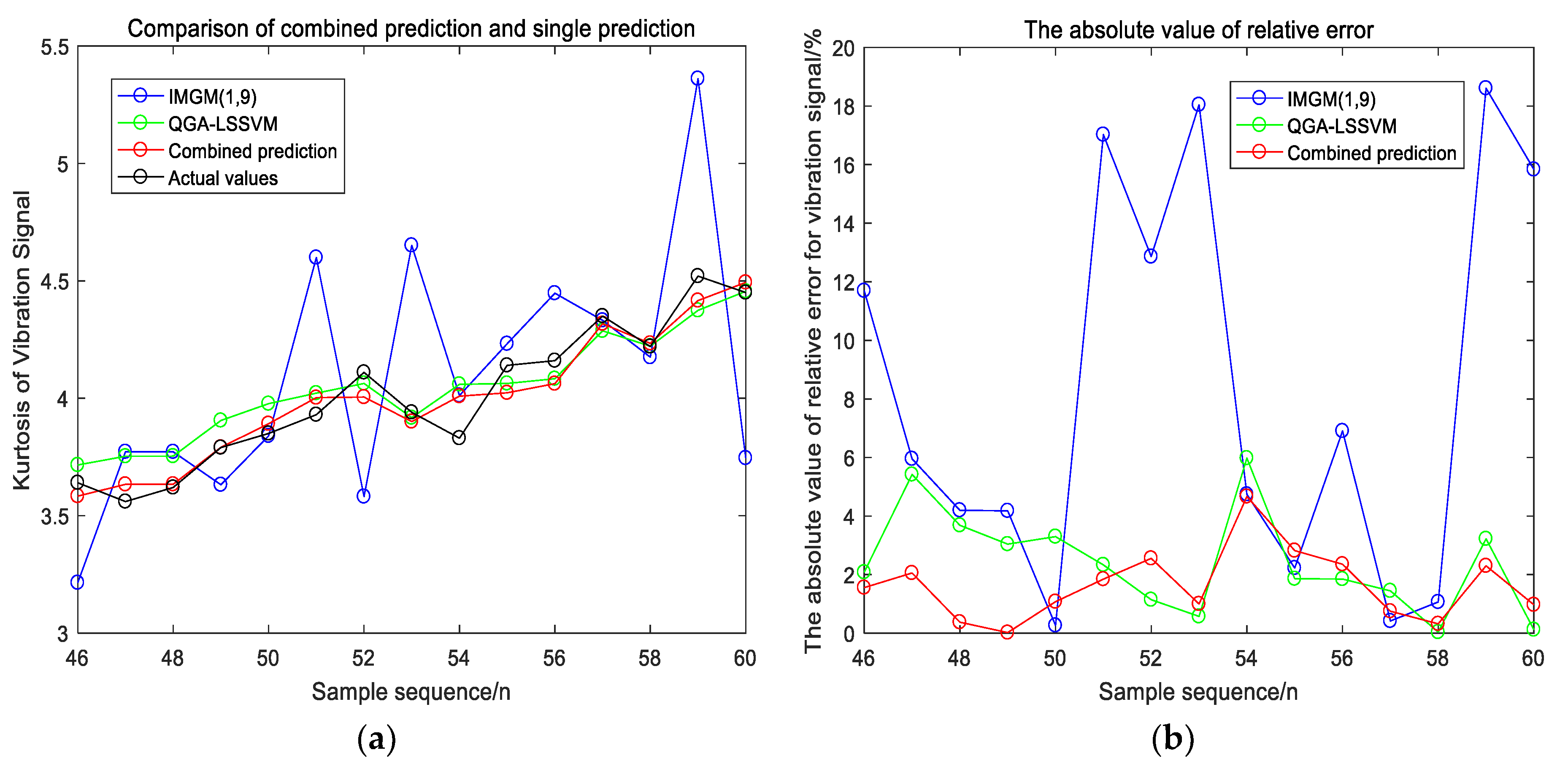
In this paper, the prediction results of IMGM (1,9) and QGA_LSSVM are used as the inputs of QGA_LSSVM combiner and the actual kurtosis values of the vibration signal are used as the output. The comparison of predicted results between the single forecasting models and combined model are shown in Figure 5.
In Figure 5a, the fluctuation range of IMGM (1,9) around the actual value is the largest. The prediction results of QGA_LSSVM and the combined forecasting model are closer to the actual value. Figure 5b shows that the absolute value of relative error of IMGM (1,9) is significantly large. From the 46th predicted points to the 51th predicted points, the absolute value of relative error of the combined forecasting model is less than that of QGA_LSSVM. After the 53th predicted point, they have similar absolute value of relative error. Therefore, the combined forecasting model has a smaller absolute value of relative error than the two single forecasting models. It can also be shown from Table 9 that, for the training test, the forecasting evaluation indexes of the combined forecasting model are near to those of QGA_LSSVM and better than those of IMGM (1,9); but for the testing set, the indexes of the combined forecasting model are the best in Table 9. Thus, compared with the single forecasting models, the combined forecasting model improves the prediction accuracy and reduces the running time for the vibration signal.
For vibration signal, the optimal parameters of the combiner are .
4.2. Fault Prediction Results and Discussion of Current Signal
4.2.1. The Results of IMGM (1, n)
The collected 60 current signal samples are also divided into the first 45 samples and the last 15 samples according to the ratio of 3:1. The first 45 samples are also used to construct an IMGM (1, n) prediction model. Eleven feature parameters of the current signal are used as inputs and the kurtosis is used as output. The indexes of the posteriori error test of current signal are listed in Table 10.
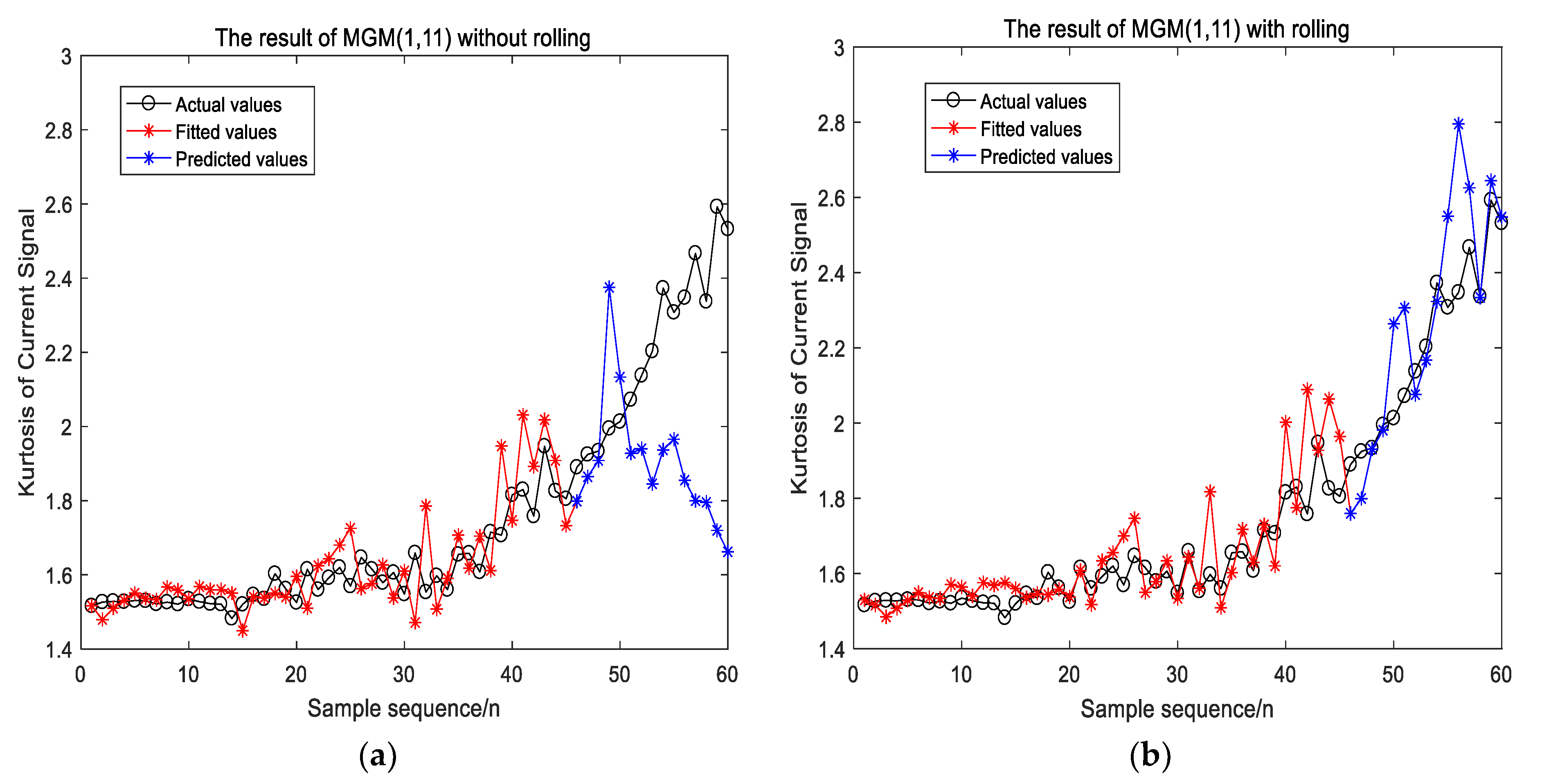
In Table 10, MGM (1,11) is barely qualified grade and IMGM (1,11) belongs to the qualified grade. Therefore, IMGM (1,11) is more suitable for predicting the kurtosis of the current signal than MGM (1,11). The prediction results of MGM (1,11) and IMGM (1,11) of the current signal are shown in Figure 6.
By comparing the prediction results in Figure 6a,b, the predicted fluctuation range of IMGM (1,11) is obviously smaller than that of MGM (1,11). It is because when predicting the last 15 points, the data used to establish the MGM (1,11) has always been the first 45 points, and the data has not been updated with the increase prediction steps. However, the modelling data of IMGM (1,11) is updated by adding the actual value corresponding to the previous step of the current prediction point. The modelling data is updated every time the model outputs one predicted value. Hence, when predicting the kurtosis of a current signal with a large rising slope, the IMGM (1,11) has significantly better prediction accuracy than that of MGM (1,11). The forecasting evaluation indexes of IMGM (1,11) and MGM (1,11) are listed in Table 11. For the fitted values, the RMSE of IMGM (1,11) is nearly the same to that of MGM (1,11), while the MAE and R2 of IMGM (1,11) in the table is better than those of MGM (1,11). For the predicted values, the RMSE, MAE and running time of the IMGM (1,11) are smaller than those of MGM (1,11). The R2 of IMGM (1,11) is much larger than that of MGM (1,11). Therefore, compared with MGM (1,11), IMGM (1,11) improves the prediction accuracy and stability of the current signal, and it can be one of the single prediction models input to the combined forecasting model for current signal.
4.2.2. The Results of LSSVM Optimized by QGA
For the current signal, Grid Search_LSSVM, GA_LSSVM and QGA_LSSVM are also used for prediction. The same first 45 current samples are also used to train the LSSVM. The other 15 samples are also used as the testing set. The optimized parameters obtained by the three prediction models are listed in Table 12.
The three forecasting models are established based on the optimized parameters in Table 12. The corresponding forecasting evaluation indexes are listed in Table 13.
For the training set, the Grid Search_LSSVM has smaller errors than GA_LSSVM and QGA_LSSVM. For the testing set, all of forecasting evaluation indexes of QGA_LSSVM are better than those of GA_LSSVM and Grid Search_LSSVM in Table 13. Thus, QGA_LSSVM has a good prediction effect not only for the vibration signal but also for the current signal, and QGA_LSSVM can be one of the single forecasting models input to the combined forecasting model for the current signal.
4.2.3. The Results of the Combined Forecasting Model
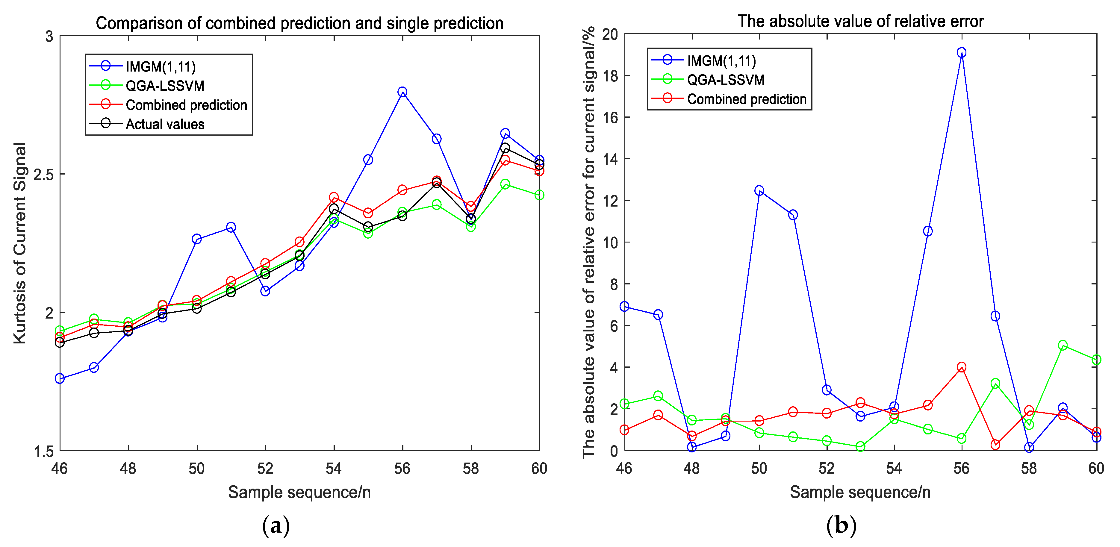
The prediction results of IMGM (1,11) and QGA_LSSVM are used as the inputs of the QGA_LSSVM combiner, and the actual kurtosis values of the current signal are used as the output. The predicted results are shown in Figure 7.
Figure 7a indicates that, compared with IMGM (1,11), the prediction results of QGA_LSSVM and the combined forecasting model are closer to the actual values. In Figure 7b, the absolute value of relative error of QGA_LSSVM and combined forecasting model is within 6%. The absolute value of relative error of IMGM (1,11) is much larger than those of other models. In Table 14, for the training set, the forecasting evaluation indexes of the combined forecasting model are near to those of QGA_LSSVM and better than those of IMGM (1,11), but for the testing set, the indexes of the combined forecasting model are the best. Therefore, it is proved by current signals that the combined forecasting model has a higher prediction accuracy with less running time.
For the current signal, the optimal parameters of the combiner are .
5. Conclusions
To improve the prediction accuracy of single forecasting models, this paper proposes a combined forecasting model using LSSVM optimized by QGA as a combiner to predict the misalignment fault of wind turbines based on vibration and current signals. The specific method is to extract the time-domain, frequency-domain and time-frequency domain feature parameters from the signals at first. After being normalized, the extracted features are used to predict by IMGM (1, n) and QGA_LSSVM separately and the predicted values are then regarded as the inputs of the combiner, which dynamically assigned non-linear weight coefficients to them. The simulation results indicate that the prediction accuracy of the combined prediction model is higher than those of single models and the running time is shortened. This new model is suitable for fault prediction with deterministic and random trends. In future research, the kurtosis predicted by the proposed model will be combined with the kurtosis threshold to achieve early warning of wind turbine misalignment faults.
Author Contributions
Y.X. and Z.H. contributed to paper writing and the whole revision process. All authors have read and agreed to the published version of the manuscript.
Funding
This research was funded by the National Natural Science Foundation of China (51577008).
Acknowledgments
The authors are grateful to the anonymous reviewers for their constructive comments on the previous version of the paper.
Conflicts of Interest
The authors declare no conflicts of interest.
References
- Bandoc, G.; Shop, R.; Patriche, C.; Deprived, M. Spatial assessment of wind power potential at global scale. A geographical approach. J. Clean. Prod. 2018, 200, 1065–1086. [Google Scholar] [CrossRef]
- Arshad, M.; O’Kelly, B. Global status of wind power generation: Theory, practice, and challenges. Int. J. Green Energy 2019, 16, 1073–1090. [Google Scholar] [CrossRef]
- Koltsidopoulos, P.A.; Thies, P.R.; Dawood, T. Offshore wind turbine fault alarm prediction. Wind Energy 2019, 22, 1779–1788. [Google Scholar] [CrossRef]
- Liu, Z.; Zhang, L. A review of failure modes, condition monitoring and fault diagnosis methods for large-scale wind turbine bearings. Meas. J. Int. Meas. Confed. 2020, 149, 107002. [Google Scholar] [CrossRef]
- Xiao, Y.; Wang, Y.; Mu, H.; Kang, N. Research on Misalignment Fault Isolation of Wind Turbines Based on the Mixed-Domain Features. Algorithms 2017, 10, 67. [Google Scholar] [CrossRef] [Green Version]
- Liao, M.; Liang, Y.; Wang, S.; Wang, Y. Misalignment in Drive Train of Wind Turbines. J. Mech. Sci. Technol. 2011, 30, 173–180. [Google Scholar]
- Tonks, O.; Wang, Q. The detection of wind turbine shaft misalignment using temperature monitoring. CIRP J. Manuf. Sci. Technol. 2017, 17, 71–79. [Google Scholar] [CrossRef] [Green Version]
- Kusiak, A.; Li, W. The prediction and diagnosis of wind turbine faults. Renew. Energy 2011, 36, 16–23. [Google Scholar] [CrossRef]
- Liu, Y.; Qiao, N.; Zhao, C.; Zhuang, J. Vibration signal prediction of gearbox in high-speed train based on monitoring data. IEEE Access 2018, 6, 50709–50719. [Google Scholar] [CrossRef]
- Kavousi-Fard, A.; Su, W. A Combined Prognostic Model Based on Machine Learning for Tidal Current Prediction. IEEE Trans. Geosci. Remote Sens. 2017, 55, 3108–3114. [Google Scholar] [CrossRef]
- Liu, Z.; Zhang, L.; Carrasco, J. Vibration analysis for large-scale wind turbine blade bearing fault detection with an empirical wavelet thresholding method. Renew. Energy 2020, 146, 99–110. [Google Scholar] [CrossRef]
- Zhao, H.; Zhang, X.; Guo, W. Early fault prediction of wind turbine drive train system. In Proceedings of the 6th IASTED Asian Conference on Power and Energy Systems, Phuket, Thailand, 10–12 April 2013. [Google Scholar]
- Yang, Y.; Bai, Y.; Li, C.; Yang, Y. Application Research of ARIMA Model in Wind Turbine Gearbox Fault Trend Prediction. In Proceedings of the 2018 International Conference on Sensing, Diagnostics, Prognostics, and Control (SDPC), Xi’an, China, 15–17 August 2018. [Google Scholar]
- Amarnath, M.; Shrinidhi, R.; Ramachandra, A.; Kandagal, S.B. Prediction of defects in antifriction bearings using vibration signal analysis. J. Inst. Eng. Mech. Eng. Div. 2004, 85, 88–92. [Google Scholar]
- Wu, G.; Liang, P.; Long, X. Forecasting of Vibration Fault Series of Stream Turbine Rotor Based on ARMA. J. South China Univ. Technol. 2005, 33, 67–73. [Google Scholar]
- Shi, M.; Jiang, L.; Fu, Y. Study on Prediction Methods for the Fault State of Rotating Machinery Based on Dynamic Grey Model and Metabolism Grey Model. Wirel. Pers. Commun. 2018, 102, 3615–3627. [Google Scholar] [CrossRef]
- Yu, H.; Li, H.; Tian, Z.; Wang, Y. Rolling bearing fault trend prediction based on composite weighted KELM. Int. J. Acoust. Vibr. 2018, 23, 217–225. [Google Scholar] [CrossRef]
- Zhang, K. Research on Hub Bearing Fault Prediction Based on Combination Model; Henan University of Science and Technology: Henan, China, 2017; Available online: http://cdmd.cnki.com.cn/Article/CDMD-10464-1017829413.htm (accessed on 10 January 2019).
- Xu, Y. Rolling element bearing Fault prediction based on Grey Sequential Extreme learning machine. Comput. Meas. Control 2017, 25, 63–65. [Google Scholar]
- Wang, P.; Li, Y.; Zong, X. The new forecasting method of combination based on SVM and grey. J. Hebei Acad. Sci. 2008, 25, 5–7. [Google Scholar]
- Yan, H.; Lu, J.; Qin, Q.; Zhang, Y. A Nonlinear Combined Model for Wind Power Forecasting Based on Multi—attribute Decision—making and Support Vector Machine. Autom. Elec. Power Syst. 2013, 37, 29–34. [Google Scholar]
- Zhang, A. Research on Combination Forecasting Method of Regional Power Grid under Short-Term Load; North China Electric Power University: Baoding, China, 2008; Available online: http://www.wanfangdata.com.cn/details/detail.do?_type=degree&id=Y1455060 (accessed on 10 January 2019).
- Kong, X.; Liu, X.; Lee, K.Y. Data-driven modelling of a doubly fed induction generator wind turbine system based on neural networks. IET Renew. Power Gener. 2014, 8, 849–857. [Google Scholar] [CrossRef]
- Wang, H.; Hu, D. Comparison of SVM and LS-SVM for regression. In Proceedings of the 2005 International Conference on Neural Networks and Brain Proceedings, Beijing, China, 13–15 October 2005. [Google Scholar]
- Zhao, M.; Gao, H.; Xu, M.; Guo, Z.; Qiao, H.; Wu, X.; Huang, B. Application of multi-variable grey model for ball screw remaining life prediction. Comput. Integr. Manuf. Syst. 2011, 17, 846–851. [Google Scholar]
- Huang, D.; Huang, L. Present Situation and Development Tendency of Grey System Theory in Fault Forecast Application. J. Gun Launch Control 2009, 24, 88–92. [Google Scholar]
- Lou, Y.; Zhang, Q.; Liu, G.; Fan, Q. Application of grey multi-variable forecasting model in predicting urban water consumption. Water Resour. Prot. 2005, 21, 11–13. [Google Scholar]
- Liu, S.; Xu, L.; Li, D.; Zeng, L. Dissolved oxygen prediction model of eriocheir sinensis culture based on least squares support vector regression optimized by ant colony algorithm. Trans. Chin. Soc. Agric. Eng. 2012, 28, 167–175. [Google Scholar]
- Han, K.H.; Kim, J.H. Genetic quantum algorithm and its application to combinatorial optimization problem. In Proceedings of the 2000 Congress on Evolutionary Computation, La Jolla, CA, USA, 16–19 July 2000; IEEE Computer Society. [Google Scholar]
- Zhang, X.; Sui, G.; Zheng, R.; Li, Z.; Yang, G. An Improved Quantum Genetic Algorithm of Quantum Revolving Gate. Comput. Eng. 2013, 39, 234–238. [Google Scholar]
- Zhang, G.; Li, N.; Jin, W.; Hu, L. A Novel Quantum Genetic Algorithm and Its Application. Acta Electron. Sin. 2004, 32, 476–479. [Google Scholar] [CrossRef]
- Jiang, S.; Zhou, Q.; Zhang, Y. Analysis on parameters in an improved quantum genetic algorithm. Int. J. Digit. Content Technol. Appl. 2012, 6, 176–184. [Google Scholar]
- Sun, Y.; Ding, M.; Zhou, C.; Fu, Y.; Cai, C. Route planning based on quantum genetic algorithm for UAVs. J. Astronaut. 2010, 31, 648–654. [Google Scholar]
- Bates, J.M.; Granger, C.W.J. The combination of forecasts. Oper. Res. Q. 1969, 20, 451–468. [Google Scholar] [CrossRef]
- Shi, S. The research of Demand Forecasting Model Based on Improved Grey System, BP Neural Network and Support Vector Machine; Northeastern University: Shenyang, China, 2012; Available online: http://www.wanfangdata.com.cn/details/detail.do?_type=degree&id=J0119208 (accessed on 12 January 2019).
- Li, X. Research on Combined Forecasting Methods for Wind Power and its Application; North China Electric Power University: Beijing, China, 2016. Available online: http://cdmd.cnki.com.cn/Article/CDMD-11412-1016267071.htm (accessed on 11 January 2019).
- Li, G.; Liu, Z.; Li, J.; Fang, Y.; Shan, J.; Guo, S.; Wang, Z. Modeling of ash agglomerating fluidized bed gasifier using back propagation neural network based on particle swarm optimization. Appl. Therm. Eng. 2018, 129, 1518–1526. [Google Scholar] [CrossRef]
- Vapnik, V.; Cortes, C. Support vector networks. Mach. Learn. 1995, 20, 273–297. [Google Scholar] [CrossRef]
- Chanvillard, G.; Jones, P.J.; Aitcin, C.P. Evaluation of the statistical significance of a regression and selection of the best regression using the coefficient of determination R2. Cem. Concr. Aggreg. 1993, 15, 31–38. [Google Scholar]
- Xiao, Y.; Kang, N.; Hong, Y.; Zhang, G. Misalignment Fault Diagnosis of DFWT Based on IEMD Energy Entropy and PSO-SVM. Entropy 2017, 19, 6. [Google Scholar] [CrossRef]
- Xiao, Y.; Hong, Y.; Chen, X.; Chen, W. The Application of Dual-Tree Complex Wavelet Transform (DTCWT) Energy Entropy in Misalignment Fault Diagnosis of Doubly-Fed Wind Turbine (DFWT). Entropy 2017, 19, 587. [Google Scholar] [CrossRef] [Green Version]
- Li, C.; Guo, Y. Research on Performance Evaluation of Rolling Bearing Performance Based on SK and Other Indicators and SVM. Electron. Sci. Technol. 2020, 33, 6–12. [Google Scholar]
- Zhang, L.; Rong, Y.; Liu, K.; Zhang, B. State pre-warning and optimization for rotating-machinery maintenance. J. Univ. Sci. Technol. Beijing 2017, 39, 1094–1100. [Google Scholar]
- Guo, Q.; Wang, C.; Liu, P. Application of Time Domain Index and Kurtosis Analysis Method in the Fault Diagnosis of Rolling Bearing. Mech. Transm. 2016, 40, 172–175. [Google Scholar]
- Cheng, X.; Wang, P. Fault Diagnosis of Rolling Bearing Based on Time Domain and Frequency Domain Analysis. J. Hebei United Univ. Nat. Sci. Ed. 2020, 42, 58–64. [Google Scholar]
- Ma, Z.; Xiao, Q. The application of Mirror Extension for the end Effects in EMD Method. Sci. Technol. Vis. 2019, 24, 31–32. [Google Scholar]
- Yu, Y.; Yu, D.; Cheng, J. A roller bearing fault diagnosis method based on EMD energy entropy and ANN. J. Sound Vibr. 2006, 294, 269–277. [Google Scholar] [CrossRef]
- Zhang, C.; Chen, J.; Guo, X. Gear fault diagnosis method based on EEMD energy entropy and support vector machine. J. Cent. South Univ. 2012, 3, 932–939. [Google Scholar]
- Jiang, J.; Wang, Q. Motor Bearing Fault Diagnosis Based on MEEMD and Kurtosis-Relevant Coefficient. Electr. Drive 2018, 37, 65–70. [Google Scholar]
- Shi, H.; Hu, B. Survey of Dual-Tree Complex Wavelet Transform and Its Applications. Inf. Electron. Eng. 2007, 5, 229–234. [Google Scholar]
- Ma, Z.; Wang, H.; Sun, Q. Sound Quality Prediction for Vehicle’s Door-slamming Noise based on EEMD Sample Entropy and Wavelet Neural Network. Noise Vibr. Control 2019, 39, 122–127. [Google Scholar]
- Tan, K.; Wang, W.; Zhang, L.; Liang, Y. Combination Forecasting of Coal Industry Human Resource Demand Based on Multiple Regression Model and Grey Forecasting. Coal Eng. 2019, 51, 151–154. [Google Scholar]
- Huang, H.; Chen, Y.; Zhou, J.; Li, Z.; Yun, Y. Prediction and analysis of heat island intensity in mega city based on Grey System: A case study of Tianjin. J. Arid Land Res. Environ. 2019, 33, 126–133. [Google Scholar]
- Zhou, Y. Land subsidence trend of Taiyuan City, Shanxi based on Grey Verhust Model. Chin. J. Geol. Hazard Control 2018, 29, 94–99. [Google Scholar]
Figure 1.
Schematic diagram of the improved Multivariate Grey Model (IMGM (1, n)).

Figure 2.
The flow chart of the Least Squares Support Vector Machine (LSSVM) optimized by quantum genetic algorithm (QGA).
Figure 2.
The flow chart of the Least Squares Support Vector Machine (LSSVM) optimized by quantum genetic algorithm (QGA).

Figure 3.
The flow chart of combined prediction.

Figure 4.
The result of MGM (1,9) and IMGM (1,9) for vibration signal. (a) The result of MGM (1,9); (b) the result of IMGM (1,9).
Figure 4.
The result of MGM (1,9) and IMGM (1,9) for vibration signal. (a) The result of MGM (1,9); (b) the result of IMGM (1,9).

Figure 5.
Comparison of the combined forecasting model and the single forecasting models for vibration signal. (a) The prediction result from the 46th points to the 60th points; (b) the absolute value of relative error.
Figure 5.
Comparison of the combined forecasting model and the single forecasting models for vibration signal. (a) The prediction result from the 46th points to the 60th points; (b) the absolute value of relative error.

Figure 6.
The result of MGM (1,11) and IMGM (1,11) for the current signal. (a) The result of MGM (1,11); (b) the result of IMGM (1,11).
Figure 6.
The result of MGM (1,11) and IMGM (1,11) for the current signal. (a) The result of MGM (1,11); (b) the result of IMGM (1,11).

Figure 7.
Comparison of the combined forecasting model and the single forecasting models for current signal. (a) The prediction result from the 46th points to the 60th points; (b) the absolute value of relative error.
Figure 7.
Comparison of the combined forecasting model and the single forecasting models for current signal. (a) The prediction result from the 46th points to the 60th points; (b) the absolute value of relative error.


Table 1.
Summary of common prediction methods.
| Method | Scope | Advantage | Disadvantage |
|---|---|---|---|
| Time series prediction | Stationary random sequence Short-term forecast | Few samples demand Simple model | Not suitable for non-linear systems Not suitable for medium to long-term forecasting |
| Support Vector Machine | Small sample Non-linear system | High prediction accuracy Relatively few samples | The selection of parameters has an impact on the accuracy of the model |
| Least Squares Support Vector Machine | Small sample Non-linear system | Predictive calculation speed is higher than SVM Suitable for few samples | The selection of parameters has an impact on the accuracy of the model |
| Neural networks | Non-linear complex system | Strong nonlinear mapping ability Adaptive learning ability | Local minimum problem A lot of samples required |
| Grey prediction model | Data with specific trends Short-term forecast | Few samples High modelling accuracy | Incomplete consideration Not suitable for long-term forecasting |
Table 2.
The precision grade of accuracy test.
| Precision Grade | C | P |
|---|---|---|
| Level 1 (Good) | C ≤ 0.35 | 0.95 ≤ P |
| Level 2 (Qualified) | 0.35 < C ≤ 0.5 | 0.80 ≤ P < 0.95 |
| Level 3 (Barely qualified) | 0.5 < C ≤ 0.65 | 0.70 ≤ P < 0.80 |
| Level 4 (Unqualified) | 0.65 < C | P < 0.70 |
Where the precision grade of grey prediction model is the maximum of the grade of P and the grade of C.
Table 3.
The indexes of feature vector for vibration signal.
| Feature Vector | Feature | Index |
|---|---|---|
| Vibration features library (9 dimensions) | Time domain | root mean square, kurtosis, kurtosis index |
| Frequency domain | mean square frequency, center of gravity frequency, frequency variance | |
| Time-frequency domain | energy entropy of the first 3 IMF components of IEMD |
Table 4.
The indexes of feature vector for current signal.
| Feature Vector | Feature | Index |
|---|---|---|
| Current features library (11 dimensions) | Time-domain | root mean square, kurtosis, kurtosis index |
| Frequency-domain | mean square frequency, center of gravity frequency, frequency variance | |
| Time-frequency domain | 5 sample entropy obtained by 4-layer decomposition of DTCWT |
Table 5.
The precision grade of the Multivariate Grey Model (MGM (1,9)) and IMGM (1,9) for vibration signal.
Table 5.
The precision grade of the Multivariate Grey Model (MGM (1,9)) and IMGM (1,9) for vibration signal.
| Method | C | P | Precision Grade |
|---|---|---|---|
| MGM (1,9) | 0.4952 | 0.8667 | Qualified |
| IMGM (1,9) | 0.4880 | 0.9048 | Qualified |
Table 6.
Comparison of forecasting evaluation indexes of MGM (1,9) and IMGM (1,9) for the vibration signal.
Table 6.
Comparison of forecasting evaluation indexes of MGM (1,9) and IMGM (1,9) for the vibration signal.
| Method | Date Set | RMSE | MAE | R2 | Time(s) |
|---|---|---|---|---|---|
| MGM (1,9) | Fitted values | 0.1946 | 0.1313 | 0.9071 | 1.8776 |
| Predicted values | 0.5047 | 0.4086 | 0.3392 | ||
| IMGM (1,9) | Fitted values | 0.1959 | 0.1232 | 0.9053 | 1.6780 |
| Predicted values | 0.4349 | 0.3358 | 0.5673 |
Table 7.
The optimized parameters for the vibration signal.
| Method | γ | σ2 |
|---|---|---|
| QGA_LSSVM | 100 | 99.9658 |
| GA_LSSVM | 55.8399 | 58.4184 |
| Grid Search_LSSVM | 89.5265 | 28.8621 |
Table 8.
The forecasting evaluation indexes of the vibration signal.
| Method | Date Set | RMSE | MAE | R2 | Time(s) |
|---|---|---|---|---|---|
| Grid Search_LSSVM | Training set | 0.0095 | 0.0078 | 0.9992 | 2.6590 |
| Testing set | 0.1550 | 0.1296 | 0.3687 | ||
| GA_LSSVM | Training set | 0.0158 | 0.0126 | 0.9979 | 3.2358 |
| Testing set | 0.1422 | 0.1182 | 0.5274 | ||
| QGA_LSSVM | Training set | 0.0148 | 0.0118 | 0.9981 | 1.8286 |
| Testing set | 0.1175 | 0.0975 | 0.7229 |
Table 9.
The forecasting evaluation indexes of the vibration signal.
| Method | Data Set | RMSE | MAE | R2 | Time(s) |
|---|---|---|---|---|---|
| Combined prediction | Training Set | 0.0179 | 0.0150 | 0.9973 | 1.6025 |
| Testing Set | 0.0840 | 0.0688 | 0.9100 | ||
| QGA_LSSVM | Training Set | 0.0148 | 0.0118 | 0.9981 | 1.8286 |
| Testing Set | 0.1175 | 0.0975 | 0.7229 | ||
| IMGM (1,9) | Fitted values | 0.1959 | 0.1232 | 0.9053 | 1.6780 |
| Predicted values | 0.4349 | 0.3358 | 0.5673 |
Table 10.
The precision grade of MGM (1,11) and IMGM (1,11) for the current signal.
| Method | C | P | Precision Grade |
|---|---|---|---|
| MGM (1,11) | 0.6378 | 0.7632 | Barely qualified |
| IMGM (1,11) | 0.4002 | 0.8857 | Qualified |
Table 11.
Comparison of forecasting evaluation indexes of MGM (1,11) and IMGM (1,11) for the current signal.
Table 11.
Comparison of forecasting evaluation indexes of MGM (1,11) and IMGM (1,11) for the current signal.
| Method | Data Set | RMSE | MAE | R2 | Time(s) |
|---|---|---|---|---|---|
| MGM (1,11) | Fitted values | 0.0898 | 0.0690 | 0.6267 | 1.9489 |
| Predicted values | 0.4594 | 0.3732 | 0.2725 | ||
| IMGM (1,11) | Fitted values | 0.0893 | 0.0563 | 0.7265 | 1.8974 |
| Predicted values | 0.1723 | 0.1216 | 0.7546 |
Table 12.
The optimized parameters for the current signal.
| Method | γ | σ2 |
|---|---|---|
| QGA_LSSVM | 100 | 100 |
| GA_LSSVM | 26.2473 | 53.0292 |
| Grid Search_LSSVM | 108.9959 | 30.3934 |
Table 13.
The forecasting evaluation indexes of the current signal.
| Method | Data Set | RMSE | MAE | R2 | Time(s) |
|---|---|---|---|---|---|
| Grid Search_LSSVM | Training set | 0.0056 | 0.0043 | 0.9994 | 2.6170 |
| Testing set | 0.1283 | 0.0978 | 0.6103 | ||
| GA_LSSVM | Training set | 0.0169 | 0.0129 | 0.9940 | 2.6152 |
| Testing set | 0.1119 | 0.0854 | 0.7415 | ||
| QGA_LSSVM | Training set | 0.0101 | 0.0073 | 0.9979 | 1.8338 |
| Testing set | 0.0777 | 0.0582 | 0.9054 |
Table 14.
The forecasting evaluation indexes of the current signal.
| Method | Data Set | RMSE | MAE | R2 | Time(s) |
|---|---|---|---|---|---|
| Combined Prediction | Training Set | 0.0162 | 0.0116 | 0.9944 | 1.5843 |
| Testing Set | 0.0592 | 0.0520 | 0.9635 | ||
| QGA_LSSVM | Training Set | 0.0101 | 0.0073 | 0.9979 | 1.8338 |
| Testing Set | 0.0777 | 0.0582 | 0.9054 | ||
| IMGM (1,11) | Fitted values | 0.0893 | 0.0563 | 0.7265 | 1.8974 |
| Predicted values | 0.1723 | 0.1216 | 0.7546 |
© 2020 by the authors. Licensee MDPI, Basel, Switzerland. This article is an open access article distributed under the terms and conditions of the Creative Commons Attribution (CC BY) license (http://creativecommons.org/licenses/by/4.0/).
Share and Cite
MDPI and ACS Style
Xiao, Y.; Hua, Z. Misalignment Fault Prediction of Wind Turbines Based on Combined Forecasting Model. Algorithms 2020, 13, 56. https://0-doi-org.brum.beds.ac.uk/10.3390/a13030056
AMA Style
Xiao Y, Hua Z. Misalignment Fault Prediction of Wind Turbines Based on Combined Forecasting Model. Algorithms. 2020; 13(3):56. https://0-doi-org.brum.beds.ac.uk/10.3390/a13030056
Chicago/Turabian StyleXiao, Yancai, and Zhe Hua. 2020. "Misalignment Fault Prediction of Wind Turbines Based on Combined Forecasting Model" Algorithms 13, no. 3: 56. https://0-doi-org.brum.beds.ac.uk/10.3390/a13030056
Note that from the first issue of 2016, this journal uses article numbers instead of page numbers. See further details here.