Bi-Objective Dynamic Multiprocessor Open Shop Scheduling: An Exact Algorithm

Abstract

An important element in the integration of the fourth industrial revolution is the development of efficient algorithms to deal with dynamic scheduling problems. In dynamic scheduling, jobs can be admitted during the execution of a given schedule, which necessitates appropriately planned rescheduling decisions for maintaining a high level of performance. In this paper, a dynamic case of the multiprocessor open shop scheduling problem is addressed. This problem appears in different contexts, particularly those involving diagnostic operations in maintenance and health care industries. Two objectives are considered simultaneously—the minimization of the makespan and the minimization of the mean weighted flow time. The former objective aims to sustain efficient utilization of the available resources, while the latter objective helps in maintaining a high customer satisfaction level. An exact algorithm is presented for generating optimal Pareto front solutions. Despite the fact that the studied problem is NP-hard for both objectives, the presented algorithm can be used to solve small instances. This is demonstrated through computational experiments on a testbed of 30 randomly generated instances. The presented algorithm can also be used to generate approximate Pareto front solutions in case computational time needed to find proven optimal solutions for generated sub-problems is found to be excessive. Furthermore, computational results are used to investigate the characteristics of the optimal Pareto front of the studied problem. Accordingly, some insights for future metaheuristic developments are drawn.

1. Introduction

Scheduling problems have several different structures and exist in a wide variety of real-life applications [1]. Due to their direct impact on the performance of industrial and service organizations, they are receiving an ever-growing interest from researchers to develop efficient algorithms [2,3]. Despite the fact that most scheduling problems belong the NP-hard class, there is a demand for exact algorithms as they can be used for solving small to intermediate size instances. They also provide a basis for developing and assessing approximate algorithms. With their combinatorial nature, multi-objective scheduling problems represent a big challenge for exact algorithms development.

The multiprocessor open shop scheduling problem (MOSP) is commonly encountered in maintenance and health care diagnostic systems. These systems are composed of a set of workstations that are available to process a set of jobs. Each workstation conducts a specific maintenance or diagnostic task that cannot be done on the other workstations in the system. Each workstation may contain more than one machine working in parallel. These machines are not necessarily identical, meaning that the processing times can vary for the same job from one machine to another in a workstation. A job requires the processing on a subset of the workstations in the system with no specific visiting order. This paper is concerned with a dynamic case of the MOSP, denoted DMOSP, in which jobs continuously arrive to the system at pre-assigned arrival times during the execution period of a schedule. Each job has a priority represented by a numerical value that represents its level of importance with respect to the other jobs.

In the studied DMOSP, it is assumed that a machine cannot process more than one job at a time and a job cannot be processed on more than one machine at a time. Once a job started its processing on a machine, it cannot be interrupted. Job release times and processing times on machines are deterministic and known a priori. In order to allow for rescheduling decisions at any point of time, we consider a situation in which some machines may not be ready for processing arriving jobs at the beginning of the schedule, yet their ready times are known a priori. This allows for a rolling horizon application of the developed algorithm. As pointed out by Uhlmann and Frazzon [4], more contributions are still needed for the dynamic rescheduling problems since they represent an important part of the integration of the fourth industrial revolution.

Two performance measures are considered. The first measure is the maximum completion time for all jobs (makespan). The second measure is the mean weighted flow time (MWFT) of the jobs. The minimization of the makespan improves the utilization of the machines by reducing their total idle time; meanwhile, the minimization of the MWFT improves customer satisfaction level. Both objectives are considered simultaneously in this paper. Despite its common occurrence in real-life applications, the multi-objective DMOSP has rarely been addressed in the literature. The consideration of the aforementioned two objectives simultaneously is of a practical importance to the decision maker. In this paper, an a posteriori method is followed in which a set of Pareto front solutions will be presented to the decision maker to choose one to implement [5].

In relevance to the scheduling literature, the studied problem can be represented as $O\left(R\right)|a_m,r_j|C_{max},MWFT$ according to the three-field notation of Graham et al. [6] with the extension of Vignier et al. [7]. Here, $a_m$ refers to the machines’ ready times, $r_j$ refers to the jobs’ release times, $C_{max}$ refers to the makespan minimization objective, and $MWFT$ refers to the mean weighted flow time minimization objective. The NP-hardness of the DMOSP can be easily derived from the NP-hardness of its specialization—the traditional static, deterministic open shop scheduling problem (OSP). In the OSP, there is exactly one machine in each workstation, all jobs arrive at the beginning of the schedule, and each job must visit all workstations. The NP-hardness of the OSP with more than two machines is proven by Gonzalez and Sahni [8] for the minimization of the makespan, and by Achugbue and Chin [9] for the minimization of the total weighted completion time that is equivalent to MWFT when all jobs arrive at the beginning of the schedule. Despite this fact, small size instances can still be solved by generating optimal Pareto front solutions.

Due to its relevance to many real-life applications, the OSP has received a lot of attention in the literature for the single-objective cases. However, the multi-objective OSP has received little attention in the literature. Seraj et al. [10] studied the OSP with the objectives of minimizing total tardiness and mean completion time simultaneously. Based on a mixed-integer linear programming model, they proposed a fuzzy programming method for finding efficient solutions and compared it with a tabu search approach. Only one paper is found to deal with the makespan and total completion time minimization objectives by Sha et al. [11]. Although they considered the minimization of the total machine idle time as well that objective is correlated with the minimization of the makespan. They proposed a particle swarm optimization approach for solving the problem. In the literature, more attention is given to the minimization of due date related objectives along with another completion time-based objective. Tavakkoli-Moghaddam et al. [12] and Panahi and Tavakkoli-Moghaddam [13] studied the OSP with the minimization of the total tardiness and the minimization of the makespan simultaneously. They proposed an ant colony optimization approach hybridized with simulated annealing and compared the results with the non-dominated sorting genetic algorithm (NSGA-II). Later, a hybrid immune algorithm is developed by Naderi et al. [14] for the total tardiness and the total completion time minimization objectives.

In the literature of the special case of the MOSP in which each workstation contains identical parallel machines, different constructive heuristics are proposed for minimizing the makespan by Schuurman and Woeginger [15], Jansen and Sviridenko [16], and Sevastianov and Woeginger [17]. Those heuristics are linear-time approximation algorithms that have proven bounds on their gaps from the optimal solution. Naderi et al. [18] provided a mixed integer linear programming (MILP) model and developed a hybrid memetic algorithm-simulated annealing approach for the objective of minimizing the total completion time. Goldansaz et al. [19] considered a special case in which there are job independent setup times and sequence-dependent job removal times. They developed a mathematical programming model and proposed a hybrid imperialist competitive algorithm. Later, a general case of the MOSP in which workstations may not have identical machines and jobs do not have to visit all workstations is studied by Abdelmaguid [20]. He developed an MILP model and proposed a scatter search with a path relinking approach that is shown to generate optimal or near optimal solutions for the objective of minimizing the makespan.

Another closely related specialization of the MOSP is the proportionate multiprocessor open shop scheduling problem (PMOSP) in which the machines in each workstation are identical and the processing times on the workstations do not vary among jobs. Different metaheuristic approaches have been proposed in the literature for the objective of minimizing the makespan including genetic algorithm by Matta [21], tabu search by Abdelmaguid et al. [22], a hybrid particle swarm optimization-tabu search approach by Abdelmaguid [23], and scatter search with a path relinking approach by Abdelmaguid [20]. For the objective of minimizing the total completion time, Zhang et al. [24] presented three metaheuristic approaches based on a genetic algorithm, hybrid particle swarm optimization, and simulated annealing.

For the single-objective DMOSP, Bai et al. [25] addressed a special case in which workstations contain parallel identical machines. They proved the asymptotic optimality of the general dense scheduling algorithm for the makespan minimization objective. In addition, they proposed a differential evolution algorithm for moderate-size problems. Only one paper is found to address a special case of the multi-objective DMOSP by Wang and Chou [26]. They considered a problem in which there are only four workstations and the parallel machines in each workstation are identical. This specific case of the DMOSP is encountered in chip sorting in light emitting diode (LED) manufacturing. They considered the objectives of the minimization of the makespan and the minimization of total weighted tardiness simultaneously. They proposed two simulated annealing approaches and provided minor computational experiments for them.

2. Objective and Methodology

This paper attempts to fill in the gap in the literature for the multi-objective optimization of the general DMOSP. The objective of this paper is to develop an exact algorithm for obtaining optimal Pareto front solutions for the DMOSP. For the developed algorithm, a mixed-integer linear programming (MILP) model is developed which is based on the MILP model in [20] for the MOSP. The state-of-the-art MILP solver IBM ILOG CPLEX 12.8 (IBM, Armonk, NY, USA) is used for obtaining proven optimal solutions for the sub-problems generated within the developed algorithm.

The combinatorial nature of the scheduling problems in general results in a discrete Pareto front that is not uniformly distributed. This requires careful manipulations of the different metaheuristic approaches that are mostly developed for continuous optimization problems. This also necessitates a solid base for comparing solutions developed by metaheuristic approaches with exact Pareto front solutions. For this sake, this paper provides a testbed of 30 randomly generated instances of small size. The optimal Pareto front solutions for these instances are found using the developed exact algorithm. The associated computational results are used to investigate the capabilities and limitations of the developed exact algorithm. Furthermore, some insights are drawn from the obtained optimal solutions that can be used for future metaheuristic developments.

3. Materials and Methods

In this section, the developed exact algorithm is outlined. First, a mixed-integer linear programming (MILP) model for the studied DMOSP is presented. This model is used by the exact algorithm for generating sub-problems that are solved using CPLEX. A demonstrative example is then presented to show how the developed algorithm can be used for conducting rescheduling decisions in a rolling-horizon approach.

3.1. Mixed Integer Linear Programming Model

Mathematical programming models can be used to solve small instances and can provide a basis of efficient algorithmic developments for the scheduling problems. In combinatorial optimization problems, like the studied DMOSP, different mathematical programming models can be developed for the same problem [27]. In the scheduling literature, MILP models can be classified into three types depending on how the binary scheduling decision variables are defined. These types are firstly appeared in the literature of the job shop scheduling problem. The first type is a discrete-time model in which the time span of the schedule is divided into small time units and the binary decision variables are related to the assignment of one time unit on a machine to process a given job. This model is due to Bowman [28]. It is not favored in most of the published work due to the huge number of decision variables and the complexity of formulating the constraints.

The other two MILP models utilize different binary decision variables for representing permutations of operations. Permutations for the OSP and its generalizations refer to both the processing sequences of jobs on machines or the visiting order of jobs to workstations. The second MILP model is due to Wagner [29]. It is a permutation-position model in which binary variables are defined to decide whether an operation is assigned to a position in a permutation or not. The third MILP model is due to Manne [30]. It is a disjunctive model in which permutations are indirectly represented by a pairwise job precedence relationships; that is, if job j succeeds job k, the binary variable takes the value of one, and it takes a value of zero, otherwise.

In the scheduling literature, comparisons of the different MILP models are provided for the flow shop scheduling problem [31], for the OSP [32], for the flexible job shop scheduling [33] and for the job shop scheduling problem [34]. The disjunctive MILP models have less size in terms of the number of decision variables and number of Constraints [32]. In terms of the speed of an MILP solver of finding optimal solutions, Stafford et al. [31] found out that permutation-position models can provide quicker results for the flow shop scheduling problem. This may be due to the structure of problem in which processing order on machines is naturally represented by permutations while jobs have fixed order in visiting the machines. On the other hand, for the flexible job shop scheduling problem, the computational experiments by Demir and Kürşat Işleyen [33] show that the disjunctive models provide quicker results. The same conclusion is confirmed by Ku and Beck [34] for the job shop scheduling problem. For the MOSP, Abdelmaguid [20] developed a disjunctive model for the objective of minimizing the makespan. In this paper, that model is extended for the multi-objective DMOSP. The following are the lists of the used notations.

Sets:

• $\mathcal{W}$ = Set of workstations = $\{1,2,3,\dots \}$
• $M_w$ = Set of parallel machines in workstation $w\in \mathcal{W}$
• $\mathcal{M}$ = ${\bigcup }_{w\in \mathcal{W}}{M}_w$ = Set of all machines in the system
• $\mathcal{J}$ = Set of arriving jobs
• $W_j$ = Subset of workstations required for job $j\in \mathcal{J}$
• $J_w$ = Subset of jobs that require processing on workstation $w\in \mathcal{W}$
• $O_j$ = Set of operations of job $j\in \mathcal{J}$
• $\mathcal{O}$ = ${\bigcup }_{j\in \mathcal{J}}{O}_j$ = set of all operations to be processed

Indexes and labels:

• $w,q$ = Workstation indexes from set $\mathcal{W}$
• m = Machine index from set $\mathcal{M}$
• $j,k$ = Job indexes from set $\mathcal{J}$
• $o_{j,w}$ = Label for the operation of processing job $j\in \mathcal{J}$ in workstation $w\in W_j$

Given data:

• $a_m$ = Non-negative ready time of machine $m\in \mathcal{M}$
• $r_j$ = Non-negative release (arrival) time of job $j\in \mathcal{J}$
• $p_j$ = Priority of job $j\in \mathcal{J}$
• $d_{j,w,m}$ = Processing time of operation $o_{j,w}$ on machine $m\in M_w$

Decision variables:

• $x_{j,w,q}$ = A binary variable that equals 1 if operation $o_{j,w}$ is processed before operation $o_{j,q}$ and equals 0, otherwise, where $w,q\in W_j\&q>w$
• $y_{j,w,m}$ = A binary variable that equals 1 if operation $o_{j,w}$ is decided to be processed on machine $m\in M_w$ and equals 0, otherwise
• $z_{j,k,w,m}$ = A binary variable that equals 1 if operation $o_{j,w}$ is processed before operation $o_{k,w}$ on machine $m\in M_w$ and equals 0, otherwise, where $j\ne k$ and $w\in W_j\cap W_k$
• $s_{j,w}$ = Start time of processing operation $o_{j,w}$
• $c_j$ = Completion time of job j
• $C_{max}$ = Maximum completion time (makespan)
• $MWFT$ = Mean weighted flow time

Accordingly, the developed MILP model is formulated as follows:

$$\begin{array}{ll}\mathrm{Minimize}& C_{max}\end{array}$$

(1)

$$\begin{array}{ll}\mathrm{Minimize}& MWFT={\sum }_{j\in \mathcal{J}}{p}_j\left(c_j-r_j\right)/\phantom{{\sum }_{j\in \mathcal{J}}{p}_j\left(c_j-r_j\right)\left|J\right|}\left|\mathcal{J}\right|\end{array}$$

(2)

Subject to the following constraints:

$$\begin{array}{lll}& C_{max}\ge c_j& \forall j\in \mathcal{J}\end{array}$$

(3)

$$\begin{array}{lll}& c_j\ge s_{j,w}+{\displaystyle \sum _{m\in M_w}}{d}_{j,w,m}{y}_{j,w,m}& \forall o_{j,w}\in O_j\forall j\in \mathcal{J}\end{array}$$

(4)

$$\begin{array}{lll}& {\displaystyle \sum _{m\in M_w}}{y}_{j,w,m}=1& \forall o_{j,w}\in \mathcal{O}\end{array}$$

(5)

$$\begin{array}{lll}& s_{j,w}\ge r_j& \forall o_{j,w}\in O_j\forall j\in \mathcal{J}\end{array}$$

(6)

$$\begin{array}{lll}& s_{j,w}\ge {\displaystyle \sum _{m\in M_w}}{a}_m{y}_{j,w,m}& \forall w\in W_j\forall j\in \mathcal{J}\end{array}$$

(7)

$$\begin{array}{lll}& s_{j,q}-s_{j,w}\ge {\displaystyle \sum _{m\in M_w}}{d}_{j,w,m}{y}_{j,w,m}-\mathbb{M}\left(1-x_{j,w,q}\right)& \forall w,q\in W_j\&q>w\forall j\in \mathcal{J}\end{array}$$

(8)

$$\begin{array}{lll}& s_{j,w}-s_{j,q}\ge {\displaystyle \sum _{m\in M_q}}{d}_{j,q,m}{y}_{j,q,m}-\mathbb{M}{x}_{j,w,q}& \forall w,q\in W_j\&q>w\forall j\in \mathcal{J}\end{array}$$

(9)

$$\begin{array}{lll}& z_{j,k,w,m}+z_{k,j,w,m}\le \frac{1}{2}\left(y_{j,w,m}+y_{k,w,m}\right)& \forall m\in M_w\forall w\in W_j\cap W_k\forall j,k\in \mathcal{J}\&j{\prec }_{lex}k\end{array}$$

(10)

$$\begin{array}{lll}& z_{j,k,w,m}+z_{k,j,w,m}\ge y_{j,w,m}+y_{k,w,m}-1& \forall m\in M_w\forall w\in W_j\cap W_k\forall j,k\in \mathcal{J}\&j{\prec }_{lex}k\end{array}$$

(11)

$$\begin{array}{lll}& s_{k,w}-s_{j,w}\ge {\displaystyle \sum _{m\in M_w}}{d}_{j,w,m}{y}_{j,w,m}-\mathbb{M}\left(1-{\displaystyle \sum _{m\in M_w}}{z}_{j,k,w,m}\right)& \forall w\in W_j\cap W_k\forall j,k\in \mathcal{J}\&j\ne k\end{array}$$

(12)

$$\begin{array}{lll}& x_{j,w,q},y_{j,w,m},z_{j,k,w,m}\in \{0,1\}& \forall j,k,w,q,m\end{array}$$

(13)

In the developed MILP model, the makespan minimization objective is represented by Equation (1), and the objective of minimizing the mean weighted flow time is represented by Equation (2). Constraints (3) define the relationships between the makespan and the completion times of the jobs; while Constraints (4) relate the completion times of the jobs to the completion times of their operations. Constraints (5) limit the number of machines that will be assigned to an operation to only one in its corresponding workstation. Constraints (6) and (7) restrict the start time of every operation not to be less than the release time of its corresponding job and the available time of its assigned machine.

The processing sequence of the operations belonging to a given job (job route) is represented by the disjunctive Constraints (8) and (9). Depending on the relative order of every pair of operations defined by the binary variables $x_{j,w,q}$, the start time of an operation must be greater than or equal to the finish time of its preceding operation. Constraints (10) and (11) together restrict the disjunctive relationships in Constraints (12) to every pair of operations that are assigned to the same machine. The notation $j{\prec }_{lex}k$ is used to represent a lexicographic order of the elements in the set of jobs. Constraints (12) define the start times relationships of every pair of operations depending on their relative processing order represented by the decision variables $z_{j,k,w,m}$. Finally, constraints (13) are the domain constraints.

3.2. Exact Algorithm

One of the efficient mathematical programming methods that can be used to generate the set of optimal non-dominated solutions is the $\epsilon$-constraint method. It is based on the idea of solving a single-objective mathematical programming model in which one objective is selected, while the values of the other objectives are bounded by upper or lower limits. These limits are the $\epsilon$ values which are iteratively updated in an organized fashion to obtain the desired set of non-dominated solutions. As pointed out by Mavrotas [35], the $\epsilon$-constraint method has several advantages over the weighing method that attempts to generate the set of non-dominated solutions by solving a single-objective model in which the objective function is the weighted summation of the considered objectives.

For the application of the $\epsilon$-constraint method to the studied DMOSP, consider an MILP model composed of the Objective Function (1) and the Constraints (3) to (13). This model is denoted DMOSP-CMAX model. In addition, consider an MILP model composed of the Objective Function (2) and the Constraints (3) to (13), in addition to the $\epsilon$-constraint defined by the Inequality (14). This model is denoted DMOSP-MWFT($\epsilon$):

$$C_{max}\le \epsilon$$

(14)

Based on the two models, DMOSP-CMAX and DMOSP-MWFT($\epsilon$), Algorithm 1 outlines the steps of the proposed $\epsilon$-constraint method for the DMOSP.

Algorithm 1:$\epsilon$-constraint method for DMOSP

1: procedure$\epsilon$-CONSTRAINT( ) 2:     Input: DMOSP instance 3:     Output: Set of non-dominated schedules ($\mathcal{P}$) 4:     $s_0$ = solution of DMOSP-CMAX 5:     ${\underline{C}}_{max}$ = $C_{max}\left(s_0\right)$ 6:     $\mathcal{P}=\varnothing$ 7:     $s_1$ = solution of DMOSP-MWFT($\mathbb{M}$) 8:     $\mathcal{P}=\mathcal{P}\cup \left\{s_1\right\}$ 9:     $\epsilon$ = $\underset{j\in \mathcal{J}}{max}\left\{c_j\left(s_1\right)\right\}$ - $\delta$ 10:     while $\epsilon >{\underline{C}}_{max}$ do 11:         s = solution of DMOSP-MWFT($\epsilon$) 12:         $\mathcal{P}=\mathcal{P}\cup \left\{s\right\}$ 13:         If $MWFT\left(s\right)=MWFT\left(s_1\right)$then$\mathcal{P}=\mathcal{P}\setminus \left\{s_1\right\}$ 14:         $s_1=s$ 15:         $\epsilon$ = $\underset{j\in \mathcal{J}}{max}\left\{c_j\left(s\right)\right\}$ - $\delta$ 16:     end while 17: end procedure

Algorithm 1 starts its iterations by solving the DMOSP-CMAX model. The resultant $C_{max}$ is the lowest value that can be achieved for the makespan for the given instance, which is denoted ${\underline{C}}_{max}$. This is followed by iteratively solving the DMOSP-MWFT($\epsilon$) model at different values of $\epsilon$. These iterations start with a sufficiently large value of $\epsilon$ at $\mathbb{M}$ which allows for obtaining the minimum value of the $MWFT$ objective. After solving the DMOSP-MWFT($\epsilon$) model, the value of $\epsilon$ is set equal to a value that is just below the maximum completion time among all jobs of the resultant solution by a small deviation $\delta$. The value of $\delta$ needs to be sufficiently small to be able to enumerate all non-dominated solutions. Whenever all $r_j$, $a_m$ and $d_{j,w,m}$ values are integers, $\delta$ can be any decimal number in the range [0,1].

The solution of the DMOSP-MWFT($\epsilon$) model will have a $MWFT$ value that is not larger than the privously obtained solution $s_1$. If they have equal $MWFT$ values, the new solution s dominates $s_1$, which means that the latter must be removed from the Parto set, which is denoted $\mathcal{P}$.

It is important to note here that the initial solution $s_0$ obtained by solving the DMOSP-CMAX model is not included in the efficient non-dominated set $\mathcal{P}$. Instead, the final solution obtained in the last step of the iterations is included. This solution has the same makespan as $s_0$, while its $MWFT$ value is not larger than that of $s_0$.

3.3. Demonstrative Example

To demonstrate the application of the $\epsilon$-constraint method in solving the DMOSP based on the presented MILP model, consider a small maintenance shop consisting of five workstations $\mathcal{W}=\{1,2,3,4,5\}$. The sets of machines are defined as $M_1=\left\{m_{1,1}\right\}$, $M_2=\{m_{2,1},m_{2,2}\}$, $M_3=\{m_{3,1},m_{3,2}\}$, $M_4=\left\{m_{4,1}\right\}$ and $M_5=\left\{m_{5,1}\right\}$. At the beginning of the schedule (i.e., at time zero), all machines are ready, i.e., $a_m=0\forall m\in \mathcal{M}$. Four outstanding jobs, $\mathcal{J}=\{A,B,C,D\}$ with priorities $p_A=2$, $p_B=4$, $p_C=10$ and $p_D=6$, are waiting to be processed, i.e., $r_j=0\forall j\in \mathcal{J}$.

Table 1. Initially required workstations and processing times for the jobs in the demonstrative example.

Jobs	Workstations
	1	2		3		4	5
		${\mathit{m}}_{\mathbf{1},\mathbf{1}}$	${\mathit{m}}_{\mathbf{2},\mathbf{1}}$	${\mathit{m}}_{\mathbf{2},\mathbf{2}}$	${\mathit{m}}_{\mathbf{3},\mathbf{1}}$	${\mathit{m}}_{\mathbf{3},\mathbf{2}}$	${\mathit{m}}_{\mathbf{4},\mathbf{1}}$	${\mathit{m}}_{\mathbf{5},\mathbf{1}}$
A		96	91	57	60		68
B		84	79				85
C	33	104	85	73	79
D	44	82	76	56	61	31

provides the required workstations and processing times for the jobs.

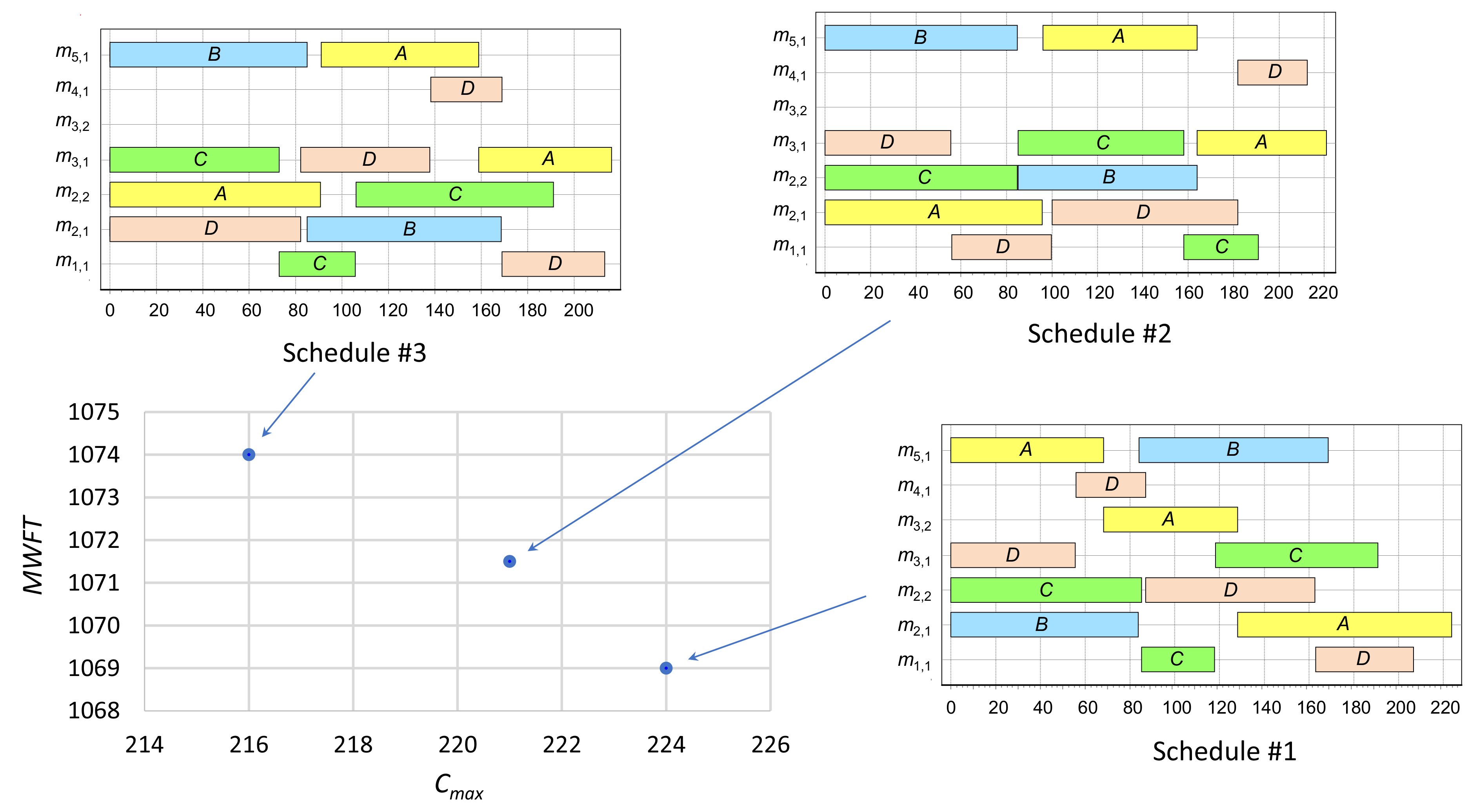
The corresponding MILP model is prepared using the OPL language [36] and is solved using IBM ILOG CPLEX version 12.8. The value of $\mathbb{M}$ is set to 10,000 and the value of $\delta$ is chosen to be 0.1. A total of four solver runs are needed to generate the set of non-dominated solutions, one using the DMOSP-CMAX model and three iterations using the DMOSP-MWFT($\epsilon$) model. Figure 1 shows the Gantt charts of the generated three non-dominated schedules. As demonstrated in Figure 1, despite the relatively small differences in the values of the two objective functions, the three schedules exhibit large discrepancies in the processing sequences on machines and job routes. Of course, the small differences in the values of the objective functions will accumulate over the scheduling periods affecting the system’s performance on the long run.

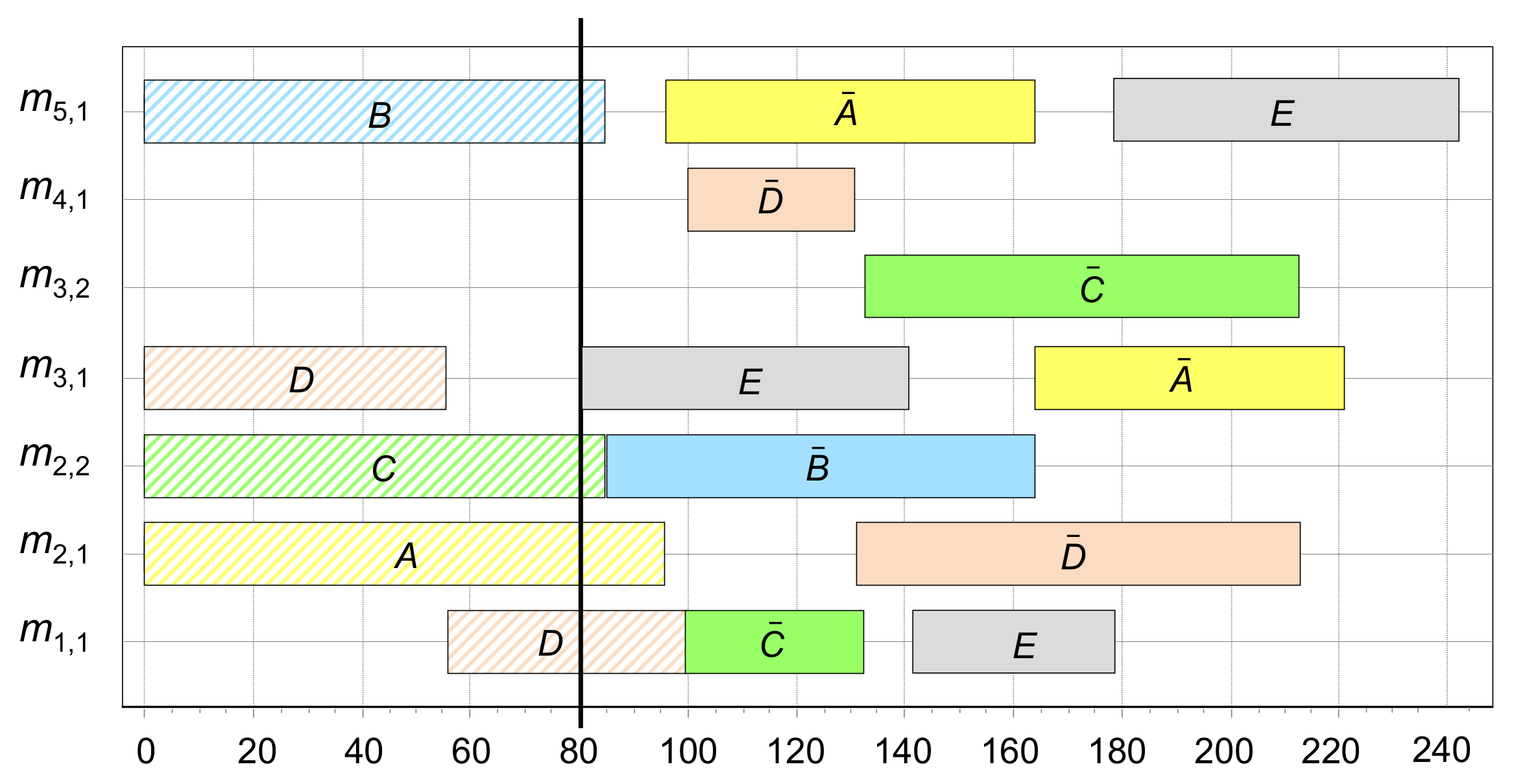
Next, we demonstrate how the developed model and the $\epsilon$-constraint algorithm can be used for guiding the rescheduling decisions whenever a new job arrives to the system during the execution of a selected schedule. Consider a situation in which the decision maker chooses “Schedule #2” from the set of the originally generated non-dominated schedules shown in Figure 1. A new job E arrives at time 80 which requires the processing on workstations 1, 3, and 5, and has a priority $p_E$ = 10. Assuming that the processing intervals provided by Schedule #2 are strictly followed with no deviation, the rescheduling problem can be formulated using the developed MILP model as follows. Since the processing of a job cannot be interrupted, the unfinished processes at time 80 will continue and their corresponding finish times define the machine available times. Meanwhile, the remaining operations that did not start yet at time 80 form a modified set of jobs which are denoted $\overline{A}$, $\overline{B}$, $\overline{C}$ and $\overline{D}$ and their priorities remain unchanged.

Table 2. Data for the rescheduling example after introducing job E at time 80 in the demonstrative example starting with Schedule #2 in Figure 1.

Jobs	Workstations
		1	2		3		4	5
		${\mathit{m}}_{\mathbf{1},\mathbf{1}}$	${\mathit{m}}_{\mathbf{2},\mathbf{1}}$	${\mathit{m}}_{\mathbf{2},\mathbf{2}}$	${\mathit{m}}_{\mathbf{3},\mathbf{1}}$	${\mathit{m}}_{\mathbf{3},\mathbf{2}}$	${\mathit{m}}_{\mathbf{4},\mathbf{1}}$	${\mathit{m}}_{\mathbf{5},\mathbf{1}}$
	${\mathbf{r}}_{\mathbf{j}}\setminus {\mathit{a}}_{\mathit{m}}$	100	96	85	80	80	80	85
$\overline{A}$	96				57	60		68
$\overline{B}$	85		84	79
$\overline{C}$	85	33			73	79
$\overline{D}$	100		82	76			31
E	80	38			61	67		63

shows the corresponding machine available times, job ready times, and the processing times for the rescheduling problem.

The $\epsilon$-constraint method is applied to the rescheduling problem. Three non-dominated schedules are generated with the following pairs of objective function values ($C_{max}$, $MWFT$): (257, 816), (252, 816.8), and (242, 826.8). If the decision maker opts to choose the schedule with the minimum makespan, the corresponding Gantt chart of the modified schedule is shown in Figure 2.

4. Results and Discussion

The main purpose of the computational experiments in this paper is to assess the performance of the developed exact algorithm in terms of the computational time requirements and to investigate the characteristics of the optimal Pareto front solutions of the studied problem. A total of 30 specially designed small instances are randomly generated and used in the current computations. These instances can be used as a testbed for future algorithmic developments.

In the designed instances, the number of workstations and the number of jobs are fixed at 5 and 10, respectively. The number of machines in a workstation is randomly generated from a discrete uniform distribution between 1 and 2. Job priority is randomly generated from a uniform distribution between 1 and 10. In the DMOSP structure, there is no restriction that a job has to visit all workstations. This is represented in the generated instances using a loading level ($LL$) factor, which represents the probability that a job visits a workstation during the instance generation. In the generated small instances, $LL$ is set equal to 0.7.

Processing times of jobs on machines are randomly generated as follows. First, for each workstation $w\in \mathcal{W}$, a nominal processing time, denoted ${\tilde{d}}_w$, is randomly generated from a uniform distribution between 30 and 50 multiplied by the number of machines in the workstation. For each machine $m\in M_w$, a processing time adjustment factor, denoted $PT{F}_m$, is randomly generated from a uniform distribution between 0.8 and 1.2. Accordingly, the processing time for job $j\in \mathcal{J}$ is determined as $d_{j,w,m}=⌈{\tilde{d}}_w\times PT{F}_m\times V_j⌉$, where $V_j$ is a randomly generated decimal number uniformly between 0.9 and 1.0 to represent the variability in the processing times among jobs.

Job release times are randomly generated using an average percentage of late jobs of 50%, which is realized by generating a decimal random number using uniform distribution between 0 and 1.0. If this decimal number is found to be below 0.5, the corresponding job’s release time is assigned a non-zero value. In such a case, $r_j=⌈RT{F}_j\times {\sum }_{w\in W_j}\left({\sum }_{M_w}{d}_{j,w,m}/\phantom{{\sum }_{M_w}{d}_{j,w,m}\left|M_w\right|}\left|M_w\right|\right)/\phantom{RT{F}_j\times {\sum }_{w\in W_j}\left({\sum }_{M_w}{d}_{j,w,m}/\phantom{{\sum }_{M_w}{d}_{j,w,m}\left|M_w\right|}\left|M_w\right|\right)\left|O_j\right|}\left|O_j\right|⌉$, where $RT{F}_j$ is a release time factor that is randomly generated from a uniform distribution between 0.2 and 2.

Similarly, machine available times are randomly generated using an average percentage of busy machines at the beginning of the schedule of 50%. In case a machine is randomly chosen to be busy, its available time is calculated as $a_m=⌈AT{F}_m\times {\tilde{d}}_w⌉$, where $AT{F}_m$ is the ready time factor for machine $m\in M_w$ in workstation w. Here, $AT{F}_m$ is randomly generated from a uniform distribution between 0.2 and 2.

Based on the selected ranges for the processing times generation scheme, it is found that the value of $\mathbb{M}=1000$ is sufficient for the validity of the constraints in the developed model. Since the generated job release times, machine available times, and processing times on machines are all integers, the value of $\delta$ is arbitrarily chosen as 0.9.

Computations using IBM ILOG CPLEX 12.8 are conducted on a laptop having an Intel Core i7-7550U central processing unit with a speed of 2.7 GHz and 8 GB physical memory under a Windows 10 operating system. The collected numerical measures are intended to be used to understand the shape of the optimal Pareto front as well as the computational time requirements.

4.1. Computational Time

Figure 3 illustrates the details of the computational times of the developed exact algorithm for the 30 instances. The $C_{max}$ time is the computational time needed for finding a proven optimal solution for the DMOSP-CMAX subproblem; meanwhile, the $MWFT$ time is the cumulative time spent for finding proven optimal solutions for all generated DMOSP-MWFT($\epsilon$) subproblems.

As shown in Figure 3, the computational time for the DMOSP-CMAX subproblem represents a small fraction of the total computational time needed to obtain the full optimal Pareto front. It exceeds 100 s only in four times; among them, for two different times, it exceeds 1000 s. For only six times, the total computational time exceeds the 10,000 s limit. If exceeding this limit is not practically acceptable, the CPLEX solver used for solving the subproblems generated within the developed exact algorithm can be terminated at an arbitrary intermediate time. This will result in an approximate solution that is not guaranteed to belong to the OPFs.

4.2. Characteristics of the Optimal Pareto Front

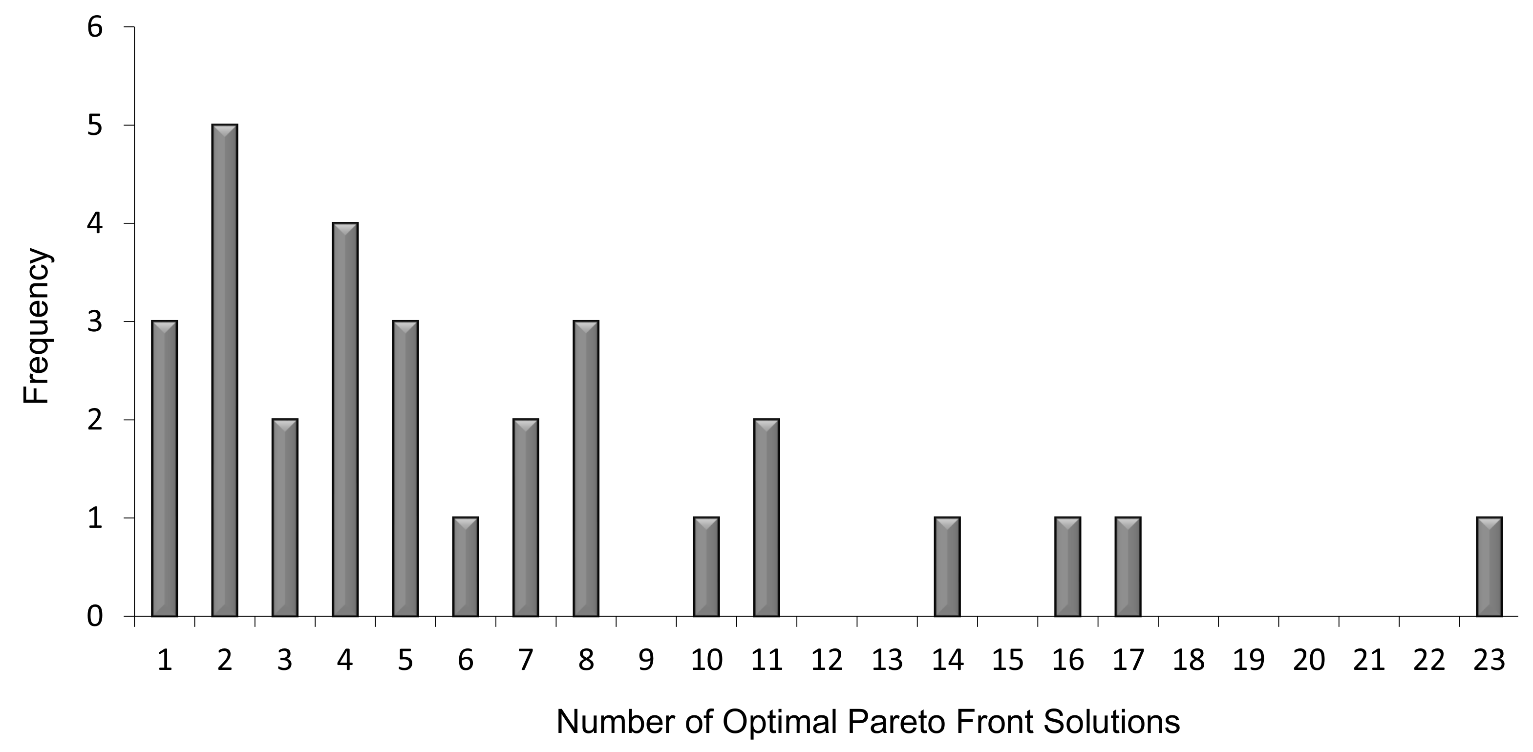
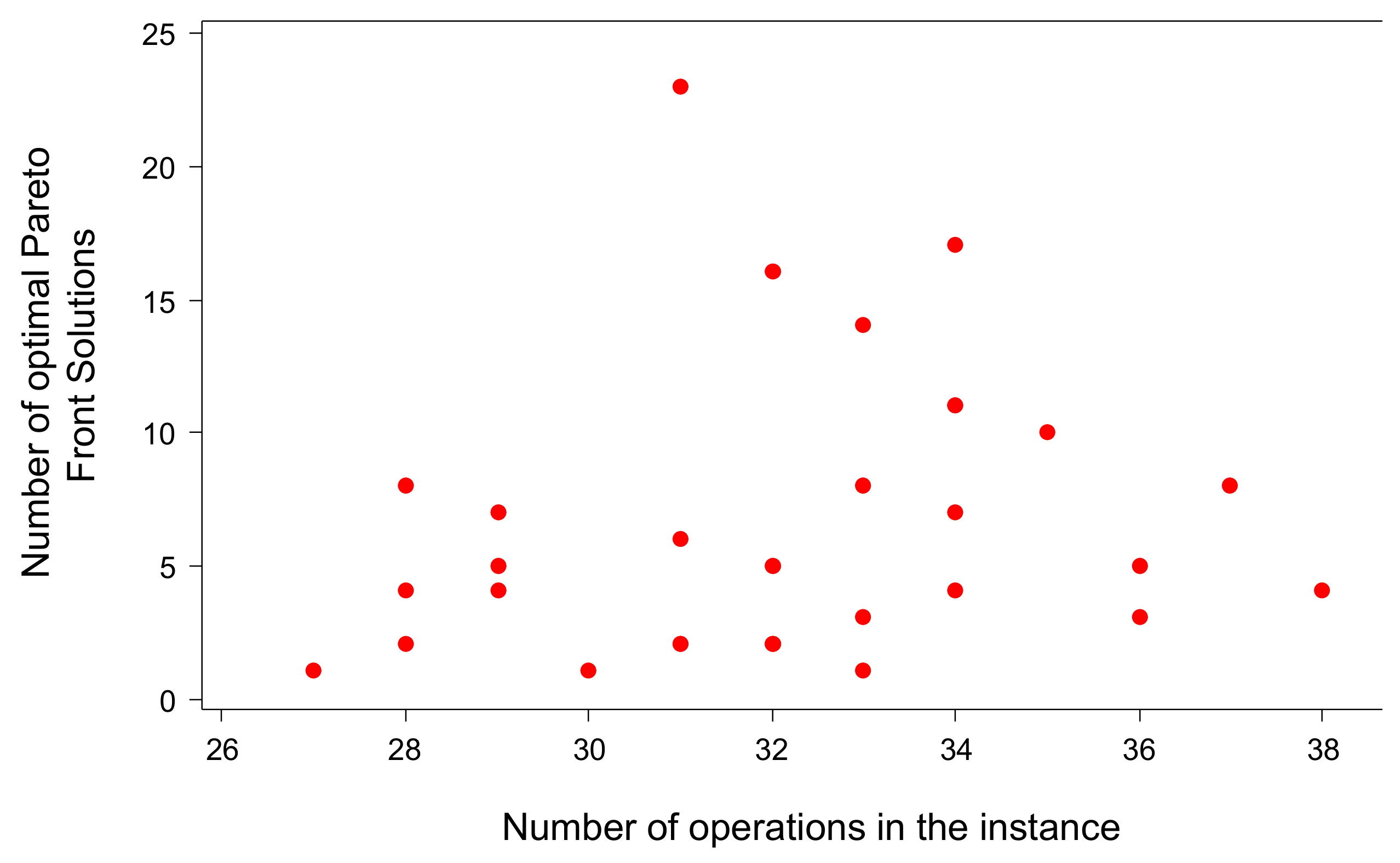
The number of optimal Pareto front solutions (OPFs) obtained for each instance is an important characteristic for the studied problem. Among the 30 instances, it is found that the number of OPF ranges from 1 to 23. Figure 4 presents the frequency distribution of the number of OPFs for the 30 instances. It is evident that there is a high level of variability in that number. However, having a median of 5 indicates that the number of OPFs is generally few. Meanwhile, there is no statistical evidence that the number of OPFs is correlated with the size of the instance represented by the total number of operations which ranges from 27 to 38 in the randomly generated instances as demonstrated by the scatter plot in Figure 5.

Another important characteristic is the wideness of the Pareto front which can be represented by the percentage difference between the maximum and the minimum values of both objective values for each instance. Dividing the wideness by the number of OPFs less than one provides an average indication of the spacing between solutions along the Pareto front for both objectives. This is referred to here as the spacing indicator. Therefore, for both objectives, the spacing indicators are evaluated as in Equations (15) and (16):

$$\begin{array}{cc}\hfill {\sigma }_{C_{max}}& =\frac{\underset{s\in \mathcal{P}}{max}\left\{C_{max}\left(s\right)\right\}-\underset{s\in \mathcal{P}}{min}\left\{C_{max}\left(s\right)\right\}}{\left(\left|\mathcal{P}\right|-1\right)\times \underset{s\in \mathcal{P}}{min}\left\{C_{max}\left(s\right)\right\}}\times 100\hfill \end{array}$$

(15)

$$\begin{array}{cc}\hfill {\sigma }_{MWFT}& =\frac{\underset{s\in \mathcal{P}}{max}\left\{MWFT\left(s\right)\right\}-\underset{s\in \mathcal{P}}{min}\left\{MWFT\left(s\right)\right\}}{\left(\left|\mathcal{P}\right|-1\right)\times \underset{s\in \mathcal{P}}{min}\left\{MWFT\left(s\right)\right\}}\times 100\hfill \end{array}$$

(16)

It is found that the spacing for the makespan (${\sigma }_{C_{max}}$) is mostly larger than the spacing for the MWFT (${\sigma }_{MWFT}$) in 22 instances and the opposite happens only in five instances.

Table 3. Descriptive statistics for the spacing indicators based on 27 instances.

Indicator	Mean	Std. Dev.	Minimum	First Quartile	Median	Third Quartile	Maximum
${\sigma }_{C_{max}}$	1.913	2.215	0.214	0.694	1.350	1.971	10.510
${\sigma }_{MWFT}$	0.5646	0.3687	0.1138	0.2742	0.4413	0.7204	1.3145

lists the descriptive statistics for both spacing indicators for 27 instances since only one optimal Pareto front solution is found in three instances, and, therefore, their corresponding values are excluded.

To the best of our knowledge, there is no standard reference to compare the spacing indicators of the OPFs of the DMOSP with. However, comparing the statistics for the two objective functions as summarized in Table 3 provides insights about the shape of the optimal Pareto front. The range, which is the difference between the maximum and the minimum observed values, is more than 8.5 times larger for ${\sigma }_{C_{max}}$ than ${\sigma }_{MWFT}$. Supported by the ratio of the standard deviation of ${\sigma }_{C_{max}}$ to that of ${\sigma }_{MWFT}$, it is evident that the Pareto front is more stretched in the direction of the makespan objective. For both spacing indicators, comparing the means with the median, first and third quartiles indicate that their distributions are skewed to the right. This means that the spacing indicators tend to have values that are relatively higher than the minimum reported values.

5. Conclusions and Future Research

This paper presented an exact solution algorithm for generating optimal Pareto front solutions for the dynamic multiprocessor open shop scheduling problem considering simultaneously the two objectives of minimizing the makespan and minimizing the mean weighted flow time. Both objectives are important in practical real-life applications. The developed exact algorithm is based on the $\epsilon$-constraint method. It utilizes CPLEX, a state-of-the-art MILP solver, for solving subproblems generated based on a developed MILP model. Computational experiments are conducted on a set of randomly generated 30 instances to assess the computational time requirements of the developed algorithm and to investigate the characteristics of the optimal Pareto front of the studied problem.

Computational time results demonstrated that the developed exact algorithm can be practically useful for instances having up to 10 jobs, five workstations, and one or two machines in a workstation. In 80% of the cases, the computational times were found to be less than 10,000 s. In some real-life applications, such a computational time limit can be acceptable if the time span of running the schedule itself is over a few days. Alternatively, instead of generating the optimal Pareto front solutions, the CPLEX solver can be terminated at a pre-specified time limit. This will result in approximate solutions that are not proven to be optimal, yet they represent a good approximation of the optimal Pareto front. This adaptation allows the utilization of the developed exact algorithm as an approximate approach.

Regarding the characteristics of the optimal Pareto front of the studied problem, computational results revealed that the size of the optimal Pareto front is small as it is composed of a small number of six to seven solutions on average. No evidence is found for the correlation between the size of the problem instance represented by the number of operations and the number of optimal Pareto front solutions. This result indicates that future algorithmic approaches need to pay more attention to intensification strategies as opposed to obtaining dense non-dominated solutions. This may contradict the traditional intention of multi-objective metaheuristic approaches that look for having a large “volume” of non-dominated solutions. Generally, intensification can be achieved by well-designed neighborhood search functions that are capable of improving solutions in both directions of the considered objective functions.

In addition, computational results show that the optimal Pareto front is more stretched in the direction of the makespan objective by having larger distances between every pair of consecutive solutions along the Pareto front compared to the mean weighted flow time objective. This characteristic may imply that more attention needs to paid to algorithmic techniques that seek to improve the MWFT objective to be able to deal with the small distances in that direction.

Future metaheuristic developments for the studied problem can benefit from recent population management structures such as the use of a reference set and the adaptive hybrid mutation operation which can be effectively used to manage neighborhood search functions in evolutionary based metaheuristics as demonstrated by Chen et al. [37].

References

- Pinedo, M. Scheduling: Theory, Algorithms, and Systems; Springer: Berlin, Germany, 2012. [Google Scholar]
- Werner, F.; Burtseva, L.; Sotskov, Y.N. Special Issue on Algorithms for Scheduling Problems. Algorithms 2018, 11, 87. [Google Scholar] [CrossRef] [Green Version]
- Werner, F.; Burtseva, L.; Sotskov, Y.N. Special Issue on Exact and Heuristic Scheduling Algorithms. Algorithms 2019, 13, 9. [Google Scholar] [CrossRef] [Green Version]
- Uhlmann, I.R.; Frazzon, E.M. Production rescheduling review: Opportunities for industrial integration and practical applications. J. Manuf. Syst. 2018, 49, 186–193. [Google Scholar] [CrossRef]
- Hwang, C.L.; Masud, A.S.M. Multiple Objective Decision Making—Methods and Applications: A State-of-the-Art Survey; Springer: Berlin/Heidelberg, Germany, 1979; Volume 164. [Google Scholar] [CrossRef]
- Graham, R.; Lawler, E.; Lenstra, J.; Rinnooy Kan, A. Optimization and approximation in deterministic sequencing and scheduling: A survey. Ann. Discret. Math. 1979, 5, 169–231. [Google Scholar]
- Vignier, A.; Billaut, J.C.; Proust, C. Les flowshop hybrides: état de l’art (in French). RAIRO-Oper. Res. 1999, 33, 117–183. [Google Scholar] [CrossRef]
- Gonzalez, T.; Sahni, S. Open Shop Scheduling to Minimize Finish Time. J. ACM 1976, 23, 665–679. [Google Scholar] [CrossRef]
- Achugbue, J.O.; Chin, F.Y. Scheduling the open shop to minimize mean flow time. SIAM J. Comput. 1982, 11, 709–720. [Google Scholar] [CrossRef]
- Seraj, O.; Tavakkoli-Moghaddam, R.; Jolai, F. A fuzzy multi-objective tabu-search method for a new bi-objective open shop scheduling problem. In Proceedings of the 2009 International Conference on Computers Industrial Engineering, Troyes, France, 6–8 July 200; pp. 164–169. [CrossRef]
- Sha, D.Y.; Lin, H.H.; Hsu, C.Y. A Modified Particle Swarm Optimization for Multi-objective Open Shop Scheduling. In Proceedings of the International MultiConference of Engineers and Computer Scientists 2010 (IMECS 2010), Hong Kong, China, 17–19 March 2010; Volume III. [Google Scholar]
- Tavakkoli-Moghaddam, R.; Panahi, H.; Heydar, M. Minimization of weighted tardiness and makespan in an open shop environment by a novel hybrid multi-objective meta-heuristic method. In Proceedings of the 2008 IEEE International Conference on Industrial Engineering and Engineering Management, Singapore, 8–11 December 2008; pp. 379–383. [Google Scholar] [CrossRef]
- Panahi, H.; Tavakkoli-Moghaddam, R. Solving a multi-objective open shop scheduling problem by a novel hybrid ant colony optimization. Expert Syst. Appl. 2011, 38, 2817–2822. [Google Scholar] [CrossRef]
- Naderi, B.; Mousakhani, M.; Khalili, M. Scheduling multi-objective open shop scheduling using a hybrid immune algorithm. Int. J. Adv. Manuf. Tech. 2013, 66, 895–905. [Google Scholar] [CrossRef]
- Schuurman, P.; Woeginger, G.J. Approximation algorithms for the multiprocessor open shop scheduling problem. Oper. Res. Lett. 1999, 24, 157–163. [Google Scholar] [CrossRef] [Green Version]
- Jansen, K.; Sviridenko, M. Polynomial Time Approximation Schemes for the Multiprocessor Open and Flow Shop Scheduling Problem. In STACS 2000; Reichel, H., Tison, S., Eds.; Springer: Berlin/Heidelberg, Germany, 2000. [Google Scholar] [CrossRef]
- Sevastianov, S.; Woeginger, G. Linear time approximation scheme for the multiprocessor open shop problem. Discret. Appl. Math. 2001, 114, 273–288. [Google Scholar] [CrossRef] [Green Version]
- Naderi, B.; Fatemi Ghomi, S.; Aminnayeri, M.; Zandieh, M. Scheduling open shops with parallel machines to minimize total completion time. J. Comput. Appl. Math. 2011, 235, 1275–1287. [Google Scholar] [CrossRef]
- Goldansaz, S.M.; Jolai, F.; Zahedi Anaraki, A.H. A hybrid imperialist competitive algorithm for minimizing makespan in a multi-processor open shop. Appl. Math. Model. 2013, 37, 9603–9616. [Google Scholar] [CrossRef]
- Abdelmaguid, T.F. Scatter search with path relinking for multiprocessor open shop scheduling. Comput. Ind. Eng. 2020, 141, 106292. [Google Scholar] [CrossRef]
- Matta, M.E. A genetic algorithm for the proportionate multiprocessor open shop. Comput. Oper. Res. 2009, 36, 2601–2618. [Google Scholar] [CrossRef]
- Abdelmaguid, T.F.; Shalaby, M.A.; Awwad, M.A. A tabu search approach for proportionate multiprocessor open shop scheduling. Comput. Optim. Appl. 2014, 58, 187–203. [Google Scholar] [CrossRef]
- Abdelmaguid, T.F. A Hybrid PSO-TS Approach for Proportionate Multiprocessor Open Shop Scheduling. In Proceedings of the 2014 IEEE International Conference on Industrial Engineering and Engineering Management (IEEM), Bandar Sunway, Malaysia, 9–12 December 2014; pp. 107–111. [Google Scholar]
- Zhang, J.; Wang, L.; Xing, L. Large-scale medical examination scheduling technology based on intelligent optimization. J. Combin. Optim. 2019, 37, 385–404. [Google Scholar] [CrossRef]
- Bai, D.; Zhang, Z.H.; Zhang, Q. Flexible open shop scheduling problem to minimize makespan. Comput. Oper. Res. 2016, 67, 207–215. [Google Scholar] [CrossRef]
- Wang, Y.T.H.; Chou, F.D. A Bi-criterion Simulated Annealing Method to Solve Four-Stage Multiprocessor Open Shops with Dynamic Job Release Time. In Proceedings of the 2017 International Conference on Computing Intelligence and Information System (CIIS), Nanjing, China, 21–23 April 2017; pp. 13–17. [Google Scholar] [CrossRef]
- Abdelmaguid, T.F. An Efficient Mixed Integer Linear Programming Model for the Minimum Spanning Tree Problem. Mathematics 2018, 6, 183. [Google Scholar] [CrossRef] [Green Version]
- Bowman, E.H. The Schedule-Sequencing Problem. Oper. Res. 1959, 7, 621–624. [Google Scholar] [CrossRef]
- Wagner, H.M. An integer linear-programming model for machine scheduling. Nav. Res. Logist. Q. 1959, 6, 131–140. [Google Scholar] [CrossRef]
- Manne, A.S. On the Job-Shop Scheduling Problem. Oper. Res. 1960, 8, 219–223. [Google Scholar] [CrossRef] [Green Version]
- Stafford, E.F.; Tseng, F.T.; Gupta, J.N. Comparative evaluation of MILP flowshop models. J. Oper. Res. Soc. 2005, 56, 88–101. [Google Scholar] [CrossRef]
- Naderi, B.; Fatemi Ghomi, S.; Aminnayeri, M.; Zandieh, M. A study on open shop scheduling to minimise total tardiness. Int. J. Prod. Res. 2011, 49, 4657–4678. [Google Scholar] [CrossRef]
- Demir, Y.; Kürşat Işleyen, S. Evaluation of mathematical models for flexible job-shop scheduling problems. Appl. Math. Model. 2013, 37, 977–988. [Google Scholar] [CrossRef]
- Ku, W.Y.; Beck, J.C. Mixed Integer Programming models for job shop scheduling: A computational analysis. Comput. Oper. Res. 2016, 73, 165–173. [Google Scholar] [CrossRef] [Green Version]
- Mavrotas, G. Effective implementation of the ϵ-constraint method in Multi-Objective Mathematical Programming problems. Appl. Math. Comput. 2009, 213, 455–465. [Google Scholar] [CrossRef]
- Van Hentenryck, P. The OPL Optimization Programming Language; MIT Press: Cambridge, MA, USA, 1999. [Google Scholar]
- Chen, M.R.; Zeng, G.Q.; Lu, K.D. A many-objective population extremal optimization algorithm with an adaptive hybrid mutation operation. Inform. Sci. 2019, 498, 62–90. [Google Scholar] [CrossRef]
Figure 1.
Optimal Pareto front and the Gantt charts of the corresponding schedules for the demonstrative example.
Figure 2.
Gantt chart of the updated schedule after introducing job E at time 80 in the demonstrative example starting with Schedule #2 in Figure 1.
Figure 3.
Computational times for the 30 instances.
Figure 4.
A histogram showing the frequency distribution of the number of optimal Pareto front solutions.
Figure 5.
A scatter plot for the number of optimal Pareto front solutions versus the size of the instance.