Study of Quasi-Static Magnetization with the Random-Field Ising Model


Department of Semiconductor and Optoelectronics Devices, Lodz University of Technology, Wólczańska Str. 211/215, 90-924 Łódź, Poland
Algorithms 2020, 13(6), 134; https://0-doi-org.brum.beds.ac.uk/10.3390/a13060134
Submission received: 15 April 2020
/
Revised: 22 May 2020
/
Accepted: 25 May 2020
/
Published: 29 May 2020
(This article belongs to the Special Issue Algorithms for Diagnostics and Nondestructive Testing)
Abstract
:The topic of this paper is modeling based on Hamiltonian spin interactions. Preliminary studies on the identification of quasi-static magnetizing field in a magnetic system were presented. The random-field Ising model was then used to simulate the simplified ferromagnetic structure. The validation of algorithms and simulation tests were carried out for the 2D and the 3D model spaces containing at least 106 unit cells. The research showed that the response of a slowly driven magnetic system did not depend on the external field sweep rate. Changes in the spatial magnetization of the lattice were very similar below a certain rate of the external field change known as the quasi-static boundary. The observed differences in obtained magnetization curves under quasi-static conditions stemmed from the random nature of the molecular field and the avalanche-like magnetization process
1. Introduction
The concept of a cellular automaton was introduced by Ulam and Von Neumann [1,2]. At present, cellular automata are used as a scientific tool in studies of complex dynamic systems, microstructures, and many other applications [3,4,5,6,7]. Cellular automaton (CA) is an example of how simple rules and local interactions can lead to very diverse and complicated behaviors [8,9]. Usually, cellular automata are simple and regular grids. Each node of the grid is in a defined discrete state. The states of the nodes are updated synchronously at discrete moments and the state of each node at the next moment is a function of the state of its neighbors in the current moment. The Ising model, being a magnetic system based on statistical mechanics, is a magnificent example of a cellular automaton that was developed much earlier than the aforementioned cellular automaton concept [10,11]. The model is widely used in computer physics for the analysis of magnetic hysteresis [12,13] phase transitions [14,15], dynamics of magnetization [16,17], Barkhausen noise [13,15,17,18], and energy loss in magnetic materials [19], as well as for defect and inhomogeneity studies in magnetic structures [20,21,22,23,24,25].
Magnetic modeling using the interactions of so-called “spins” arranged in a lattice of regular unit cells is the most widely used approach. A single spin can be interpreted as a magnetic moment of an atom in a crystal lattice, crystal grain, magnetic domain, or quantized amorphous space [26]. Modeling of spontaneous magnetization processes including hysteresis, displacements of domain walls, and the Barkhausen effect are some of the common applications of the Ising model [26,27,28]. The vast majority of works use the random-field Ising model (RFIM) based on the Hamiltonian as the energy function with an additional term representing the random molecular magnetic field assigned to each spin [13,14,29,30].
However, the RFIM does not explicitly take into account the time scale. Therefore, the simulation results are qualitatively and quantitatively consistent only for time-independent processes such as the primary magnetization curve or the static magnetic hysteresis loop [28].
Studies of hysteresis in soft magnetic materials have always been a part of scientific work. Various magnetic, physical, structural, thermodynamic, and many other parameters are identified on the basis of the shape and area of the hysteresis loop. Basically, loops can be classified as static or dynamic [12,31], but the magnetizing field must be variable over time to obtain both hysteresis loops. The static loop is interesting because it illustrates the magnetizing process without time-dependent effects. In practice, the change in material magnetization is quite complex and there is no strict interpretation when the process can be considered static, even when an extremely low frequency sweep rate is used [6,32]. Therefore, this approach shall only be considered as a quasi-static approximation of a boundary static process [32]. Many works on testing magnetic materials arbitrarily assume, without any explanation, that the frequency sweep rate is low enough that, e.g., eddy currents may be neglected. The real limitation of the static condition results very often from the technical limitations of the measuring instruments. In this case, one cannot assess how large the discrepancy of such an approximation is. In this context, the paper provides a contribution in the field of slowly driven magnetic systems through the identification of the quasi-static limiting of magnetization processes in magnetic materials. Coliaori et al. [19] showed the dependency of field sweep rate in the RFIM on the coercive field of magnetic thin films and pointed out a direct link between the theory of loss separation for bulk materials and a simple magnetic system with disorder. Thus, the aim of this work is to check if RFIM, as a mathematical model of ferromagnetism, shows a tendency to reach the limit of quasi-static magnetization under general conditions.
2. Random-Field Ising Model
The model space is defined as a set of unit cells associated with the Szi spin operators. Spins denoted as Szi are surrounded by j = 2D adjacent spins Szj. The Szi spin is coupled with Szj through exchange interactions. Spin operators take values from the set of Szi, Szj = { −1, +1} and change the values to the opposite by spin flip.
A set of periodically arranged unit cells creates either a spatial or a flat model lattice with spins placed in all sites of the lattice. The number of spins in the model space depends on the form of the unit cell, the number of space dimensions D and the lattice length L for each dimension. The unit cell is here referred to as a site in the lattice. The model space is therefore defined as the D-dimensional lattice of regular unit cells limited in each direction by its pertinent length LD, and comprising N sites with localized spins (Equation (1)).
Other magnetic structures require consideration of both other forms of unit cells and other numbers of localized spins coupled by exchange interactions [20,27]. The use of regular cells instead of more complicated forms is a typical simplification of the model space. In other cases, when the structure is not a crystal lattice or has a very heterogeneous form, one can quantize the space with regular cells and estimate equivalent parameters. The fundamental Hamiltonian form of the Ising model takes into account both the exchange interactions between the nearest-neighbored spins in the lattice and the applied external field H. The Hamiltonian of the RFIM (Equation (2)) imposes quenched disorder in the form of a random molecular field hi assigned to all sites i of the lattice [26].
The value of the hi field in Equation (2) has an impact only on triggering the spin Szi flip induced either by adjacent spins Szj or by the external field H [28]. Parallel polarization of all spins in the lattice occurs under the influence of exchange interactions in the Weiss molecular field [12,13]. In the RFIM, the subsequent values of the hi field are random variables and depend on the parameters of the random distribution described by Equation (3).
The set of random values hi ∈ {h0, h1, … hN-1} is generated on the basis of the Gaussian distribution function described by the relationship in Equation (3) and is additionally subject to the limitations defined by Equation (4). The mean value of the set hi in the space defined by N spins tends to zero (Equation (4)). Variance of random fields hi is a function of the disorder R at the temperature T ~0 K.
The range of changes in the parameter R is limited by the value of critical disorder Rc [13,28]. The sequence of random hi ∈ {h0, h1, … hN-1} for R > Rc may contain hi elements that do not guarantee the convergence of the simulation process (non-ergodic sequence of random variables) [29]. A more comprehensive analysis of the disorder parameter in the RFIMs was carried out in works [15,17,18,26,28]. If the effective field heff (Equation (5)) acting in a given site i changes the sign to the opposite, then flipping of the Szi spin occurs and its value is also changed to the opposite.
The flip condition (Equation (6)) may occur if there is either a change in the configuration of adjacent spins Szj for a given instantaneous value of field H, or a change in the instant value of the magnetizing field H with a fixed configuration of spins Szj.
The initial equilibrium of the model is achieved at a temperature close to absolute zero (with no thermal fluctuations, accidental spin excitations, changes in spontaneous magnetization saturation): Ms (T = 0, H = 0). Evolution from the initial equilibrium state to the subsequent equilibrium or metastable states takes place in the magnetization process, forced by a homogeneous, external H field. The estimation of average magnetization during metastable magnetization states (H, m = const) is based on the relationship in Equation (7),
Where Szi+ denotes spins that have been flipped and Szi- spins that remain in their initial configuration. To estimate the area of the model space where unstable changes in magnetization are induced, the correlation function (Equation (8)) of x number of spin flips denoted as x and random field disorder R was used [13,26,28].
The estimation of the G value for a given R indicates the dynamics of magnetization and shows changes in the number of correlated spin flips (avalanches) triggered by a single spin flip.
3. Numerical Implementation
Numerical implementation of the RFIM involves the algorithms for generation of pseudo-random numbers and collective spin flipping.
To determine the sequence of random fields hi, the three-stage random number generator was used. In the first step, a start sequence of five pseudo-random values initiated the relevant generator. The initial set was generated by a linear congruential generator for a given seed value [33]. Next, a sequence of pseudo-random numbers from the range (0,1) was generated on the basis of the Tausworth algorithm [34]. In the third stage, one random variable with a Gaussian distribution was calculated from the two previously generated independent variables of the even distribution by means of the Box–Muller method [33,35]. The output value was scaled according to the determined standard deviation specified by the disorder R. All Szi spins were set to −1 and random values hi are assigned to them. The initial value of the external field Hmin < min(hi) was determined.
Avalanche spin flipping was triggered by increasing gradually the external field with a step ΔH. The condition (Equation (5)) of spin flip was checked by the brute force linear search method [18]. The algorithm is not very effective numerically, but allows one to determine explicitly the instantaneous changes in spatial magnetization and map other parameters of the model. The space was searched as long as all spins for the given external field H could be flipped. In the next step, the external field Hi+1 = Hi + ΔH was again increased and the subsequent step of the search algorithm was executed. The procedure was repeated until all spins in the entire model space were flipped (Equation (6)).
4. Results and Discussion
Numerical simulations using RFIM were carried out to verify the Gaussian pseudo-random number generator and spin flip procedure. Subsequently, the dynamics of the magnetization process of 2D and 3D structures was examined.
Model verification included both the discrepancies in the average value of the generated pseudo-random set hi according to dependencies 3 and 4 and the correlation of the spin flip process G (x, R) depending on the set of pseudo-random parameter values using the correlation functions (Equations (8) and (9)).
Analyzing the changes in the average value of the hi parameters against the size of the model space N for various values of the disorder R (Figure 1), one can assume that these changes are negligibly small in comparison with the hi values for the model space comprising above N = 104 spins. However, if the value N falls below 104, one should either consider the non-equilibrium magnetization state resulting from the non-zero mean hi or reduce the discussed problem by increasing the size of the model space so that the number of spins would exceed 104. Thus, the reduced impact of the non-equilibrium initial state occurs in simulations of two-dimensional spaces (D = 2) for the values of the parameter L > 100, and L > 22 in the case of the three-dimensional model (D = 3).
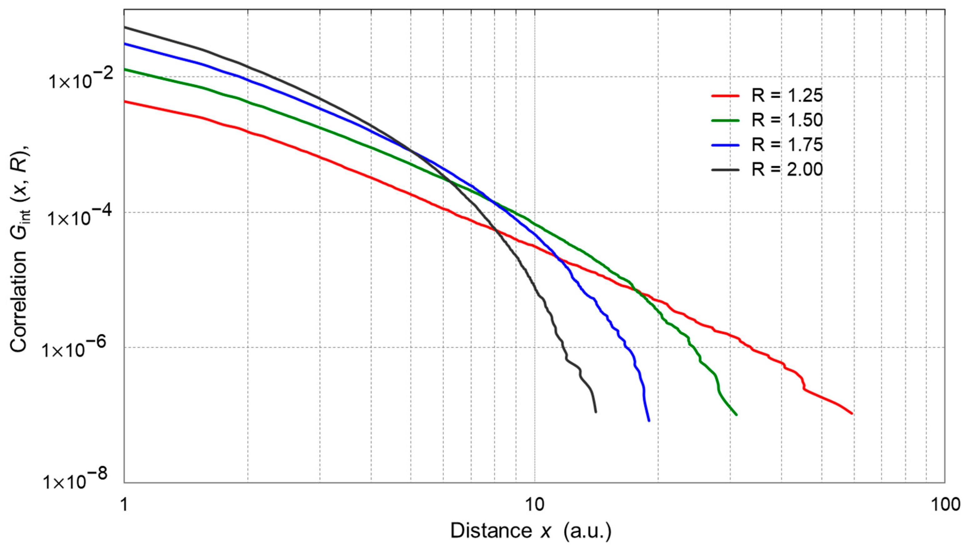
Another tested parameter of the model was the correlation of spin flips in areas of the model where avalanche processes occurred. The effect of avalanches, which introduce discontinuous changes in the magnetization of the model space, was determined on the basis of Equation (9). It can therefore be assumed that the discrete states of magnetization, recorded in the course of simulation, also strongly depend on the correlation of spin flips. The value of spin flip correlation can be estimated by determining the distance x (avalanche size) defined as the number of sites of inverted spins relative to the spin starting the avalanche process. Based on the normalized number of classes, range width, and class limits, the histogram of correlated inversions was determined in accordance with the relationships found in Equations (8) and 9). A graph of the spin flip correlation function was created by accumulating number of flipped spins in class intervals for a given distance x of correlated spin interactions (Figure 2) The high variability of the spin flip correlation function indicated that avalanches were nucleated frequently [13,30], but their propagation was often quenched by fluctuations of random fields hi. The size of avalanches depended on the value of disorder introduced to the model space.
Test results of the developed pseudo-random number generator (PRNG) showed that the numerical performance of the generator did not introduce significant limitations associated with simulation time. The implementation efficiency of the PRNG algorithm at 107 numbers per second was sufficient for the RFIM model, because the simulation did not require the generation of pseudo-random numbers ad hoc. Considering the limitations related to the mean value of the hi set, it should be stated that the model space with 106 spins guarantees the correct convergence of computer simulations [26,27].
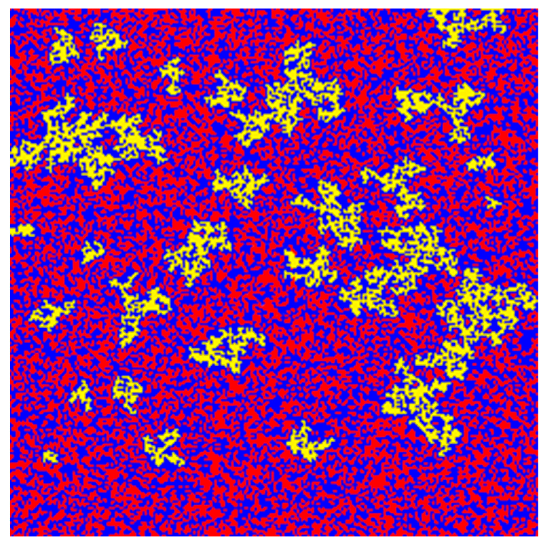
The developed algorithm of a three-stage pseudo-random generator (Section 3) led to the formation of clusters. These were areas where the directly coupled spins had random values of hi and the same sign. Clusters can introduce a weak effect of collective interactions. It is very likely that all spins in a cluster will be flipped in the same simulation step. Clusters are able to boost occurring avalanches or trigger the new ones. Figure 3 shows the distribution of random fields with the same sign over the 2D model space. Additionally, the exemplary clusters are highlighted.
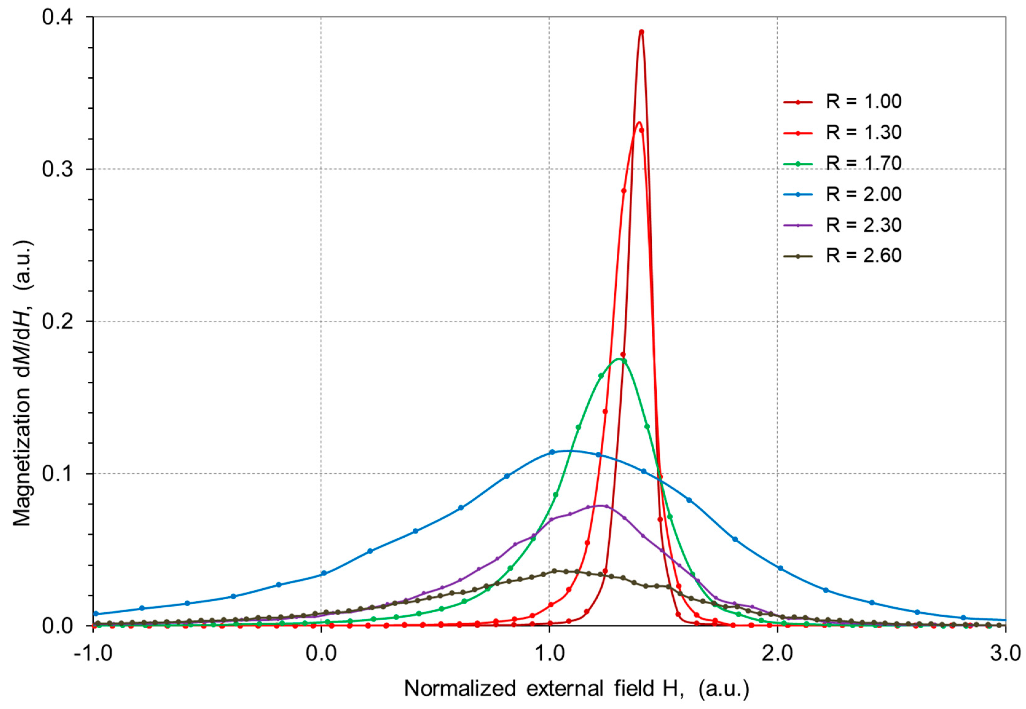
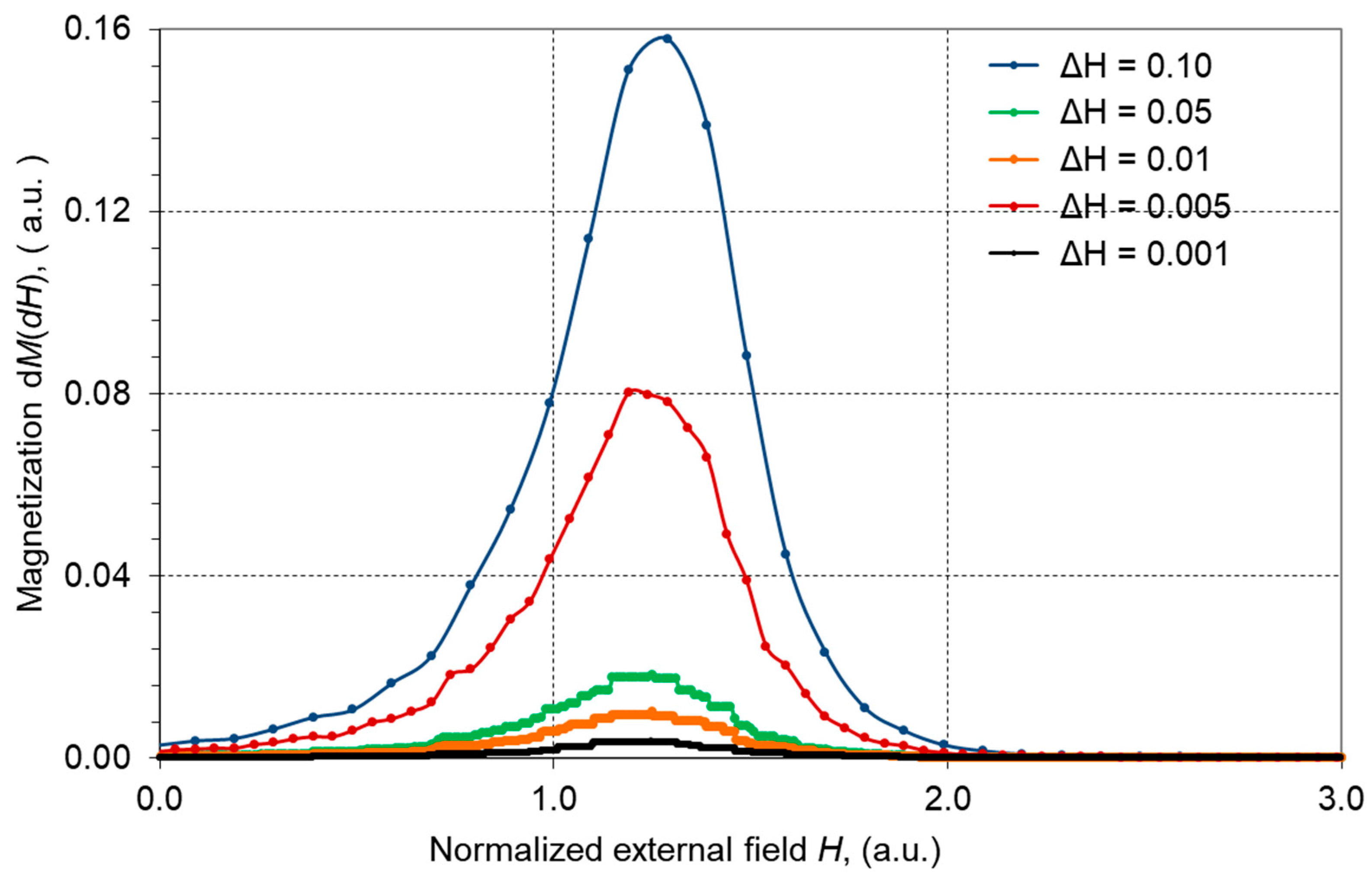
The impact of both the disorder and the range of variation of the disorder parameter R on magnetization were examined. The magnetizing process depending on the disorder parameter R was depicted in graphs of meta-stable magnetization changes dM/dH (Figure 4 and Figure 5) and hysteresis loops (Figure 6).
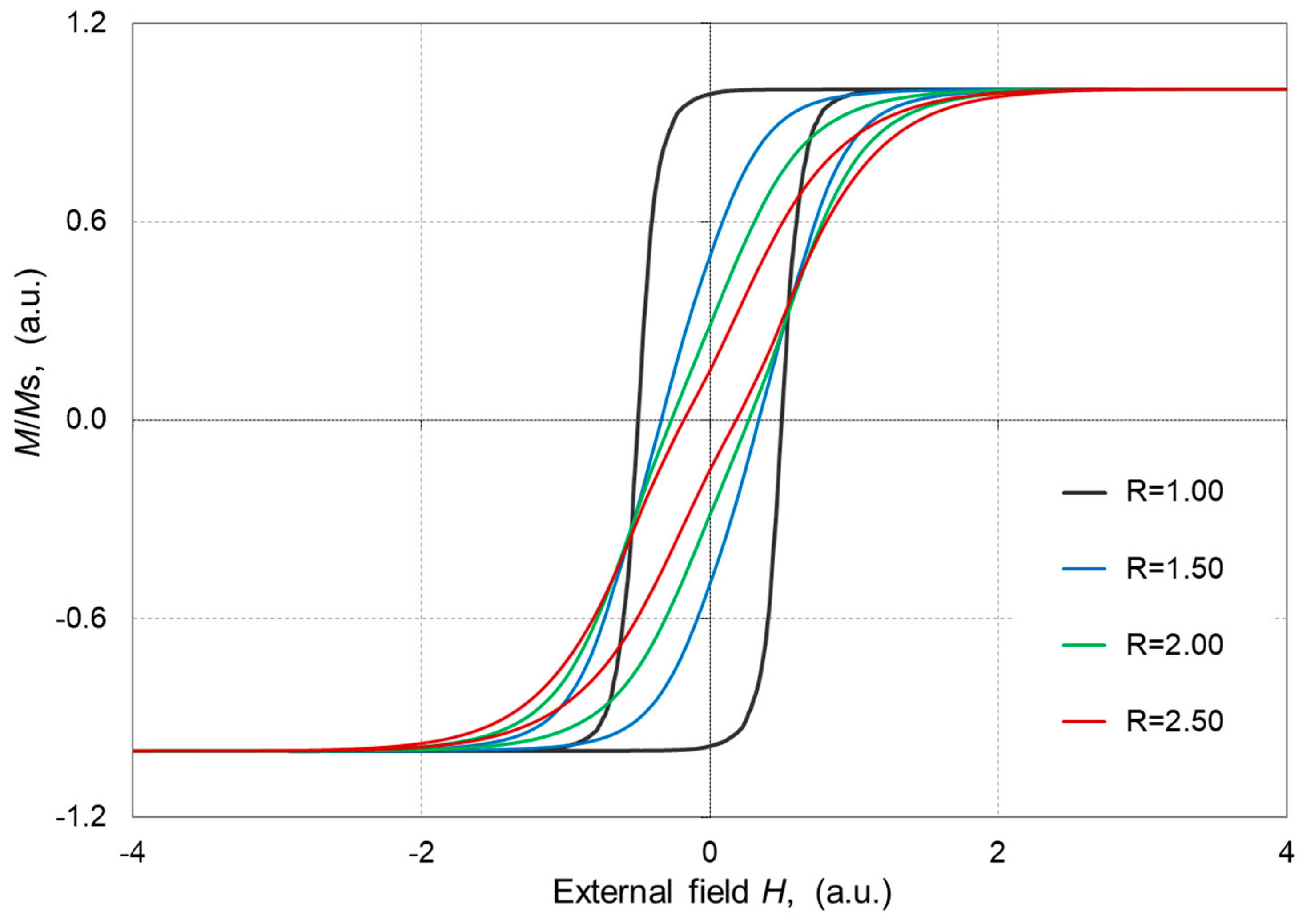
A greater magnetic order of the magnetic system and thus a smaller standard deviation of the random field component in each site of the model space affected the exchange energy of the localized spins in the considered site. The ratio of the strength of exchange interactions to the random field hi was greater, and therefore the energy needed to overcome the magnetic order in each site was also greater. Therefore, the coercive field was the highest when the influence of the random field component in the model space was the lowest. A magnetic system with higher disorder tends to lower magnetic susceptibility and reduces the coercive field as well [19]. Hence, smooth hysteresis loops significantly depend on the symmetrical shape of the hi distribution rather than the nearest neighbor interactions.
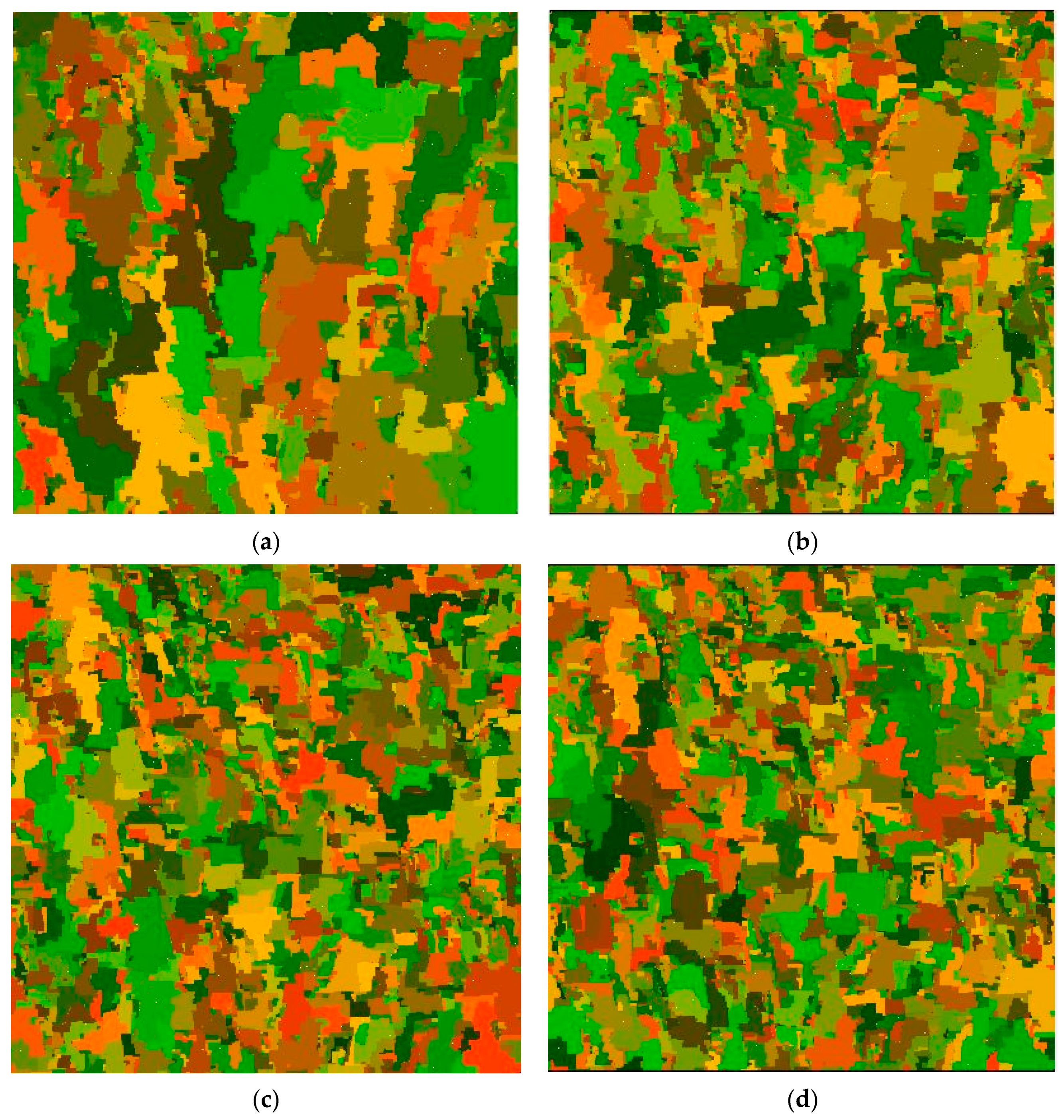
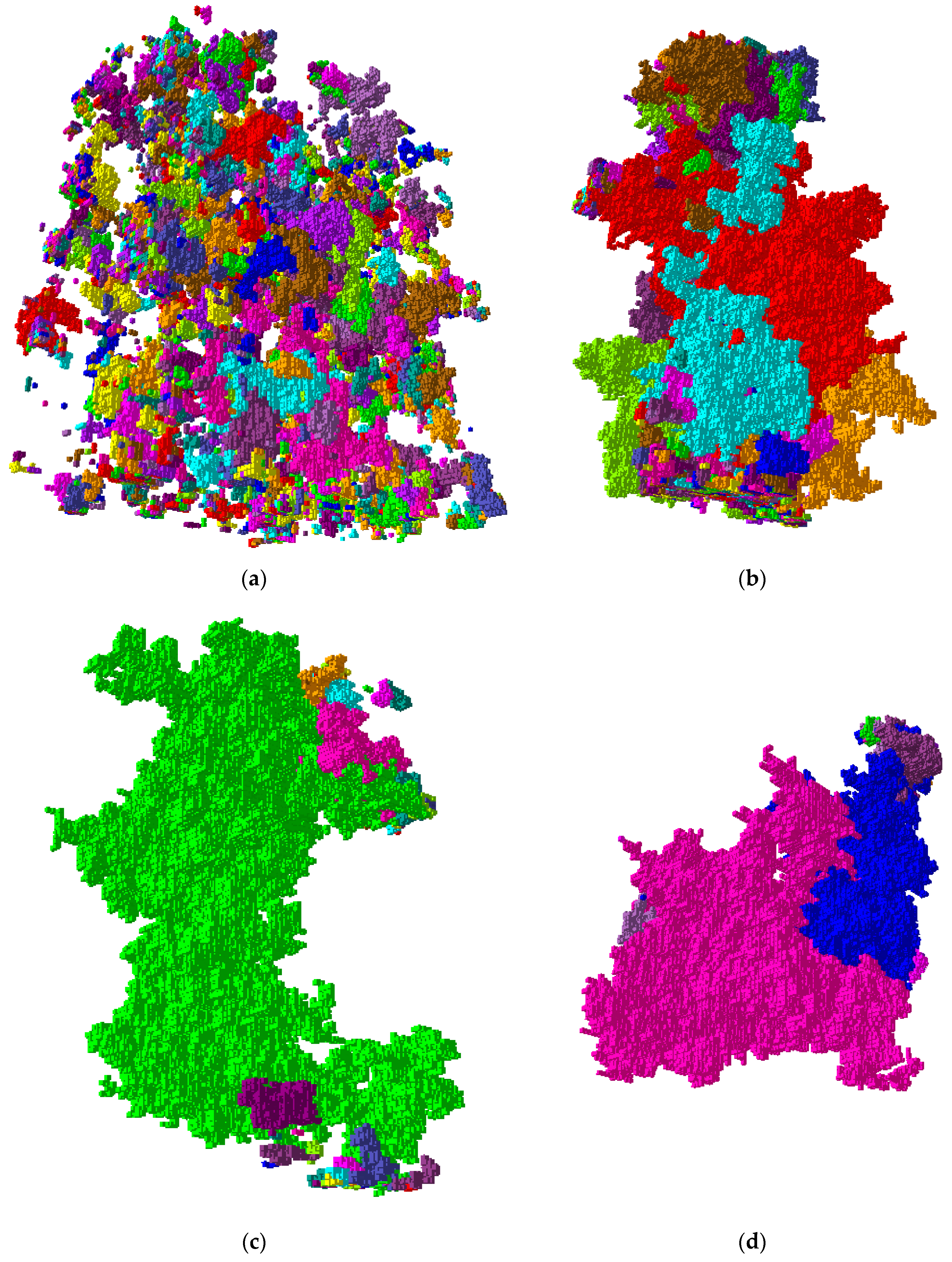
Figure 7a–d and Figure 8a–d respectively present mapping of the 2D and the 3D metastable states of magnetization due to spin flipping. Single-colored areas (the colors are attributed randomly) refer to regions in which the magnetization processes were avalanche-like. Flip of spins in these areas occurred under conditions of the temporarily determined value of the external field H. Each single spin flip for a given field value was marked with the same color of pixels/cubes on the 2D and 3D maps.
Simulations of the quasi-static process were performed in the same way as earlier tests of numerical implementation efficiency of the RFIM model. A single-spin flip method and a sorting algorithm were used to identify spins meeting the conditions described by the relationships 5 and 6.
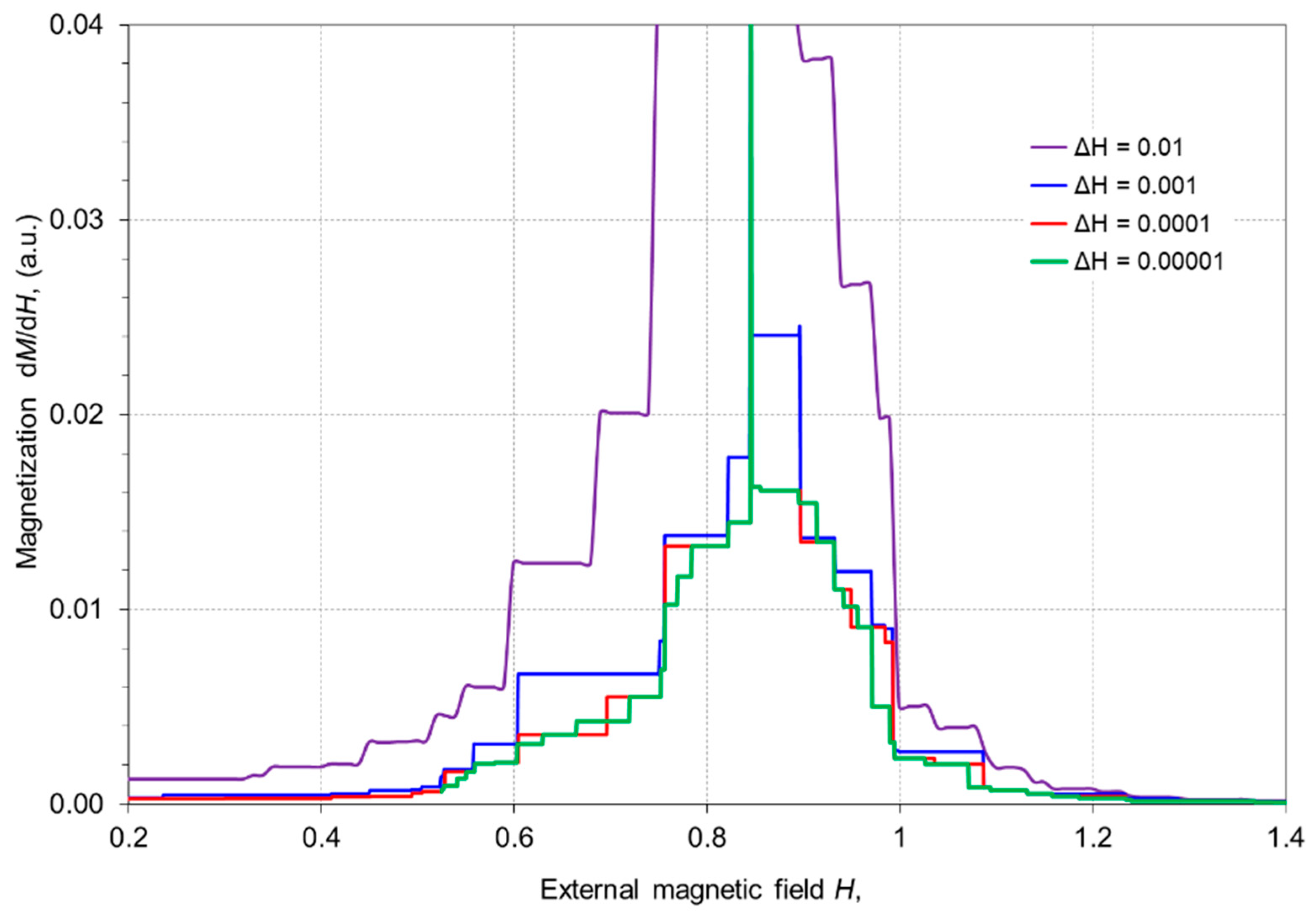
The quasi-static magnetization process, almost independent of the external field step rate, is depicted in Figure 9. Hence, it is possible to achieve a similar course of metastable changes in magnetization triggered by an external field with a different rate of change. Similar shapes of avalanches presented in Figure 7c,d also may prove the quasi-static magnetization process. The observed damping of the metastable changes in magnetization was generally consistent with experimental data [12] (Vol.II, Ch.3). The small increment of the external field H had a negligible impact on the occurring avalanche-like changes in magnetization. The avalanche of spin flips caused discrete changes in magnetization called the Barkhausen effect [15,27]. The greatest impact of the spin-flip avalanche on the change of magnetization was observed in simulations with moderate disorder R∈<1.0, 2.0> of random field hi.
5. Conclusions
The RFIM model was applied for the numerical studies on slowly driven magnetic systems. Preliminary research on the identification of a quasi-static magnetizing processes in 2D magnetic systems was presented. The paper proves that the a magnetic system driven with a field sweep rate below the quasi-static limit reaches convergent response. Hence, if the response of the system does not depend on the magnetizing field sweep rate, the shape of the magnetizing waveform should not matter. Further development of the model should be focused on the implementation of an explicit time scale and implementation of the long-range magnetic interactions. The quasi-static boundary may be quantified in the expanded model with time-dependent spin interactions and a time-varying external magnetizing field.
Funding
This research received no external funding.
Conflicts of Interest
The author declares no conflict of interest.
References
- Vichniac, E. Simulating physics with cellular automata. Physica 1984, 10D, 96–116. [Google Scholar] [CrossRef]
- von Neumann, J. Theory of Self-Reproducing Automata; University of Illinois Press: Urbana, IL, USA, 1966. [Google Scholar]
- Janssens, K.G.F. An introductory review of cellular automata modeling of moving grain boundaries in polycrystalline materials. Math. Comput. Simul. 2010, 80, 1361–1381. [Google Scholar] [CrossRef]
- Meyers, R.A. Computational Complexity, Theory, Techniques, and Applications; Springer: New York, NY, USA, 2012. [Google Scholar]
- Talaminos-Barroso, A.; Reina-Tosina, J.; María Roa-Romero, L. Chapter 14: Control Applications for Biomedical Engineering Systems; Elsevier: Amsterdam, The Netherlands, 2020. [Google Scholar] [CrossRef]
- Watanabe, H. Development of Wafer Transfer Simulator Based on Cellular Automata. IEEE Trans. Semicond. Manuf. 2015, 28, 283–288. [Google Scholar] [CrossRef]
- Doi, T. Quantum Cellular Automaton for Simulating Static Magnetic Fields. IEEE Trans. Magn. 2013, 49, 1617–1620. [Google Scholar] [CrossRef]
- Roodposhti, M.S.; Hewitt, R.J.; Bryan, B.A. Towards automatic calibration of neighborhood influence in cellular automata land-use models. Comput. Environ Urban Syst. 2020, 79, 101416. [Google Scholar] [CrossRef]
- Li, Y.; Chen, M.; Dou, Z.; Zheng, X.; Cheng, Y.; Mebarki, A. A review of cellular automata models for crowd evacuation. Phys. A Stat. Mech. App. 2019, 526, 120752. [Google Scholar] [CrossRef]
- Ising, E. Beitrag zur Theorie des Ferromagnetismus. Z. Phys. 1925, 31, 253–258. [Google Scholar] [CrossRef]
- Brush, S.G. History of the Lenz-Ising Model. Rev. Modern Phys. 1967, 39, 883–895. [Google Scholar]
- Bertotti, G.; Mayergoyz, I.D. The Science of Hysteresis: 3-Volume Set; Academic Press: Cambridge, MA, USA, 2005. [Google Scholar]
- Sethna, J.P. Statistical Mechanics: Entropy, Order Parameters, and Complexity; Clarendon Press: Oxford, UK, 2017. [Google Scholar] [CrossRef] [Green Version]
- Nattermann, T. Theory of the Random Field Ising Model. In Spin Glasses and Random Fields 277–298; Young, A.P., Ed.; World Scientific: Singapore, 1997. [Google Scholar] [CrossRef] [Green Version]
- Dahmen, K.A.; Sethna, J.P.; Kuntz, M.C.; Perković, O. Hysteresis and avalanches: Phase transitions and critical phenomena in driven disordered systems. J. Magn. Magn. Mater. 2001, 226–230, 1287–1292. [Google Scholar] [CrossRef]
- Magni, A.; Basso, V. Study of metastable states in the random-field Ising model. J. Magn. Magn. Mater. 2005, 290–291, 460–463. [Google Scholar] [CrossRef]
- Vives, E.; Planes, A. Hysteresis and avalanches in disordered systems. J. Magn. Magn. Mater. 2000, 221, 164–171. [Google Scholar] [CrossRef]
- Kuntz, M.C.; Perkovic, O.; Dahmen, K.A.; Roberts, B.W.; Sethna, P. Hysteresis, avalanches, and noise. Comput. Sci. Eng. 1999, 1, 73–81. [Google Scholar] [CrossRef]
- Colaiori, F.; Zapperi, S.; Durin, G. Loss separation for dynamic hysteresis in magnetic thin films. J. Magn. Magn. Mater. 2007, 316, 549–551. [Google Scholar] [CrossRef] [Green Version]
- Hu, R.; Soh, A.K.; Zheng, G.P.; Ni, Y. Micromagnetic modeling studies on the effects of stress on magnetization reversal and dynamic hysteresis. J. Magn. Magn. Mater. 2006, 301, 458–468. [Google Scholar] [CrossRef]
- Enachescu, C.; Dobrinescu, A.; Stancu, A. Single-domain particle hysteresis for a Random Anisotropy Ising System with exchange and magnetostatic interactions. J. Magn. Magn. Mater. 2010, 322, 1368–1372. [Google Scholar] [CrossRef]
- Yksel, Y.; Polat, H. An introduced effective-field theory study of spin-1 transverse ising model with crystal field anisotropy in a longitudinal magnetic field. J. Magn. Magn. Mater. 2010, 322, 3907–3916. [Google Scholar]
- Özkan, A.; Kutlu, B. Low dimensional mixed-spin Ising model with next-nearest neighbor interaction. Superlattices Microstruct. 2017, 111, 736–743. [Google Scholar] [CrossRef]
- Eilon, M.G.; Thompson, P.J.; Geoghegan, D.S.; Street, R. A classical Ising model and magnetic viscosity in thin films. J. Magn. Magn. Mater. 1997, 175, 249–254. [Google Scholar] [CrossRef]
- Ivashko, V.; Angelsky, O.; Maksimyak, P. Monte Carlo modeling of ferromagnetism of nano-graphene monolayer within Ising model. J. Magn. Magn. Mater. 2019, 492, 165617. [Google Scholar] [CrossRef]
- Dahmen, K.; Sethna, J.P. Hysteresis, avalanches, and disorder-induced critical scaling: A renormalization-group approach. Phys. Rev. B 1996, 53, 14872–14905. [Google Scholar] [CrossRef] [Green Version]
- Tadic, B. Multifractal analysis of Barkhausen noise reveals the dynamic nature of criticality at hysteresis loop. J. Stat. Mech. 2016, 063305. [Google Scholar] [CrossRef]
- Perković, O.; Dahmen, K.A.; Sethna, J.P. Disorder-induced critical phenomena in hysteresis: Numerical scaling in three and higher dimensions. Phys. Rev. B Condens. Matter Mater. Phys. 1999, 59, 6106–6119. [Google Scholar] [CrossRef] [Green Version]
- Newell, G.F.; Montroll, E.W. On the Theory of the Ising Model of Ferromagnetism. Rev. Modern Phys. 1953, 25, 159. [Google Scholar] [CrossRef]
- Acharyya, M.; Stauffer, D. Nucleation and hysteresis in Ising model: Classical theory versus computer simulation. Eur. Phys. J. B 1998, 5, 571–575. [Google Scholar] [CrossRef] [Green Version]
- Zirka, S.E.; Moroz, Y.I.; Steentjes, S.; Hameyer, K.; Chwastek, K.; Zurek, S.; Harrison, R.G. Dynamic magnetization models for soft ferromagnetic materials with coarse and fine domain structures. J. Magn. Magn. Mater. 2015, 394, 229–236. [Google Scholar] [CrossRef]
- Fiorillo, F. DC and AC magnetization processes in soft magnetic materials. J. Magn. Magn. Mater. 2002, 242–245, 77–83. [Google Scholar] [CrossRef]
- Schneider, J.J.; KirkPatrick, S. Stochastic Optimization; Springer-Verlag: Berlin/Heidelberg, Germany, 2006. [Google Scholar]
- Heermann, D.W. Computer Simulation Methods in Theoretical Physics; Springer-Verlag: Berlin/Heidelberg, Germany, 1986. [Google Scholar]
- Marsaglia, G. Random number generators. J. Modern Appl. Stat. Methods 2003, 2, 2–13. [Google Scholar] [CrossRef]
Figure 1.
Mean estimator of pseudo-random sets of hi fields against the number of spins N.

Figure 2.
Influence of the disorder R on changes in the correlation of spin flips Gint (x, R) and the dynamics of the magnetization process.
Figure 2.
Influence of the disorder R on changes in the correlation of spin flips Gint (x, R) and the dynamics of the magnetization process.

Figure 3.
An example of the distribution of random fields hi (R = 1.00) in the 2D model space (200 by 200 spins). Each pixel/square of the image represents a single spin operator; positive values of the random field (hi > 0) are marked in red, while negative ones (hi < 0) are marked in blue. Some clusters are exceptionally highlighted in yellow to show their geometry.

Figure 4.
Dependence of dynamic changes in magnetization dM/dH of the model on the external field H for given values of disorder R (D = 2, L = 5000, ΔH = 0.01).
Figure 4.
Dependence of dynamic changes in magnetization dM/dH of the model on the external field H for given values of disorder R (D = 2, L = 5000, ΔH = 0.01).

Figure 5.
Dependence of dynamic changes in magnetization dM/dH of the model on the external field step ΔH (D = 2, L = 5000, R = 2.00).
Figure 5.
Dependence of dynamic changes in magnetization dM/dH of the model on the external field step ΔH (D = 2, L = 5000, R = 2.00).

Figure 6.
Normalized hysteresis loops M(H) for given values of disorder R (D = 2, L = 5000, ΔH = 0.001).
Figure 6.
Normalized hysteresis loops M(H) for given values of disorder R (D = 2, L = 5000, ΔH = 0.001).

Figure 7.
(a–d) Two-dimensional maps (D = 2, L = 5000) illustrating the dynamics of the magnetization process for various values of the external field step ∆H = {0.1, 0.01, 0.001, 0.0001}. Single-colored areas represent spins that were flipped due to avalanche interactions in metastable conditions.
Figure 7.
(a–d) Two-dimensional maps (D = 2, L = 5000) illustrating the dynamics of the magnetization process for various values of the external field step ∆H = {0.1, 0.01, 0.001, 0.0001}. Single-colored areas represent spins that were flipped due to avalanche interactions in metastable conditions.

Figure 8.
(a–d) Three-dimensional maps (D = 3, L = 1000, ∆H = 0.001) illustrating the dynamics of the magnetization process for various disorders R = {2.5, 2.0, 1.5, 1.0} respectively. Single-colored areas represent spins that were flipped due to avalanche interactions in metastable conditions.
Figure 8.
(a–d) Three-dimensional maps (D = 3, L = 1000, ∆H = 0.001) illustrating the dynamics of the magnetization process for various disorders R = {2.5, 2.0, 1.5, 1.0} respectively. Single-colored areas represent spins that were flipped due to avalanche interactions in metastable conditions.

Figure 9.
Metastable changes in magnetization for given steps of the external magnetizing field (D = 2, R = 1.5, L = 5000, ∆H = 1 × 10−2,1 × 10−3, 1 × 10⁻⁴, 1 × 10⁻⁵).
Figure 9.
Metastable changes in magnetization for given steps of the external magnetizing field (D = 2, R = 1.5, L = 5000, ∆H = 1 × 10−2,1 × 10−3, 1 × 10⁻⁴, 1 × 10⁻⁵).

© 2020 by the author. Licensee MDPI, Basel, Switzerland. This article is an open access article distributed under the terms and conditions of the Creative Commons Attribution (CC BY) license (http://creativecommons.org/licenses/by/4.0/).
Share and Cite
MDPI and ACS Style
Gozdur, R. Study of Quasi-Static Magnetization with the Random-Field Ising Model. Algorithms 2020, 13, 134. https://0-doi-org.brum.beds.ac.uk/10.3390/a13060134
AMA Style
Gozdur R. Study of Quasi-Static Magnetization with the Random-Field Ising Model. Algorithms. 2020; 13(6):134. https://0-doi-org.brum.beds.ac.uk/10.3390/a13060134
Chicago/Turabian StyleGozdur, Roman. 2020. "Study of Quasi-Static Magnetization with the Random-Field Ising Model" Algorithms 13, no. 6: 134. https://0-doi-org.brum.beds.ac.uk/10.3390/a13060134
Note that from the first issue of 2016, this journal uses article numbers instead of page numbers. See further details here.