Parallelized Swarm Intelligence Approach for Solving TSP and JSSP Problems

Abstract

One of the possible approaches to solving difficult optimization problems is applying population-based metaheuristics. Among such metaheuristics, there is a special class where searching for the best solution is based on the collective behavior of decentralized, self-organized agents. This study proposes an approach in which a swarm of agents tries to improve solutions from the population of solutions. The process is carried out in parallel threads. The proposed algorithm—based on the mushroom-picking metaphor—was implemented using Scala in an Apache Spark environment. An extended computational experiment shows how introducing a combination of simple optimization agents and increasing the number of threads may improve the results obtained by the model in the case of TSP and JSSP problems.

1. Introduction

Pioneering work in the area of the population-based metaheuristics included genetic algorithms (GA) [1], evolutionary computations—EC [2], particle swarm optimization (PSO) [3] and its two offspring—ant colony optimization [4] and bee colony algorithms (BCA) [5]. Since the end of the last century, tremendous research effort has brought a variety of approaches and population-based metaheuristics. In 2013 Boussai et al. [6] proposed the classification of the population-based metaheuristics and grouped them into two broad classes. The first is evolutionary computation with subclasses, including genetic algorithms, evolution strategy, evolutionary programming, genetic programming, estimation of distribution algorithms, differential evolution, coevolutionary algorithms, cultural algorithms and scatter search and path relinking. The second class is swarm intelligence with subclasses, including ant colony optimization, particle swarm optimization, bacterial foraging optimization, bee colony optimization, artificial immune systems and biogeography-based optimization. Over the last 20 years, more than a few thousand new population-based approaches and many new subclasses have been proposed. A recent survey of the population-based techniques can be found in [7].

Judging from the number of publications appearing during the last two decades, swarm intelligence is one of the fastest-growing areas of research in the population based methods. According to [8], in the period 2001–2017 more than 3900 swarm intelligence journal publications were indexed by Web of Science. The concept introduced in 1993 by Beni and Wang [9] is broadly understood as the collective behavior of a decentralized, self-organized population of individuals. The structure and behavior of such a group is usually inspired by a metaphor taken from natural or artificial systems. Swarm intelligence has proven an effective tool for solving variety of difficult optimization and control problems. The importance of the tool in different areas of application has been highlighted in several recent surveys and reviews as, for example [10,11,12,13,14].

Researchers tackling difficult optimization problems often focus their efforts on searching for methods able to deal with two famous combinatorial optimization problems—traveling salesman (TSP) and job-shop scheduling (JSSP). Both have attracted numerous teams and labs, resulting in publications and implementations of a huge number of algorithms and approaches. Both problems are important from the point of view of the real life applications, and both belong to the NP hard class. In addition, they are in a certain sense classic, even if they still pose a challenge to researchers in the field of the OR and AI.

Performance of algorithms for solving instances of the TSP and JSSP is, usually, evaluated from the point of view of two criteria—accuracy and computation time. In the quest for approaches providing optimal or near optimal solutions to TSP and JSSP in a reasonable computation time, swarm intelligence and other population-based methods play a leading role. Some well performing recent approaches to solving the TSP include a hybrid method based on particle swarm optimization, ant colony optimization and 3-opt algorithms for traveling salesman problem [15,16], discrete bat algorithm for symmetric and asymmetric TSP [17] and a hybrid ga-PSO algorithm for solving the TSP [18]. A novel design of differential evolution for solving discrete TSP named NDDA was described in [19]. The idea is to enhance DE algorithm with several components including the enhanced mapping method transforming the randomly generated initial population with continuous variables into a discrete one. Next, an improved k-means clustering is adapted as a repairing method for enhancing the discrete solutions in the initial phase. Then, a copy of the modified discrete population is again transformed into a continuous format using the backward mapping method, thus enabling the DE to perform mutation and crossover operations in the continuous landscape. Additionally, an ensemble of DE continuous mutation operators are proposed for increasing the exploration capability of DE.

An effective spider monkey optimization algorithm for TSP named DSMO was proposed in [20]. In DSMO, every spider monkey represents a TSP solution where swap sequence (SS) and swap operator (SO) based operations are employed, which enables interaction among monkeys in obtaining the optimal or close to the optimal TSP solution. Another swarm intelligence approach called a discrete symbiotic organisms search (DSOS) algorithm for finding a near optimal solution for the TSP was proposed in [21]. A very good performance in solving TSP instances achieves the approach proposed in [22]. The authors propose a genetic algorithm with an effective ordered distance vector (ODV) crossover operator, based on the ODV matrix used at the population seeding stage.

With the advance of computational technologies, a number of approaches for solving TSP using parallel computations, have been proposed. One of the first was parallel GA on MapReduce framework using Hadoop cluster [23]. Another solution using the Hadoop MapReduce for parallel genetic algorithm for TSP can be found in [24]. Distributed ant colony optimization algorithm for solving the TSP was proposed in [25]. Parallel version of the population learning metaheuristic applied, among other, to TSP can be found in [26].

Research efforts on TSP have also produced numerous heuristic and local search algorithms that offer good performance and may serve as the inspiration in constructing hybrid swarm intelligence solutions. One of them is the constructive, insertion and improvement (CII) algorithm proposed in [27]. CII has three phases. The constructive heuristics of Phase 1 produces a partial tour that includes solely the points of the girding polygon. The insertion heuristic of Phase 2 transforms the partial tour of Phase 1 into a full feasible tour using the cheapest insertion strategy. The tour improvement heuristic of Phase 3 improves iteratively the tour of Phase 2 based on the local optimality conditions using two additional heuristic algorithms.

Population based algorithms including swarm intelligence and evolutionary systems have proven successful in tackling JSSP—another hard optimization problem considered in this study. A state of the art review on application of the AI techniques for solving the JSSP as of 2015 can be found in [28]. Recently, several interesting swarm intelligence solutions for JSSP were published. In [29] the local search mechanism of the PSA and large-span search principle of the cuckoo search algorithm are combined into an improved cuckoo search algorithm (ICSA). A hybrid algorithm for solving JSSP integrating PSO and neural network was proposed in [30]. An improved whale optimization algorithm (IWOA) based on quantum computing for solving JSSP instances was proposed by [31]. An improved GA for JSSP [32] offers good performance. Their niche adaptive genetic algorithm (NAGA) involves several rules to increase population diversity and adjust crossover rate and mutation rate according to the performance of the genetic operators. Niche is seen as the environment permitting species with similar features to compete for survival in the elimination process. According to the authors, niche technique prevents premature convergence and improves population diversity. A discrete wolf pack algorithm (DWPA) for job shop scheduling problem was proposed in [33]. WPA is inspired by the hunting behaviors of wolves. DWPA involves 3 phases: initialization, scouting and summoning. During initialization heuristic rules are used to generate a good quality initial population. The scouting phase is devoted to the exploration while summoning takes care of the intensification. In [34] a novel biomimicry hybrid bacterial foraging optimization algorithm (HBFOA) was developed. HBFOA is inspired by the behavior of E. coli bacteria in its search for food. The algorithm is hybridized with simulated annealing. Additionally, the algorithm was enhanced by a local search method. Evaluation of the performance of several PSO based algorithms for solving the JSSP can be found in [35].

As in the case of other computationally difficult optimization problems, an emerging technology supported development of parallel and distributed algorithms for solving JSSP instances. Scheduling algorithm, called MapReduce coral reef (MRCR) for JSSP instances was proposed in [36]. The basic idea of the proposed algorithm is to apply the MapReduce platform and the Spark Apache environment to the coral reef optimization algorithm to speed up its response time. More recently, a large scale flexible JSSP optimization by a distributed evolutionary algorithm was proposed in [37]. The algorithm belongs to the distributed cooperative evolutionary algorithms class and is implemented on Apache Spark.

In this study, we propose to tackle TSP and JSSP instances with a dedicated parallel metaheuristic algorithm implemented in Scala and executed using the Apache Spark environment. The approach was motivated by the following facts:

• Performance of the so far developed algorithms and methods for solving TSP and JSSP still leaves a room for improvements in terms of both minimization of computation error and computation time;
• Clever use of the available technologies for parallel and distributed combinatorial optimization is an open and not yet fully explored area of research;
• The idea of employing a set of simple asynchronous agents exploring the solution space and trying to improve currently encountered solutions has already proven successful in numerous applications of the authors (see for example [26,38,39]).

The proposed algorithm for solving instances of the TSP and JSSP can be classified as belonging to a wide swarm intelligence algorithms class. It is based on the mushroom-picking metaphor where a number of mushroom pickers with different preferences as to the collected mushroom kinds explore the woods in parallel pursuing individual or random, or mixed strategies and trying to improve the current crop. Pickers exchange information indirectly by observing traces left by others and modifying their strategies accordingly. In the proposed mushroom-picking algorithm (MPA) simple agents (alias mushroom pickers) of different skills and abilities are used.

The rest of the article is organized as follows. Section 2 gives a detailed description of the proposed algorithm and its implementation. It also contains formulation of both considered combinatorial optimization problems. Section 3 reports on validation experiments carried out. Statistical analysis tools were used to select the best combination of agents solving each problem. The performance of the MPA is next compared with performance of some state-of-the art algorithms for solving TSP and JSSP instances. The final section contains discussion of results and suggestions for future research.

2. Materials and Methods

2.1. MPA Algorithm

The proposed mushroom-picking algorithm is a metaheuristic constructed from the following components:

• Population of solutions;
• Set of different solution-improving agents;
• Common memory from where the current solutions can be removed and stored by solution improving agents.

The initial population of feasible solutions is generated randomly and stored in the common memory. MPA works in cycles. A cycle involves randomly partitioning the solutions from the common memory into several subpopulations of equal size. Each subpopulation is served by a group of the solution-improving agents. Groups are replicated to take care of each subpopulation. Each agent within a group reads the required number of solutions from the subpopulation and tries to improve them. If successful, a worse solution in the population is replaced by the improved one. The required number of solutions depends on the construction of the particular agent. A single argument agent requires a single solution. Double argument agents require two solutions, etc. All groups of agents work in parallel threads. A sequence of improvement attempts within a group is random. After the time span set for the cycle has elapsed the cycle is closed and all current solutions from subpopulations are returned to the common memory. Solutions in the common memory are then shuffled and the next cycle begins. The final stopping criterion is defined as no improvement of the best result (fitness) after the given number of cycles were run. Defining the stopping criterion aims at finding a balance between the quality of the final solution and the overall computation time.

The parallelization of the solutions improvement process is carried out using the Apache Spark, a general-purpose framework for parallel computing [40].

The general scheme of the MPA is shown in pseudo-code as Algorithm 1.

Algorithm 1. MPA

n = the number of parallel threads

solutions = a set of generated solutions

while !stoppingCriterion do {

populations = solutions randomly split into n subsets of equal size

populationsRDD = populations parallelized in Apache Spark (n threads)

populationsRDD = populationsRDD.map( p=>p.applyOptimizations)

solutions = populationsRDD.collect

bestSolution = solution from solutions with the best fitness

}

return bestSolution

ApplyOptimizations attempts to improve current results in each subpopulation of solutions by running the solution-improving agents. The process is carried out for the time span of a given length, called searchTime set by the user. During this period, applyOptimizations draws at random an optimizing agent from the available set of agents and applies it to a random solution from the subpopulation. The number of solutions drawn from the respective subpopulation and temporarily allocated to an agent must be equal to the number of arguments that the agent requires to be able to act. If the agent finds a solution that is different and better than originally obtained as its arguments, applyOptimizations replaces some worse solution with the improved one.

A single solution in the MPA is represented by the ordered list of numbers. The length of the list depends on the problem at hand, but for instances of a particular problem, the length of such a list is constant. For example, for a TSP problem with 6 nodes the solution could be represented by the following: List (2, 1, 4, 3, 5).

The following solution-improving agents were defined and implemented:

• randomMove—moves a random element from the list to another, random position,
• bestMove—takes a random element from the list and moves it to a position maximizing fitness gain;
• randomReverse—takes a random slice of the list and reverses the order of its elements;
• bestReverse—takes a random element from the list and reverses the order of elements on all of possible consecutive sublists of different length starting from that element. Solution maximizing fitness gain is finally selected;
• crossover—requires two solutions. It takes a slice from one solution and adds to it the missing elements exactly in an order as in the second solution.

Algorithm 2 shows how the crossover operation is implemented as Scala function cross. We also show how the list representing the example solution changes as the result of crossing it with another solution.

Algorithm 2. Function cross and Example of Its Usage

def cross( l1: List[ Int], l2: List[ Int], from: Int, len: Int) = {

val slice = l1.slice( from, from+len)

val rest = l2 diff slice

rest.slice( 0, from) ::: slice ::: rest.slice( from, rest.size)

}

solution 1: 0,5,9,7,3,1,4,6,8,2

solution 2: 0,1,4,2,8,6,9,5,3,7

slice of solution 1: 1,4,6

result: 0,2,8,9,5,1,4,6,3,7

The MPA outlined above may be used for solving various combinatorial optimization problems in which a solution can be represented as the list of numbers. Among such problems there are the traveling salesman problem (TSP) and job shop scheduling problem (JSSP).

2.2. Traveling Salesman Problem

The traveling salesman problem (TSP) is a well-known NP-hard optimization problem. We consider the Euclidean planar traveling salesman problem, a particular case of TSP. For given n cities in the plane and Euclidean distances between these cities, we consider a tour as a closed path visiting each city exactly once. The objective is to find the shortest tour. A solution is represented as the list of indexes of the cities on the path–in the order of visiting them.

2.3. Job Shop Scheduling Problem

Job shop scheduling (JSSP) is another well-known NP-hard optimization problem. There is a set of jobs (J₁, …, J_n) and a set of machines (m₁, …, m_m). Each job j consists of a list of operations that have to be processed in a given order. Each operation within a job must be processed on a specific machine, only after all preceding operations of this job were completed.

The makespan is the total length of a schedule, i.e., the total time needed to process all operations of all jobs. The objective is to find a schedule that minimizes the makespan.

A solution is represented as sequence of jobs of the length n × m. There are m occurrences of each job in such sequence. When examining a sequence from the left to the right, the i–th occurrence of the job j refers to the i–th operation of this job.

2.4. Implementation of the MPA for TSP and JSSP

Although actions of agents are identical for both problems, the implementation is different. The main difference is the manner fitness is calculated. In the TSP, when moving a node to a different position on the list of nodes representing a solution or when reversing the order of nodes on a subpath of the list, the length of the resulting path may be easily adjusted and calculated. Similar, simple, calculations for JSSP do not work. After each change of positions on the list representing a solution, a new value of fitness has to be calculated from the whole list.

Algorithm 3 presents how the function reversing a subpath was implemented within the TSP solution. The algorithm contains part of the definition of the class for TSP solution with the method reverse. The agent randomReverse calls it for randomly chosen from and len. Algorithm 4 presents similar function for JSSP.

Algorithm 3. Function reverse (in Scala) in class Solution for TSP

class Solution( val task: Task) {

var path: List[ Int] = null

var fitness: Double = Double.MaxValue

def prevI( i: Int) = (i+path.size-1)% path.size //previous index

def reverse( from: Int, len: Int) = {

//from+len<size

val change = task.distance( path( prevI( from)), path( from+len-1)) +

task.distance( path( from), path( from+len))–

task.distance( path( prevI( from)), path( from))–

task.distance( path( prevI( from+len)), path( from+len))

if( change < 0) { //the path is changed only if it improves the fitness

var slice = path.slice( from, from + len)

slice = slice.reverse

path = path.slice( 0, from) ::: slice ::: path.slice( from+len, path.size)

fitness = fitness + change

}

this

}

}

Algorithm 4. Reverse (in Scala) for JSSP

def reverse( from: Int, len: Int) = {

val slice = jobs.slice( from, from + len).reverse

jobs = jobs.slice( 0, from) ::: slice ::: jobs.slice( from+len, jobs.size)

countFitness

this

}

The source files of the implementation of MPA for TSP is available at [41].

3. Results

3.1. Computational Experiments Plan

To validate the proposed approach, we carried out several computational experiments. Experiments were based on publicly available benchmark datasets for TSP [42] and JSSP [43], containing instances with known optimal solutions (minimum length of path in the case of TSP or minimum makespan for JSSP). Experiments, besides evaluating the performance of the MPA, aimed at finding the best composition of the self-organized agents, each representing a simple, solution-improving, procedure. Performance of agents was evaluated in terms of the two measures—mean error calculated as the deviation from the optimum or best known solution and computation time. Another analysis covered mean computation time performance versus the number of threads used. This experiment aimed at identifying how increasing the number of threads executed in parallel affects the overall computation time. Finally, we have compared the performance of our approach with the performance of several state-of-the-art algorithms known from the literature.

In the experiments the following settings were used: number of repetitions for calculation of mean values—30 or more, the number of solutions processed in a single thread—2 for TSP and 4 for JSSP. The total number of solutions equals number of threads × number of solutions in a single thread. The number of threads is reported for each experiment.

The initial solutions were generated at random for JSSP, as the number of operations is equal for each job, expression (1) may be used (written in Scala).

Random.shuffle( List.range( 0, machinesNo).flatMap( m => List.range( 0, jobsNo)))

(1)

In the case of TSP, the next node on the path was chosen as the nearest of the possible nodes with the probability 0.8, second nearest with the probability 0.1, random node of 5 nearest with probability 0.1.

The agent crossover is always called twice less often than any other agent.

All experiments were run on Spark cluster with 8 nodes with 32 VCPU at the Academic Computer Center in Gdansk.

3.2. MPA Performance Analysis

Performance analysis of the proposed mushroom-picking algorithm applied to solving the TSP problem, was based on 23 benchmark instances. For each dataset experiments of four different kinds were run with different sets of agents involved in the process of improving solutions. In each case the crossover was used as two-argument agent and one-argument agents were chosen as follows:

• RR—randomMove and randomReverse;
• BR—bestMove and randomReverse;
• BB—bestMove and bestReverse;
• RB—randomMove and bestReverse.

In the experiment 50 threads were used, searchTime (time period used in applyOptimizations) was set to 1 second, stopping criterion was defined as no improvement in the best fitness for 2 rounds.

Mean errors and the respective mean computation times obtained in the experiment are shown in

Table 1. Mean errors (%) and computations times (s) obtained for the analyzed traveling salesman (TSP) datasets solved with different sets of agents.

Dataset	Error (%)				Time (s)
	RR	BR	BB	RB	RR	BR	BB	RB
bier127	0.31%	0.23%	0.53%	0.42%	17.5	8.1	8.1	7.4
ch130	0.27%	0.24%	0.47%	0.60%	14.6	6.2	6.9	7.0
ch150	0.48%	0.33%	0.53%	0.62%	13.8	7.1	7.3	7.3
d198	0.79%	0.32%	0.69%	0.85%	48.6	29.7	14.3	15.7
eil101	0.06%	0.11%	0.32%	0.37%	6.5	5.2	5.8	6.4
eil51	0.05%	0.02%	0.05%	0.12%	3.2	3.2	3.3	3.4
eil76	0.04%	0.07%	0.23%	0.19%	4.7	3.6	3.9	3.9
kroA100	0.00%	0.00%	0.02%	0.00%	8.0	3.4	4.2	4.3
kroA150	0.20%	0.21%	0.79%	0.75%	17.8	9.1	9.5	10.0
kroB100	0.44%	0.45%	0.41%	0.40%	9.5	4.4	4.5	5.3
kroC100	0.00%	0.00%	0.00%	0.01%	7.5	3.9	4.7	5.2
kroD100	0.01%	0.01%	0.06%	0.06%	7.6	4.4	5.2	5.9
kroE100	0.11%	0.09%	0.09%	0.11%	8.9	4.6	5.3	5.3
lin105	0.18%	0.17%	0.17%	0.17%	7.9	3.7	3.9	4.1
pr107	0.02%	0.01%	0.01%	0.01%	11.8	4.9	5.3	5.4
pr124	0.13%	0.04%	0.06%	0.06%	22.9	10.5	5.8	5.9
pr144	0.22%	0.02%	0.02%	0.03%	16.6	8.1	6.4	6.8
rat99	0.01%	0.01%	0.07%	0.06%	6.0	4.2	4.9	5.8
rd100	0.00%	0.00%	0.00%	0.02%	7.7	3.9	4.6	5.5
st70	2.74%	2.76%	2.76%	2.82%	4.6	4.0	3.8	3.6
Tnm100	0.00%	0.00%	0.00%	0.02%	6.7	3.9	5.0	5.2
tsp225	2.05%	1.35%	2.01%	2.28%	24.0	16.6	18.7	21.8
u159	0.07%	0.00%	0.20%	0.33%	14.0	6.2	7.7	7.5
Average	0.36%	0.28%	0.41%	0.44%	12.6	6.9	6.5	6.9

. In most cases results produced using pair BR are better than other results.

Table 2. Standard deviations of errors and times obtained for the analyzed TSP datasets solved with different sets of agents.

Dataset	SD of Errors (%)				SD of Times (s)
	RR	BR	BB	RB	RR	BR	BB	RB
bier127	0.29%	0.14%	0.31%	0.28%	3.9	2.2	2.6	2.3
ch130	0.38%	0.29%	0.44%	0.37%	4.5	1.6	3.0	2.1
ch150	0.32%	0.18%	0.32%	0.26%	4.1	1.6	1.6	1.9
d198	0.42%	0.19%	0.22%	0.20%	22.4	11.6	3.6	5.9
eil101	0.10%	0.17%	0.35%	0.35%	1.7	1.7	2.0	1.7
eil51	0.09%	0.07%	0.10%	0.12%	0.6	0.7	0.9	0.9
eil76	0.09%	0.14%	0.16%	0.19%	1.2	1.1	1.2	1.4
kroA100	0.02%	0.02%	0.03%	0.02%	1.6	1.0	1.2	1.1
kroA150	0.26%	0.23%	0.40%	0.34%	4.0	2.7	3.4	3.6
kroB100	0.14%	0.16%	0.15%	0.14%	2.1	1.3	1.1	1.9
kroC100	0.00%	0.00%	0.02%	0.03%	1.3	1.3	1.2	1.5
kroD100	0.04%	0.06%	0.09%	0.10%	1.7	1.1	1.7	1.9
kroE100	0.11%	0.08%	0.09%	0.09%	2.3	1.4	2.0	1.9
lin105	0.01%	0.00%	0.00%	0.00%	1.1	0.9	0.8	0.9
pr107	0.07%	0.04%	0.04%	0.03%	5.1	1.3	1.6	1.4
pr124	0.28%	0.02%	0.07%	0.07%	6.8	4.4	2.0	1.8
pr144	0.30%	0.04%	0.03%	0.04%	4.0	1.8	1.8	1.8
rat99	0.04%	0.03%	0.06%	0.07%	1.3	1.1	1.4	1.7
rd100	0.00%	0.00%	0.01%	0.07%	1.5	0.8	1.3	1.7
st70	0.00%	0.11%	0.11%	0.19%	1.0	1.3	1.5	1.1
Tnm100	0.01%	0.00%	0.00%	0.02%	1.5	1.1	1.5	2.1
tsp225	0.95%	0.52%	0.59%	0.56%	7.5	4.9	5.9	19.2
u159	0.18%	0.00%	0.30%	0.37%	1.9	1.2	2.1	2.2
Average	0.18%	0.11%	0.17%	0.17%	3.6	2.1	2.0	2.7

presents standard deviations of errors and times obtained in the same experiment.

To determine whether there are any significant differences among mean errors produced by different combinations of agents we used the Friedman ANOVA by ranks test. The null hypothesis states that there are no such differences. With Friedman statistics equal to 21.85 and p-value = 0.00007 the null hypothesis should be rejected at the significance level of 0.05. In terms of the computation error BR outperforms the remaining sets of agents. For a similar analysis involving computation times under the null hypothesis that there are no significant differences among mean computation times the Friedman statistics is equal to 46.49 and p-value < 0.00000. Hence, also in the case of mean computation times the null hypothesis should be rejected. In terms of the computation time needed the RR is a looser. However, there are no statistically significant differences between computation times required by the remaining sets of agents.

To identify significant differences among standard deviations produced by different combinations of agents we again used the Friedman ANOVA by ranks test. The null hypothesis state that there are no such differences. With Friedman statistics equal to 17.16 and p-value = 0.00065 the null hypothesis should be rejected at the significance level of 0.05. Similar conclusion can be drawn with respect to standard deviations of computation times.

Performance analysis of the proposed approach applied to solving the JSSP problem was based on 30 benchmark instances. Mean errors and the respective mean computation times obtained in the experiment for pairs RR and BR are shown in

Table 3. Mean errors (%) and computations times (s) obtained for the analyzed job-shop scheduling (JSSP) datasets solved with different sets of agents.

Dataset	Error (%)		Time (s)
	RR	BR	RR	BR
la01	0.00%	0.00%	0.4	0.6
la02	0.00%	0.31%	1.3	2.4
la03	0.84%	1.89%	1.7	1.8
la04	0.24%	0.75%	1.2	2.2
la05	0.00%	0.00%	0.4	0.4
la06	0.00%	0.00%	0.6	0.8
la07	0.00%	0.08%	1.2	3.0
la08	0.00%	0.06%	0.6	1.5
la09	0.00%	0.00%	0.5	1.0
la10	0.00%	0.00%	0.4	0.6
la11	0.00%	0.26%	0.6	2.1
la12	0.00%	0.00%	0.6	2.3
la13	0.00%	0.28%	0.5	2.3
la14	0.00%	0.00%	0.5	1.0
la15	0.21%	7.83%	2.7	3.0
la16	2.32%	7.30%	2.0	2.3
la17	0.92%	4.27%	2.3	3.3
la18	1.67%	7.51%	2.2	2.9
la19	3.27%	10.01%	2.4	3.4
la20	0.71%	7.36%	2.6	2.9
la21	8.31%	23.68%	4.8	4.1
la22	7.94%	25.47%	5.1	4.2
la23	2.80%	19.57%	5.2	4.0
la24	7.90%	27.65%	5.3	3.7
la25	9.77%	23.57%	4.2	4.1
la26	10.88%	35.27%	5.9	3.9
la27	15.84%	38.29%	5.2	3.4
la28	13.16%	34.25%	5.5	4.2
la29	17.41%	41.32%	5.3	3.4
la30	8.26%	28.87%	6.1	3.5
Average	3.75%	11.53%	2.58	2.61

, standard deviations of errors and times are shown in

Table 4. Standard deviations of error and times obtained for the analyzed JSSP datasets solved with different sets of agents.

Dataset	SD of Errors		SD of Times
	RR	BR	RR	BR
la01	0.00%	0.00%	0.9	1.1
la02	0.00%	0.65%	0.9	1.5
la03	0.57%	1.09%	1.1	1.2
la04	0.42%	0.61%	1.2	1.3
la05	0.00%	0.00%	0.7	0.9
la06	0.00%	0.00%	0.9	1.3
la07	0.00%	0.22%	0.9	1.5
la08	0.00%	0.16%	1.1	1.2
la09	0.00%	0.00%	0.9	1.0
la10	0.00%	0.00%	0.9	1.1
la11	0.00%	0.56%	1.1	1.1
la12	0.00%	0.00%	1.1	1.2
la13	0.00%	0.78%	0.9	1.5
la14	0.00%	0.00%	0.9	1.0
la15	0.80%	2.81%	1.2	1.5
la16	1.30%	2.08%	1.4	1.8
la17	0.41%	1.62%	1.2	1.6
la18	0.98%	2.00%	1.5	1.3
la19	0.88%	2.78%	1.6	2.0
la20	0.32%	3.49%	1.4	1.8
la21	2.06%	4.87%	1.8	2.2
la22	2.22%	4.39%	2.1	2.7
la23	1.73%	4.20%	1.7	2.6
la24	1.75%	3.83%	1.9	2.0
la25	1.84%	4.09%	1.7	3.1
la26	2.88%	4.31%	3.2	2.2
la27	3.43%	3.80%	2.4	1.1
la28	1.67%	4.87%	2.4	2.2
la29	2.70%	3.80%	2.4	1.8
la30	1.62%	4.22%	2.2	2.0
Average	0.92%	2.04%	1.45	1.63

. There were 200 threads used in the computations, searchTime (time span used in applyOptimizations) was equal to 0.2 s, the stopping criterion was defined as no improvement in the best fitness for 2 rounds. In all considered cases using pair RR have given the same or better result than BR. The BR combination of agents outperforms the remaining ones also in terms of the standard deviation minimization.

In case of the JSSP problem, to determine whether there are any significant differences among mean errors produced by two considered agent groups we used the Wilcoxon Signed Rank Test. The null hypothesis is that the medians of two investigated samples with mean errors are equal. With Z statistics value of 4.20 and p-value equal to 0.00027 the null hypothesis should be rejected at the significance level of 0.05. The agent set RR outperforms statistically BR in terms of the computation errors. Similar analysis was performed to determine whether there are any significant differences among mean computation times needed by two considered kinds of agents. With Z statistics value at 0.42 and p-value equal to 0.673, the null hypothesis that the medians of two investigated samples with mean computation times are statistically equal, holds at the significance level of 0.05. Similar analysis with respect to standard deviations shows that RR outperforms statistically BR, while standard deviations of computation times do not statistically differ between both sets.

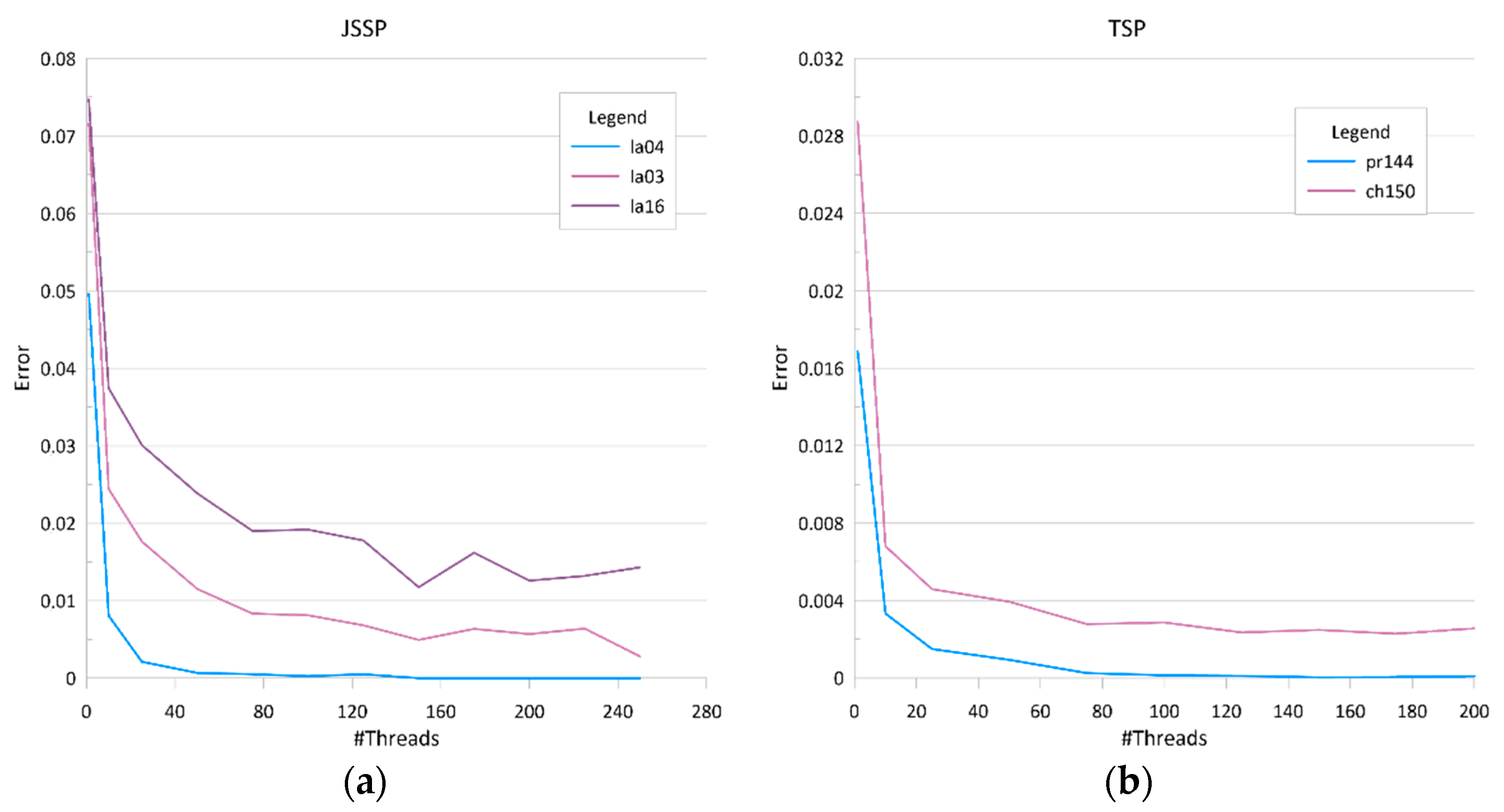
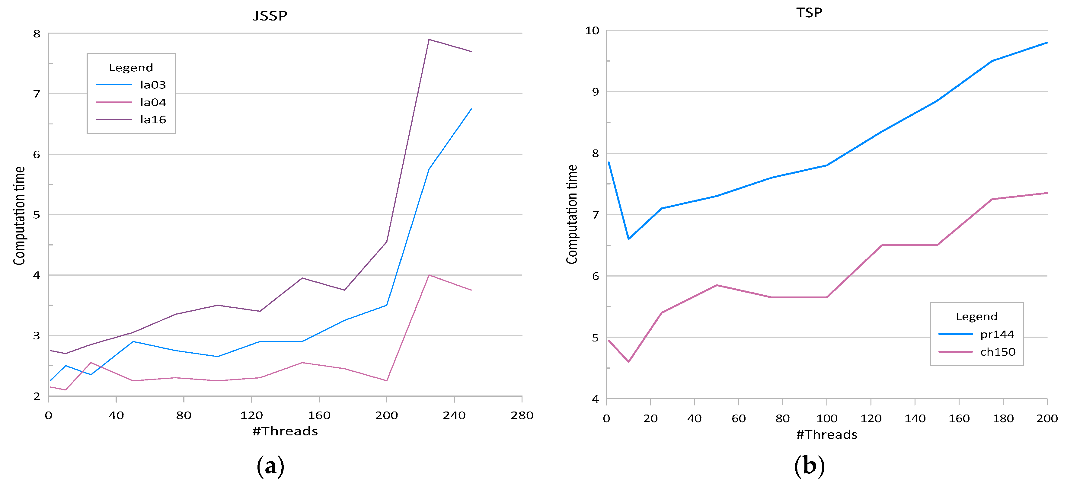
Further experiments were carried out to identify some properties of the convergence ability of the MPA. Figure 1 shows the dependency between the number of threads and mean accuracy for example benchmark datasets. Pr144 was solved with 4 solutions processed in each thread, the other datasets used 2 solutions in each thread. Computation results were averaged over 20 runs, searchTime was equal 0.5 seconds, stopping criterion was defined as no improvement in the best fitness for 2 rounds. Figure 2 shows dependency between the number of threads and mean computation times in the same experiment. It may be noticed that using more threads results in obtaining better solutions since more solutions from the search space are considered. However, increasing the number of threads also results in increasing the time required for communication. In addition, at some point, depending on the number of nodes in the cluster, some of the threads are executed sequentially.

3.3. MPA Performance versus other Approaches

Further experiments aimed at comparing the performance of the MPA with performance of other, state-of-the-art algorithms.

Table 5. Settings and results with standard deviations for the analyzed TSP datasets.

Dataset	Opt	SearchTime (s)	Err	Time (s)	SD err	SD Time (s)
kroA100	21,282	0.2	0.00%	2.50	0.00%	1.28
pr107	44,303	0.2	0.00%	6.40	0.00%	2.70
pr76	108,159	0.2	0.00%	2.33	0.00%	1.11
ch130	6110	0.5	0.00%	8.30	0.01%	2.31
eil101	629	0.5	0.00%	5.20	0.00%	1.40
pr124	59,011	0.5	0.03%	21.43	0.00%	10.43
pr144	58,537	0.5	0.00%	9.55	0.00%	1.50
a280	2579	1	0.16%	49.50	0.15%	11.36
bier127	118,282	1	0.03%	20.03	0.06%	4.72
ch150	6528	1	0.08%	12.70	0.13%	3.54
kroA150	26,524	1	0.01%	17.70	0.05%	5.49
kroA200	29,368	1	0.03%	27.27	0.05%	5.86
kroB100	22,086	1	0.27%	10.63	0.06%	3.26
kroB150	26,130	1	0.00%	15.73	0.00%	3.80
kroB200	29,438	1	0.00%	27.26	0.01%	5.20
pcb442	50,778	1	1.11%	622.28	0.41%	272.84
pr299	48,191	1	0.09%	102.47	0.09%	31.93
tsp225	3016	1	0.62%	37.95	0.40%	8.20
pr1002	259,045	5	2.34%	6549.76	0.32%	2636.14

presents results obtained for instances of the TSP for different values of the searchTime. Calculations were carried out using the set of agents consisting of bestMove, randomReverse and crossover. Computations were carried out using 175 threads. The stopping criterion was defined as no improvement in the best fitness for 5 rounds. In

Table 6. Comparison of the performance of the mushroom-picking algorithm (MPA) with other algorithms (TSP datasets).

	MPA		DSOS [21]		NDDE [19]		CII [27]
Dataset	Err (%)	Time (s)	Err	Time (s)	Err	Time (s)	Err	Time (ms)
kroA100	0.00%	2.50	0.60%	127.5	0.21%	2.8	0.80%	3.5
pr107	0.00%	6.40	0.32%	187.3	–	–	2.20%	18.1
pr76	0.00%	2.33	0.36%	–	–	–	4.40%	3.0
ch130	0.00%	8.30	–	–	–	–	1.30%	27.9
eil101	0.00%	5.20	3.43%	171.8	0.65%	3.5	5.90%	19.5
pr124	0.03%	21.43	0.68%	235.6	–	–	1.70%	5.3
pr144	0.00%	9.55	0.48%	516.6	0.02%	3.5	2.30%	6.8
a280	0.16%	49.50	–	–	–	–	4.10%	52.9
bier127	0.03%	20.03	–	–	–	–	2.80%	5.6
ch150	0.08%	12.70	0.38%	–	–	–	3.30%	11.5
kroA150	0.01%	17.70	–	–	–	–	2.70%	10.2
kroA200	0.03%	27.27	–	–	–	–	4.80%	17.5
kroB100	0.27%	10.63	0.90%	138.1	–	–	2.60%	3.3
kroB150	0.00%	15.73	–	–	–	–	1.00%	26.4
kroB200	0.00%	27.26	–	–	–	–	4.10%	11.8
pcb442	1.11%	622.28	–	–	0.72%	16.6	4.90%	126.0
pr299	0.09%	102.47	–	–	–	–	4.20%	43.6
tsp225	0.62%	37.95	–	–	–	–	6.80%	22.9
pr1002	2.34%	6549.76	7.46%	1843.3	–	–	6.60%	744.0

the results are compared with some other results known from the literature,

A comparison with [27] is especially interesting as in the CII very similar one-argument functions were applied to a single initial solution. CII is much faster (time is expressed in milliseconds in this case) than MPA. In return, our method outperforms CII in terms of the computation errors.

Table 7. Mean errors, computations times (s) and their standard deviations for the analyzed JSSP datasets.

Datasets	Opt	Err	Time (s)	SD Err	SD Time (s)
la01	666	0.00%	0.5	0.00%	1.0
la02	655	0.00%	1.3	0.00%	1.0
la03	597	0.84%	1.8	0.57%	1.4
la04	590	0.24%	1.2	0.42%	1.2
la05	593	0.00%	0.6	0.00%	0.9
la06	926	0.00%	0.6	0.00%	1.1
la07	980	0.00%	1.2	0.00%	1.1
la08	863	0.00%	0.6	0.00%	1.3
la09	951	0.00%	0.7	0.00%	1.1
la10	958	0.00%	0.6	0.00%	1.0
la11	1222	0.00%	0.8	0.00%	1.2
la12	1039	0.00%	0.7	0.00%	1.2
la13	1150	0.00%	0.6	0.00%	1.1
la14	1292	0.00%	0.7	0.00%	1.0
la15	1207	0.00%	30.53	0.00%	1.7
la16	945	0.31%	41.37	0.49%	9.3
la17	784	0.06%	39.54	0.14%	8.8
la18	848	0.20%	41.10	0.32%	8.9
la19	842	1.01%	42.09	0.59%	9.0
la20	901	0.50%	32.90	0.17%	4.7
la21	1046	3.03%	79.47	0.82%	15.0
la22	927	2.08%	74.67	0.66%	14.3
la23	1032	0.00%	45.00	0.00%	6.6
la24	935	3.50%	64.67	1.20%	12.3
la25	977	3.52%	77.63	1.14%	24.7
la26	1218	1.61%	105.97	1.01%	23.5
la27	1235	4.49%	120.50	0.93%	33.8
la28	1216	3.15%	113.70	1.00%	28.2
la29	1152	7.77%	120.67	1.16%	37.3
la30	1355	0.61%	112.00	0.75%	29.6
la31	1784	0.00%	64.37	0.00%	6.4
la32	1850	0.00%	85.33	0.00%	12.0
la33	1719	0.00%	73.57	0.00%	8.4
la34	1721	0.36%	172.47	0.50%	33.9
la35	1888	0.03%	95.20	0.15%	17.9
la36	1268	4.53%	79.67	1.10%	23.1
la37	1397	4.94%	94.00	1.06%	25.5
la38	1196	7.02%	106.03	1.31%	30.5
la39	1233	4.25%	99.47	1.49%	24.0
la40	1222	3.69%	109.00	1.06%	26.2

presents results obtained for instances of the JSSP. In this case the set of agents consisting of randomMove, randomReverse and crossover were used. searchTime of one round and stopping criterion was defined as 2 deciseconds and 2 rounds with no improvement in the best solution for la01 to la14, and 5 s and 5 rounds with no improvement for la15 to la49. In

Table 8. Comparison of MPA performance with other methods for the analyzed JSSP datasets.

Datasets	MPA		DWPA [33]		Naga [32]
	Err	Time (s)	Err	Time (s)	Err
la01	0.00%	0.5	0.00%	1.30	0.32%
la02	0.00%	1.3	0.00%	2.10	2.20%
la03	0.84%	1.8	2.85%	1.70	4.88%
la04	0.24%	1.2	1.36%	1.10	–
la05	0.00%	0.6	0.00%	1.30	–
la06	0.00%	0.6	0.00%	2.40	0.00%
la07	0.00%	1.2	0.00%	2.00	0.09%
la08	0.00%	0.6	0.00%	2.40	–
la09	0.00%	0.7	0.00%	2.40	–
la10	0.00%	0.6	0.00%	1.50	–
la11	0.00%	0.8	0.00%	3.80	0.00%
la12	0.00%	0.7	0.00%	1.70	0.00%
la13	0.00%	0.6	0.00%	3.90	–
la14	0.00%	0.7	0.00%	3.90	–
la15	0.00%	30.53	5.47%	3.40	–
la16	0.31%	41.37	5.08%	2.60	–
la17	0.06%	39.54	1.15%	2.30	–
la18	0.20%	41.10	1.53%	2.30	–
la19	1.01%	42.09	5.46%	3.40	–
la20	0.50%	32.90	3.55%	2.20	–
la21	3.03%	79.47	5.64%	7.30	2.06%
la22	2.08%	74.67	6.69%	6.20	–
la23	0.00%	45.00	1.84%	5.50	–
la24	3.50%	64.67	5.67%	5.60	–
la25	3.52%	77.63	6.35%	5.30	–
la26	1.61%	105.97	6.98%	6.00	1.53%
la27	4.49%	120.50	8.99%	9.40	–
la28	3.15%	113.70	6.17%	11.30	–
la29	7.77%	120.67	10.68%	12.4	–
la30	0.61%	112.00	2.51%	8.7	–
la31	0.00%	64.37	0.00%	17.1	12.24%
la32	0.00%	85.33	0.00%	18.5	–
la33	0.00%	73.57	0.00%	15.4	–
la34	0.36%	172.47	3.89%	14.5	–
la35	0.03%	95.20	3.13%	17.7	–
la36	4.53%	79.67	9.46%	9.9	–
la37	4.94%	94.00	6.37%	18.2	–
la38	7.02%	106.03	11.97%	11.5	–
la39	4.25%	99.47	8.19%	17.4	–
la40	3.69%	109.00	10.23%	10.0	–

the MPA results are compared with some other recently published results. Errors for [33] and [32] were computed on the base of results given in the respective papers. In [32] only mean errors were reported with no information on the computation time.

4. Discussion

The proposed mushroom-picking algorithm was validated using benchmark datasets from the TSP and JSSP publicly available repositories. The first of the reported experiments aimed at identifying the best combination of the available agents.

For the TSP, the best combination denoted BR consists of the bestMove and randomReverse agents plus the crossover. The BR, with mean error averaged over all considered dataset at the level of 0.28% was significantly better than RR, BB, RB with the respective mean errors of 0.36%, 0.41% and 0.45%. The above finding was confirmed by the Friedman ANOVA by ranks test at the significance level of 0.05. In the case of the TSP also differences between mean computation times have proven to be statistically significant. The BR not only provides the smallest mean error, but also assures the shortest mean computation time, which was again established by the Friedman ANOVA by ranks test at the significance level of 0.05.

For the JSSP, the best combination denoted RR consists of the randomMove and randomReverse agents plus the crossover. The RR, with the mean computation error averaged over all considered dataset at the level of 3.75% was significantly better than BR with the respective mean error of 11.53%. The above finding was confirmed by the Wilcoxon Signed Rank Test at the significance level of 0.05. However, comparison of the mean computation times by the same method have confirmed that there are no significant differences between mean computation times of RR and BB.

Another feature of the MPA is its stability. In the case of the TSP, the mean value of the standard deviation of the computation error, averaged over all considered datasets, is 0.18% with maximum deviation at 0.95% and minimum at 0.0%. In the case of the JSSP the respective values are 0.92% with maximum at 3.43% and minimum at 0.0%.

Convergence analysis in the case of both TSP and JSSP shows that increasing the number of threads rapidly decreases computation errors. The rule is valid up to certain number of threads. Further increasing of this number decreases computation errors in a much lower pace until a zero or stable error level was reached. Computation time analysis shows that up to a point where the stable computation error was reached, increasing the number of threads increases the computation time at a slow rate. The above dependency is clearly visible in the case of the JSSP as opposed to the case of the TSP where the growth of the computation time with the increase of the number of threads is nearly linear.

The performance of the MPA was compared with performances of the recently published algorithms for solving the TSP and JSSP. Data from Table 6 show that for the TSP, MPA outperforms other competing approaches including DSOS, NDDE and CII. Unfortunately, due to the high number of missing values for the DSOS and NDDE performance, we were not able to carry out a full statistical analysis of the compared results. The mean computation error in the case of the TSP, calculated over all sample datasets for the MPA is 0.25% while the same value for the CII algorithm is 3.5%. In return, the CII algorithm is much quicker with the mean computation time of 17.05 ms versus 22.17 s in the case of the MPA (both values calculated without pcb442 and pr1002 datasets). Data from Table 8 show that for JSSP our approach outperforms DWPA and NAGA. Unfortunately, due to the high number of missing values in the case of the NAGA we were not able to carry out the Friedman ANOVA by ranks test. The mean computation error in the case of the JSSP, calculated over all sample datasets for the MPA is 1.44% and 3.53% for the DWPA. DWPA offers, however, a shorter computation time with the average of 6.9 s versus 53.32 s for the MPA.

5. Conclusions

The study proposes an approach for solving the TSP and JSSP instances in which a swarm of agents tries to improve solutions from the population of solutions. The approach named mushroom-picking algorithm is a population-based metaheuristic implemented in the parallel computation environment. The proposed algorithm offered good or very good performance-producing solutions that were optimal or close to optimal, within in a reasonable time.

The performance of the MPA is encouraging from the point of view of the future research. One possible direction is extending the spectrum of a simple result improving agents. Some restrictions on the process of selecting results for improvement may result in decreasing computation time by eliminating unproductive attempts. It is also expected to implement the approach using different environments for parallel computing.

References

- Goldberg, D.E. Genetic Algorithms in Search, Optimization and Machine Learning, 1st ed.; Addison-Wesley Longman Publishing Co., Inc.: Boston, MA, USA, 1989. [Google Scholar]
- Fogel, D.B. Evolutionary Computation: Toward a New Philosophy of Machine Intelligence; IEEE Press: Piscataway, NJ, USA, 1995. [Google Scholar]
- Kennedy, J.; Eberhart, R. Particle Swarm Optimization. In Proceedings of the ICNN’95—International Conference on Neural Networks, Perth, WA, Australia, 27 November–1 December 1995; Volume 4, pp. 1942–1948. [Google Scholar] [CrossRef]
- Dorigo, M.; Maniezzo, V.; Colorni, A. Ant System: Optimization by a Colony of Cooperating Agents. IEEE Trans. Syst. Man Cybern. Part B (Cybern.) 1996, 26, 29–41. [Google Scholar] [CrossRef] [PubMed] [Green Version]
- Sato, T.; Hagiwara, M. Bee System: Finding solution by a concentrated search. In Proceedings of the 1997 IEEE International Conference on Systems, Man, and Cybernetics. Computational Cybernetics and Simulation, Orlando, FL, USA, 12–15 October 1997; Volume 4, pp. 3954–3959. [Google Scholar]
- Boussaï, I.; Lepagnot, J.; Siarry, P. A Survey on Optimization Metaheuristics. Inf. Sci. 2013, 237, 82–117. [Google Scholar] [CrossRef]
- Jedrzejowicz, P. Current Trends in the Population-Based Optimization. Computational Collective Intelligence; Nguyen, N.T., Chbeir, R., Exposito, E., Aniorté, P., Trawinski, B., Eds.; Springer International Publishing: Cham, Switzerland, 2019; pp. 523–534. [Google Scholar]
- Chu, X.; Wu, T.; Weir, J.; Shi, Y.; Niu, B.; Li, L. Learning–interaction–diversification framework for swarm intelligence optimizers: A unified perspective. Neural Comput. Appl. 2020, 32, 1789–1809. [Google Scholar] [CrossRef]
- Beni, G.; Wang, J. Swarm Intelligence in Cellular Robotic Systems. In Robots and Biological Systems: Towards a New Bionics; Dario, P., Sandini, G., Aebischer, P., Eds.; Springer: Berlin/Heidelberg, Germany, 1993; pp. 703–712. [Google Scholar]
- Freitas, D.; Lopes, L.; Morgado-Dias, F. Particle Swarm Optimisation: A Historical Review Up to the Current Developments. Entropy 2020, 22, 362. [Google Scholar] [CrossRef] [Green Version]
- Darwish, A.; Hassanien, A.E.; Das, S. A survey of swarm and evolutionary computing approaches for deep learning. Artif. Intell. Rev. 2019, 53, 1767–1812. [Google Scholar] [CrossRef]
- Peska, L.; Misikir Tashu, T.; Horvath, T. Swarm intelligence techniques in recommender systems—A review of recent research. Swarm Evol. Comput. 2019, 48. [Google Scholar] [CrossRef]
- Velusamy, B.; Pushpan, S.C. A Review on Swarm Intelligence Based Routing Approaches. Int. J. Eng. Technol. Innov. 2019, 9, 182–195. [Google Scholar]
- Zedadra, O.; Guerrieri, A.; Jouandeau, N.; Spezzano, G.; Seridi, H.; Fortino, G. Swarm intelligence-based algorithms within IoT-based systems: A review. J. Parallel Distrib. Comput. 2018, 122, 173–187. [Google Scholar] [CrossRef]
- Mahi, M.; Ömer, K.B.; Kodaz, H. A new hybrid method based on Particle Swarm Optimization, Ant Colony Optimization and 3-Opt algorithms for Traveling Salesman Problem. Appl. Soft Comput. 2015, 30, 484–490. [Google Scholar] [CrossRef]
- Gülcü, S.; Mahi, M.; Baykan, O.; Kodaz, H. A parallel cooperative hybrid method based on ant colony optimization and 3-Opt algorithm for solving traveling salesman problem. Soft Comput. 2016. [Google Scholar] [CrossRef]
- Osaba, E.; Yang, X.S.; Diaz, F.; Lopez-Garcia, P.; Carballedo, R. An improved discrete bat algorithm for symmetric and asymmetric Traveling Salesman Problems. Eng. Appl. Artif. Intell. 2016, 48, 59–71. [Google Scholar] [CrossRef]
- Gupta, I.K.; Shakil, S.; Shakil, S. A Hybrid GA-PSO Algorithm to Solve Traveling Salesman Problem. In Computational Intelligence: Theories, Applications and Future Directions—Volume I; Verma, N.K., Ghosh, A.K., Eds.; Springe: Singapore, 2019; pp. 453–462. [Google Scholar]
- Ali, I.M.; Essam, D.; Kasmarik, K. A novel design of differential evolution for solving discrete traveling salesman problems. Swarm Evol. Comput. 2020, 52, 100607. [Google Scholar] [CrossRef]
- Akhand, M.; Ayon, S.I.; Shahriyar, S.; Siddique, N.; Adeli, H. Discrete Spider Monkey Optimization for Travelling Salesman Problem. Appl. Soft Comput. 2020, 86, 105887. [Google Scholar] [CrossRef]
- Ezugwu, A.E.S.; Adewumi, A.O. Discrete symbiotic organisms search algorithm for travelling salesman problem. Expert Syst. Appl. 2017, 87, 70–78. [Google Scholar] [CrossRef]
- Paul, D.P.V.; Chandirasekaran, G.; Dhavachelvan, P.; Ramachandran, B. A novel ODV crossover operator-based genetic algorithms for traveling salesman problem. Soft Comput. 2020. [Google Scholar] [CrossRef]
- Er, H.R.; Erdogan, N. Parallel Genetic Algorithm to Solve Traveling Salesman Problem on MapReduce Framework using Hadoop Cluster. JSCSE 2014. [Google Scholar] [CrossRef]
- Alanzi, E.; Bennaceur, H. Hadoop MapReduce for Parallel Genetic Algorithm to Solve Traveling Salesman Problem. Int. J. Adv. Comput. Sci. Appl. 2019, 10. [Google Scholar] [CrossRef]
- Karouani, Y.; Elhoussaine, Z. Efficient Spark-Based Framework for Solving the Traveling Salesman Problem Using a Distributed Swarm Intelligence Method. In Proceedings of the 2018 International Conference on Intelligent Systems and Computer Vision (ISCV), Fez, Morocco, 2–4 April 2018. [Google Scholar] [CrossRef]
- Jedrzejowicz, P.; Wierzbowska, I. Apache Spark as a Tool for Parallel Population-Based Optimization. In Proceedings of the KES Conference on Intelligent Decision Technologies 2019, St. Julien’s, Malta, 17–19 June 2019; pp. 181–189. [Google Scholar]
- Pacheco-Valencia, V.; Hernández, J.A.; Sigarreta, J.M.; Vakhania, N. Simple Constructive, Insertion, and Improvement Heuristics Based on the Girding Polygon for the Euclidean Traveling Salesman Problem. Algorithms 2020, 13, 5. [Google Scholar] [CrossRef] [Green Version]
- Çalis, B.; Bulkan, S. A research survey: Review of AI solution strategies of job shop scheduling problem. J. Intell. Manuf. 2013, 26, 961–973. [Google Scholar] [CrossRef]
- Hu, H.; Lei, W.; Gao, X.; Zhang, Y. Job-Shop Scheduling Problem Based on Improved Cuckoo Search Algorithm. Int. J. Simul. Model. 2018, 17, 337–346. [Google Scholar] [CrossRef]
- Zhang, Z.; Guan, Z.; Zhang, J.; Xie, X. A Novel Job-Shop Scheduling Strategy Based on Particle Swarm Optimization and Neural Network. Int. J. Simul. Model. 2019, 18, 699–707. [Google Scholar] [CrossRef]
- Zhu, J.; Shao, Z.; Chen, C. An Improved Whale Optimization Algorithm for Job-Shop Scheduling Based on Quantum Computing. Int. J. Simul. Model. 2019, 18, 521–530. [Google Scholar] [CrossRef]
- Chen, X.; Zhang, B.; Gao, D. Algorithm Based on Improved Genetic Algorithm for Job Shop Scheduling Problem. In Proceedings of the 2019 IEEE International Conference on Mechatronics and Automation (ICMA), Tianjin, China, 4–7 August 2019. [Google Scholar] [CrossRef]
- Wang, F.; Tian, Y.; Wang, X. A Discrete Wolf Pack Algorithm for Job Shop Scheduling Problem. In Proceedings of the 2019 5th International Conference on Control, Automation and Robotics (ICCAR), Beijing, China, 19–22 April 2019. [Google Scholar] [CrossRef]
- Vital-Soto, A.; Azab, A.; Baki, M.F. Mathematical modeling and a hybridized bacterial foraging optimization algorithm for the flexible job-shop scheduling problem with sequencing flexibility. J. Manuf. Syst. 2020, 54, 74–93. [Google Scholar] [CrossRef]
- Anuar, N.I.; Fauadi, M.H.F.M.; Saptari, A. Performance Evaluation of Continuous and Discrete Particle Swarm Optimization in Job-Shop Scheduling Problems. Mater. Sci. Eng. Conf. Ser. 2019, 530, 012044. [Google Scholar] [CrossRef]
- Tsai, C.W.; Chang, H.C.; Hu, K.C.; Chiang, M.C. Parallel coral reef algorithm for solving JSP on Spark. In Proceedings of the 2016 IEEE International Conference on Systems, Man, and Cybernetics (SMC), Budapest, Hungary, 9–12 October 2016. [Google Scholar] [CrossRef]
- Sun, L.; Lin, L.; Lib, H.; Gen, M. Large Scale Flexible Scheduling Optimization by A Distributed Evolutionary Algorithm. Comput. Ind. Eng. 2018, 128. [Google Scholar] [CrossRef]
- Jędrzejowicz, P.; Ratajczak-Ropel, E. PLA Based Strategy for Solving RCPSP by a Team of Agents. J. Univers. Comput. Sci. 2016, 22, 856–873. [Google Scholar]
- Barbucha, D.; Czarnowski, I.; Jedrzejowicz, P.; Ratajczak-Ropel, E.; Wierzbowska, I. Team of A-Teams—A Study of the Cooperation between Program Agents Solving Difficult Optimization Problems. In Agent-Based Optimization; Czarnowski, I., Jedrzejowicz, P., Kacprzyk, J., Eds.; Springer: Berlin/Heidelberg, Germany, 2013; pp. 123–141. [Google Scholar] [CrossRef]
- Apache Spark. Available online: https://spark.apache.org/ (accessed on 14 January 2019).
- Source Files of MPA for TSP. Available online: https://bitbucket.org/wierzbowska/mpa-for-tsp/src/master/ (accessed on 21 May 2020).
- Reinelt, G. TSPLIB. Available online: http://www.iwr.uni-heidelberg.de/groups/comopt/software/TSPLIB95/ (accessed on 14 January 2019).
- Lawrence, S. Resource Constrained Project Scheduling-Technical Report; Carnegie-Mellon University: Pittsburgh, PA, USA, 1984. [Google Scholar]
Figure 1.
Mean error versus the number of threads for some example (a) traveling salesman (TSP) and (b) job-shop scheduling (JSSP) datasets.
Figure 2.
Mean computation time (s) versus the number of threads for some example (a) TSP and (b) JSSP datasets.