Efficient Probabilistic Joint Inversion of Direct Current Resistivity and Small-Loop Electromagnetic Data


1
Department of Environment, Ghent University, Coupure Links 653, 9000 Gent, Belgium
2
Department of Geology, Ghent University, 9000 Gent, Belgium
*
Author to whom correspondence should be addressed.
Algorithms 2020, 13(6), 144; https://0-doi-org.brum.beds.ac.uk/10.3390/a13060144
Submission received: 27 March 2020
/
Revised: 7 June 2020
/
Accepted: 13 June 2020
/
Published: 18 June 2020
Abstract
:Often, multiple geophysical measurements are sensitive to the same subsurface parameters. In this case, joint inversions are mostly preferred over two (or more) separate inversions of the geophysical data sets due to the expected reduction of the non-uniqueness in the joint inverse solution. This reduction can be quantified using Bayesian inversions. However, standard Markov chain Monte Carlo (MCMC) approaches are computationally expensive for most geophysical inverse problems. We present the Kalman ensemble generator (KEG) method as an efficient alternative to the standard MCMC inversion approaches. As proof of concept, we provide two synthetic studies of joint inversion of frequency domain electromagnetic (FDEM) and direct current (DC) resistivity data for a parameter model with vertical variation in electrical conductivity. For both studies, joint results show a considerable improvement for the joint framework over the separate inversions. This improvement consists of (1) an uncertainty reduction in the posterior probability density function and (2) an ensemble mean that is closer to the synthetic true electrical conductivities. Finally, we apply the KEG joint inversion to FDEM and DC resistivity field data. Joint field data inversions improve in the same way seen for the synthetic studies.
1. Introduction
In applied geophysics, subsurface images are derived from non-invasive geophysical measurements, for example, direct current (DC) resistivity or small-loop electromagnetic (EM) measurements at the earth’s surface. Geophysical data acquired from such measurements can be translated into a subsurface image of the investigated physical property by inversion of the data. Geological units often differ in terms of their physical properties; for example, ore bodies can usually be distinguished from their surroundings by identifying the spatial distribution of electrical conductivities in the subsurface. For this reason, inverse images can be useful to geologists, for example, in identifying mineral and hydrocarbon resources, groundwater reservoirs, and geological structures.
Geophysical inverse problems are almost always ill-posed, i.e., no unique solution to the problem can be calculated [1]. This ill-posedness arises from the following general problems that are attributed to geophysical data collection: an inherent non-uniqueness (mostly problematic using potential methods), inaccuracies in data collection, possible inconsistencies in the data set, and, most importantly, an insufficient amount of data. Even for data sets acquired in the most precise manner (no noise or systematic errors), only limited information about the subsurface can be inferred, usually being insufficient for resolving the non-uniqueness of the inverse problem.
One approach for improving geophysical inverse images is the so-called joint inversion of multiple geophysical data sets of different measurement responses [2]. Joint inversion usually refers to a simultaneous inversion of two or more data sets for a common subsurface parameter model. In general, joint inversions can be carried out for data sets informing two or more different sets of model parameters by using some kind of defined relation between the different types of parameters. However, joint inversions for methods that are sensitive to different subsurface properties will not be considered in this manuscript.
Because different types of data contain complementary information about the subsurface, it is expected that the non-uniqueness of the inverse problem is mitigated (but not resolved) when data are inverted jointly. For the type of measurement data discussed in this paper, DC electrical resistivity and EM data, several approaches for joint inversion were presented in the literature (for example, by [3,4,5,6]). In particular, Sharma and Kaikkonen [5] summarize the use of joint in version of the two data types: EM inversion alone is useful for resolving thin conductive layers, but fails for detecting thin resistive layers in conductive surroundings. DC resistivity data on the other hand suffer from a general equivalence problem when resolving the thickness versus conductivity/resistivity ratio of a thin layer [7]. The joint inversions presented in the publications listed above applied deterministic gradient-based geophysical inversion approaches [8]. These studies showed the beneficial properties of joint inversions over the application of multiple separate inversions, for example the successful detection of thin middle layers was only achieved in joint results [4].
Two main problems are associated with the application of deterministic approaches in joint inversion frameworks. First, deterministic inversions have no measure for the theoretically expected reduction of uncertainty when applying joint inversion. The only available measure is the data misfit, which can generally be similar for different inversion approaches and, therefore, does not provide an objective assessment of the improvement brought by joint inversion. A model misfit computation is only available for synthetic studies and thus, unavailable for field data studies. Second, deterministic inversion schemes require largely arbitrary weights in the objective function, expressing the influence of the different data types on the objective function and the role of the regularization functional (e.g., [9]).
Bayesian inference is one way to quantify the non-uniqueness or uncertainty of an inverse problem. Moreover, Bayesian inversion approaches are readily available to be used as a joint inversion framework and they do not require weighing the different data types. Additionally, errors other than noise can be included in the processing, for example, using hierarchical or empirical Bayesian approaches [10]. However, we do not consider hierarchical or empirical Bayesian frameworks for the work presented in this manuscript, as we expect a relatively small influence of additional errors.
For typical geophysical problems, i.e., non-linear and large dimensional problems, no analytical solution for Bayes’ theorem can be given, which makes the numerical sampling of probability density functions (PDFs) necessary. The standard approach in geophysics is the Markov chain Monte Carlo (MCMC) method applying Metropolis- or Gibbs-sampling [1]. This approach is well-known to converge to the exact posterior PDF for a infinite runtime of the algorithm approaching infinity. Highly-parametrized models result in computationally expensive forward model runs that limit the applicability of MCMC methods [11]. Only recently, efficient approximations of the posterior distribution have been proposed for geophysical problems, while using innovative methods, such as the Kalman ensemble generator (KEG, [12]) or Bayesian Evidential Learning [13]. Those techniques rely on a smaller number of forward model runs and are, thus, less expensive. Unfortunately, highly-parametrized models are often indispensable in order to model complex geological structures beyond horizontal stratigraphy. Ultimately, a convergence of the chain computations of MCMC might not be achievable within the number of affordable forward model runs, which is why MCMC approaches are rarely seen in geophysical literature on fully non-linear joint inversion.
In this work, we apply the Kalman ensemble generator (KEG, [14]) as an efficient alternative to a MCMC inversion framework to solve the joint inverse problem. The KEG is a stationary implementation of the ensemble Kalman filter [15] and, thus, a Monte Carlo implementation of a probabilistic least-squares formulation [1]. If the Gaussian assumption is applicable to all parameters, it was shown that the ensemble Kalman filter can be applied to non-linear forward models. In contrast to MCMC approaches, we do not need the chain approach and conduct independent random sampling instead. Therefore, there is no burn-in phase and no rejection of proposed samples. Thus, in the KEG framework, all Monte Carlo samples can directly be used to characterize a Gaussian approximation to the posterior PDF.
The objective of this paper is to apply the KEG for joint probabilistic inversion of DC resistivity and small-loop EM data. previously applied to the inversion of EM [12], yet, to the best of our knowledge, this is the first time that (1) the method is used for geophysical joint inversion and (2) that these types of data are jointly inverted in a probabilistic way. We present two examples of simulated geophysical measurements for synthetic one-dimensional subsurface models and one field data example showing vertical contrasts in electrical conductivity. This way, we investigate whether the expected uncertainty reduction of the inverse image using two types of data simultaneously can be assessed and resolved by the approximate Gaussian solution to the Bayesian update problem. For this purpose, we will compare KEG posterior PDFs of the separate inversions of DC resistivity data and of EM data with the joint KEG inversion result. Additionally, we investigate whether the posterior ensemble mean gives an improved image for the subsurface, i.e., if it is shifted closer to the true synthetic model of subsurface electrical conductivity. For one synthetic example, we investigate the influence of sample size on the posterior estimates.
The remainder of this manuscript is structured as follows. First, we explain the particular forward models used to simulate geophysical measurement data. In particular, we use a DC resistivity Schlumberger vertical electrical sounding configuration and a small-loop frequency-domain EM forward model. Second, we outline the (joint) KEG approach in the context of Bayesian inference. Subsequently, we demonstrate the application of the KEG for synthetic examples. Using separate and joint KEG inversions, we compare their performance for estimating the same one-dimensional subsurface model of electrical conductivity. In total, we provide two synthetic studies for KEG joint inversions: (1) a four-layer model with fixed layer boundaries functioning as a toy model for a concise visualization of the results and (2) a more application-oriented inversion for a synthetic subsurface model with many discrete model layers. For the latter, we analyze the influence of the sample size on the results. Finally, the KEG approach is used for separate and joint multi-layer inversion of EM and DC resistivity field data.
2. Methodology
In this section, we describe the tools that are required to perform a joint inversion of direct current (DC) resistivity and small-loop electromagnetic (EM) data. In particular, these include (1) the two forward models used for describing the relation between electrical conductivity (EC) and DC resistivity and EM data and (2) the inversion method used, in this case the Kalman ensemble generator (KEG).
2.1. Frequency-Domain Electromagnetics
Several different measurement configurations for EM data exist, and all of them are sensitive to the EC of the subsurface. The EM method that is discussed in this work is the small loop-loop frequency-domain electromagnetic (FDEM) induction method [16]. Applying small-loop FDEM techniques, a primary electromagnetic field is generated by an alternating current of a single low frequency, in our case 9 kHz, in a transmitter coil that is approximated by a magnetic dipole [17]. The resulting EM field propagation can be described by a diffusion equation. This field induces eddy currents in conductive material that is affected by the primary field. These eddy currents generate a secondary field. The secondary field, together with the primary field, is recorded at one or multiple receiver coils placed at a defined distance from the transmitter coil. Besides the transmitter-receiver offset, the measurement sensitivity depends largely on the respective coil geometries (see Figure 1b). The strength of the secondary field can be related to the subsurface EC, the measurement quantity of interest. The secondary field is usually expressed as in-phase (IP) and quadrature-phase (QP) components in relation to the primary field [16], below expressed in parts-per-million [ppm].
In this work, we simulate FDEM data using the code that was provided by Hanssens et al. (2019) [18], applying the physical equations, as given by Ward and Hohmann (1988) [17]. Their description, using a one-dimensional full solution of Maxwell’s equations, denotes a non-linear relation between the measurement and electrical conductivity of the subsurface volume affected by the induction phenomena.
It is well-known that small loop-loop FDEM field data are prone to severe systematic errors [19]. Thus, for the field data application described at the end of our text, we modify the FDEM forward model by adding a simple offset term to the QP and IP responses [20]. These offsets denote the possible systematic errors that are included in the IP and QP responses.
2.2. Vertical Electrical Sounding
Direct current resistivity data are usually collected using a four-point electrode-configuration at the earth’s surface. Such a configuration consists of one pair of current electrodes, injecting a defined current into the ground, and a second pair of electrodes recording the resulting voltage. In this work, we will employ the Schlumberger setup for vertical electrical sounding (VES), as this is often applied for the exploration of vertical variation of EC and, thus, often used in one-dimensional EC modeling of the subsurface [21]. For Schlumberger VES measurements, the pair of voltage electrode stays fixed in line with the current electrodes, whereby the distance between the current electrodes is increased after each voltage measurement. Using Ohm’s law and assuming a homogeneous half-space for the entire subsurface, the recorded voltage can be expressed as apparent electrical conductivity (EC). The apparent EC can be linked to the spatial distribution of the subsurface electrical conductivity distribution. A thorough description of the VES forward model used can be found in Everett [22].
2.3. Bayesian Inference and the Kalman Ensemble Generator
In Bayesian inversion approaches, all of the available information is translated into a probability distribution. Bayesian updates modify prior information by relevant measurement data producing posterior probability distributions for model parameters.
The prior information is given as a probability density function (PDF) for the model parameters . Inserting into the relevant geophysical forward model g, and combining with the observations , we derive the likelihood function , the probability for a set of observations given the parameters. Here, and denote the number of parameters and number of observations, respectively. Bayes’ theorem defines the posterior probability density function in terms of the PDFs discussed above:
where random variables left of a vertical bar are conditional to a set of values for the random variables on the right side of the bar and denotes a normalization factor.
In joint inversions, consists of data of two different types of geophysical measurements. Assuming that the measurement errors between the two data sets are uncorrelated, Blatter et al. [23] point out that the likelihood in a joint Bayesian framework can simply be given as the product of the individual likelihoods:
with a joint data vector
for VES data and FDEM data .
Dealing with high-dimensional non-linear problems, no analytical solution is available to solve Equation (1). Instead, the posterior needs to be numerically sampled. Most commonly, this is done using Markov chain-Monte Carlo (MCMC) methods applying a Metropolis- or Gibbs-sampler. Using an infinite number of samples, this approach converges to the exact solution of the Bayesian update problem [24]. However, in practice, the computational resources are limited and the applicability of MCMC methods is therefore restricted. Computational restrictions are particularly pressing when expensive forward models are necessary and large data sets are used, which is usually the case in geophysical applications. Often, an MCMC sampler is no longer feasible for computing solutions to such problems as no convergence of the chain can be achieved within the number of affordable forward model runs.
Here, we will apply a specific Monte Carlo implementation of the Bayesian update problem: the ensemble Kalman filter (EnKf, [15]). The EnKf was introduced as an efficient alternative to the original Kalman filter [25] for solving large-dimensional and non-linear problems in data assimilation [26]. In the EnKf context, the set of Monte Carlo samples is called an ensemble. The ensemble formulation makes the EnKF more efficient than the Kalman filter for two reasons: (1) in contrast to the the Kalman filter, the covariance equation can be replace by sample covariance and (2) Jacobian computations are unnecessary avoiding many calls of the forward model.
Instead of the Jacobian, the full forward response g is computed for all ensemble realizations:
where is the size of the ensemble, is the measurement error, and and are realisations of the Gaussian prior PDF and Gaussian data PDF, respectively. The ensemble is generated by drawing multivariate normal random numbers from the multivariate Gaussian prior using the Matlab function ‘mvnrnd’ [27].
The EnKf update equation is given by [15]:
for . The covariances , and are derived from the prior ensemble given by matrix and the forward response ensemble given by matrix , where is the number of observations and is the number of model parameters. Correcting the matrices and for their respective mean values, those are named and , and can be used for covariance computation, as follows:
where is derived from the matrix of ensemble means
where corresponds to the matrix with each element equal to [15]. The mean-corrected matrix is computed according to
Matrix is computed analogously to matrix .
In the context of stationary inversion theory, the ensemble Kalman filter is called Kalman ensemble generator (KEG, [14]). In contrast to the MCMC samplers, the KEG does not use a Markov chain to explore the model parameter space. Instead, the KEG requires that the Gaussian assumption is applicable to all PDFs [28]. Likewise, the posterior PDF derived from the KEG update is considered a Gaussian; therefore, it can be understood as a Gaussian approximation to the true (non-Gaussian) posterior PDF.
In contrast, MCMC approaches converge to the exact posterior solution for near-exhaustive sampling. However, in MCMC computations, consecutive samples in the chain are correlated, causing lower efficiency than KEG for the following reasons. First, the early Monte Carlo samples might be biased and must be skipped; this corresponds to the so-called burn-in phase [8]. Second, due to the requirement of independent random samples in statistical analysis, only every n-th sample can be used to characterize the posterior PDF. Third, the acceptance rate of samples (using the mostly used Metropolis sampler) is between 30 and 50% [1]. Finally, the chain computations cannot be parallelized. In contrast, the KEG is built on independent random sampling without the need of rejection sampling and, consequently, each sample can (1) be used for the characterization of the posterior PDF and (2) be run fully in parallel.
The KEG was only recently adopted for the inversion of geophysical data. Bobe et al. [12] applied it to the inversion of frequency-domain electromagnetic data to the probabilistic estimation of electrical conductivity and magnetic susceptibility. As for other probabilistic methods, a joint framework is readily available while using the KEG. In such frameworks, no weighing of different data types is necessary as long as significant errors in the parameter estimation are limited to Gaussian noise. Instead, the covariances available from Monte Carlo sampling determining the relative weight of each measurement. This holds for all types of measurement, irrelevant of the fact of whether the data are EM or DC resistivity data.
The likelihood is generated by passing on all prior realizations in to both forward models and . Thus, for the same EC realizations of the subsurface, signals for both measurement techniques are computed. Those responses are summarized in a forward response ensemble matrix
An efficient implementation of the KEG is given by [14]:
This matrix equation summarizes the computations described in Equation (5), where matrix is the ensemble data matrix, with uncorrelated Gaussian noise, defining a Gaussian PDF that ultimately defines the overall diagonal data covariance matrix . The mean corrected version of matrix is named .
Matrix is characterized by its mean value, being considered as the best fit to the measurement data, and a standard deviation (STD) as corresponding uncertainty around the best fit. For a more detailed description of this inversion approach applied in a geophysical context see [12].
Restricting the posterior estimate to its Gaussian approximation has computational advantages over MCMC processing. Gaussian PDFs can be sampled directly and the samples are truly random, such that (1) no model rejection or burn-in phase is necessary [24] and (2) forward computations can be performed in parallel.
3. Synthetic Cases
We present two synthetic inversions to demonstrate a probabilistic joint inversion using the KEG. For both cases, we compare the results for the joint inversions with the results for the separate inversions of DC resistivity and FDEM data.
The first test case is a simple toy model chosen primarily for a simplified visualization of the parameter estimates. The simplification consists in limiting the inversion to four parameters, in particular, the electrical conductivity of four subsurface layers with fixed layer boundaries.
The second synthetic test case shows the results of a multi-layer inversion, which means that, for this case, the number of discrete layers, i.e., inversion parameters, is chosen much larger than the expected number of subsurface layers. Thus, the exact number of subsurface layers does not need to be defined a priori.
For the inversion of VES and FDEM data, we define the model parameters of logarithmic electrical conductivity. The logarithmic barrier prevents unphysical updates, i.e., negative estimates of electrical conductivity.
For both cases, we simulate observations for the true synthetic model using the same forward model that is used in the inversion process. Thus, errors that arise from imperfect forward models are neglected in this study. The ensemble of the prior model and forward responses are identical, thus errors that arise from sampling bias are identical for all of the separate and joint inversion results.
3.1. Four-Layer Inversion
In a first synthetic toy case, we simulate FDEM and VES data for a subsurface that consists of four layers with contrast in electrical conductivity. The synthetic true model is shown in Figure 1a.
The VES data is simulated for an electrode spacing of 30 cm for the voltage electrodes and 30 cm for the current electrodes (compare Figure 1c). The FDEM data is simulated for one transmitter coil and four distinct receiver coils, two in horizontal co-planar (HCP) configuration in 1 and 2 m distance from the transmitter, and two in perpendicular (PRP) configuration in 1.1 and 2.1 m distance from the transmitter coil (compare Figure 1b). The simulated forward responses for the synthetic true model are listed in Figure 1b,c. Small Gaussian white noise of 0.1% was added to all simulated measurements and, as such, considered for the construction of the measurement ensemble .
We consider a uniform Gaussian prior model, i.e., the same Gaussian PDF for all model parameters, to exclude further spurious correlation from the inverse processing. Additionally, we define a simple diagonal covariance matrix for the prior model parameters. For the construction of the prior PDF, mean and standard deviation of the logarithmic electrical conductivity of the synthetic true model are considered in steps of 10 cm. Using this mean and STD, we construct the same Gaussian prior PDF for all four model parameters. In particular, the prior mean is set to 0.0581 S/m, with the prior ranging within one STD to the upper limit of 0.1195 S/m and the lower limit of 0.0282 S/m. The Gaussian prior PDFs are sampled to construct the ensemble matrix , and is used to compute the forward response ensemble matrix (Equation (9)).
The results for the separate and joint inversion of VES and FDEM data are given in the covariance matrix-like plot in Figure 2 [8]. The posterior estimates of the four model parameters are given on the diagonal of the figure. Additionally, the ensemble mean estimates, i.e., the best fits, together with the synthetic true model, are shown in the lower left part of Figure 2. On the off-diagonals, we show scatter plots of pairs of estimated model parameters.
The point clouds in the scatter plots on the off-diagonals in Figure 2 illustrate the range of parameter estimates that are compatible with the measurement data. Some interesting aspects are linked to the shapes of these point clouds. First, the point clouds have different shapes and locations for the three applied inversions. This implies that the two data sets do include mutually different information regarding the subsurface. Second, the point clouds for FDEM inversion are smaller than the ones for VES inversion. This is in accordance with the expectations for low-noise FDEM data, as signal generation is limited to distinct flows of the induced eddy currents, making the FDEM data, in theory, less prone to non-uniqueness. Third, the range compatible with both data sets is smaller than the range compatible with both separate data sets. This complies with the expectation that a joint inversion approach reduces parameter uncertainty.
The parameter estimates that are shown on the diagonal in Figure 2 allow further conclusions regarding the performance of the joint inversion. First, all posterior solutions enclose the synthetic true solution. Second, for all four model parameter estimates, the joint posterior PDF shows the smallest STD. This is in accordance with the expectations for joint inversions of different data, since a decrease in STD illustrates the reduction of uncertainty in the inversion result. Third, the ensemble mean estimate for the inversion of the joint data set is, in all cases, closest to the EC of the synthetic true model. Most noticeable for the posterior estimates of the EC of layer two and three, the joint result is not a simple average or mean of the separate inversion results.
Overall, the results outlined above point to the fact that the KEG can provide the expected benefits that are associated with joint inversion of two types of geophysical data sets over the separate inversions of the latter.
3.2. Multi-Layer Inversion
As a more application-oriented example of a joint inversion using the KEG, in which the number and thickness of subsurface layers do not need to be known a priori, we introduce a parameter model with a large number of discrete model layers. In this example, the synthetic true model consists of three distinct subsurface layers showing vertical contrast in EC (dotted line in Figure 3): an upper layer of 70 cm thickness and an EC of 0.2 S/m, a resistive (0.08 S/m) intermediate layer of 1 m, and a bottom layer extending to infinite depth with an EC of 0.1 S/m. The amount of discrete layers is chosen so large that it is expected that the boundaries of the discrete layers will not strongly influence the Bayesian update. The discrete model layers are 10 cm thick. We use an ensemble of size 10,000 to sample the defined PDFs.
Similar to the procedure for the few-layer inversion, we derive logarithmic mean and STD for the EC of all discrete model layers. Mean and STD define the prior Gaussian PDF for all of the model parameters. Again, no correlation between prior model parameters is implemented. This way, we aim to derive a Gaussian prior model uniform in depth, imposing as little spurious correlation as possible on the inversion procedure. This prior selection results in a mean of 0.1054 S/m with the prior ranging within one STD to the upper limit of 0.1388 S/m and the lower limit of 0.0800 S/m.
The measurement setups used for simulation of VES and FDEM data equal the ones that were used for the previous few-layer inversion example. In particular, the VES data is simulated for a voltage electrode offset of 30 cm, the current electrodes add another 30 cm for the first measurement. Thereafter, the current electrode offset is extended in 30 cm steps, up to a total extent of 15 m. The FDEM data are simulated for four receiver coils with offsets and geometrical configurations, as shown in Figure 1. Gaussian noise of 0.1% is added to this simulated measurement values and thereafter used for construction of matrix .
In Figure 3, the results for separate and joint KEG inversions are compared to the synthetic true model. Overall, the joint parameter estimate shows the smallest uncertainty around the best fit models. For almost all posterior model parameters, the true synthetic model is included within two STDs around this ensemble mean. Exceptions can be found around the upper layer boundary. The large EC contrast at the layer boundaries is not always captured within two STDs due to the smoothing effect of the multi-layer inversion.
The different best fit models, i.e., the ensemble means, can be compared to the synthetic true model for their ability to characterize layers of different EC. In general, the best fit of the FDEM data inversion give good estimates for the uppermost layer. In contrast, the VES data inversion better characterizes the EC of the lowermost layer. However, while the top layer is distinctly represented in all three inversion results, for the separate VES and FDEM inversions, intermediate and bottom layer cannot clearly be distinguished by analysis of the best fit models. In contrast, in the best fit model derived from joint inversion, there is a clear difference of the average EC estimate for intermediate and bottom layer. The quality of the fits derived from the separate and joint inversions are quantified computing the root-mean-square error (RMSE) between the synthetic true models and the ensemble mean estimates. The results for the RMSEs are given in Table 1. As expected from visual comparison in Figure 3, the best fit for the joint inversion gives a smaller RMSE than the separate inversions of VES and FDEM data.
To provide insight on the efficiency of the joint KEG method, we investigate the above example for different ensemble sizes. We compare the KEG results for an ensemble of size 100, 1000, 2500, 10,000, and 100,000.
The best fits for the synthetic study with different sample size are shown in Figure 4. For this example, the small ensemble sizes, 100 and 1000, lead to strong fluctuations that hinder a straightforward interpretation of the best fit functions. As expected, it shows that a larger ensemble leads to smaller fluctuations around the synthetic true.
We first correct the best fit for the synthetic true model by subtracting the respective true conductivity value from the best fit functions, in logarithmic domain, in order to quantify the reduction in fluctuation. For discrete layers that cover a subsurface layer boundary, we subtract a weighted mean based on the share of of the discrete layer above and below the layer boundary. This computation results in an approximately Gaussian distribution around zero for all model parameters. The root mean square (RMS) of these distributions might serve as a measure for the sampling error introduced by small ensemble sizes (Table 2).
In general, the STD becomes smaller with an increasing sample size. However, the decrease of the STD is steeper for the comparison of small absolute ensemble size. In contrast, the STD-decrease between 10,000 and 100,000 ensemble members is minor. Likewise, this minor difference reflects in the similarity of the best fit functions in Figure 4. Therefore, it is possible to derive a threshold value above which an increase in the sample size does not yield a significant improvement in the posterior estimate. This threshold is likely dependent on the data type and the model complexity. However, the threshold might be approximated using synthetic benchmarking, as presented here. A similar observation has been made for other approximate Bayesian methods (e.g., [13]).
4. Field Data Case
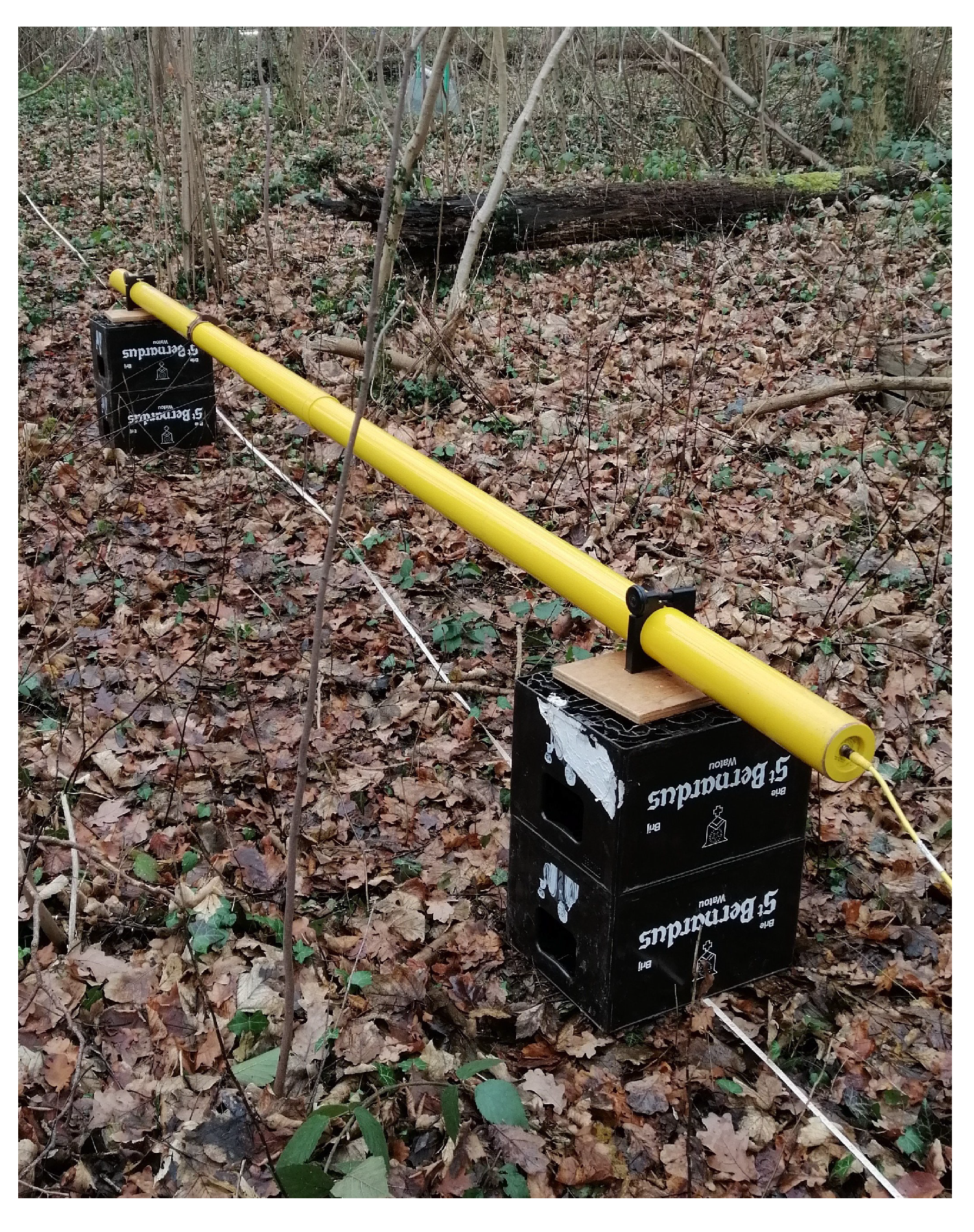
In order to demonstrate the joint KEG inversion for geophysical field data, we apply it to a FDEM and a VES data set acquired for estimating a vertical soil EC profile for a forest soil in Gontrode, Belgium. The exact measurement location was selected for its horizontal stratigraphy of different soil layers conformed to the one-dimensional (1D) assumption. The VES and FDEM data sets were recorded at the same day to minimize the possible effects of varying conditions in soil water saturation. In particular, the VES data set was collected by the commercial resistivity meter four-point light 10 W (LGM Lippmann, Schaufling, Germany) while using electrode spacings of one meter, with a total profile length of 14 m. FDEM data were collected in the center of the VES profile, with a setup of six receiver coils. This FDEM setup is similar to the one that is shown in Figure 1b, with an additional set of HCP and PRP coils at 4 and 4.1 m, respectively, a DUALEM-421S (Dualem Inc., Milton, ON, Canada). For calibration purposes [20], the FDEM data were collected with the same instrument at two heights: ground level and 0.6 m above ground (see Figure 5).
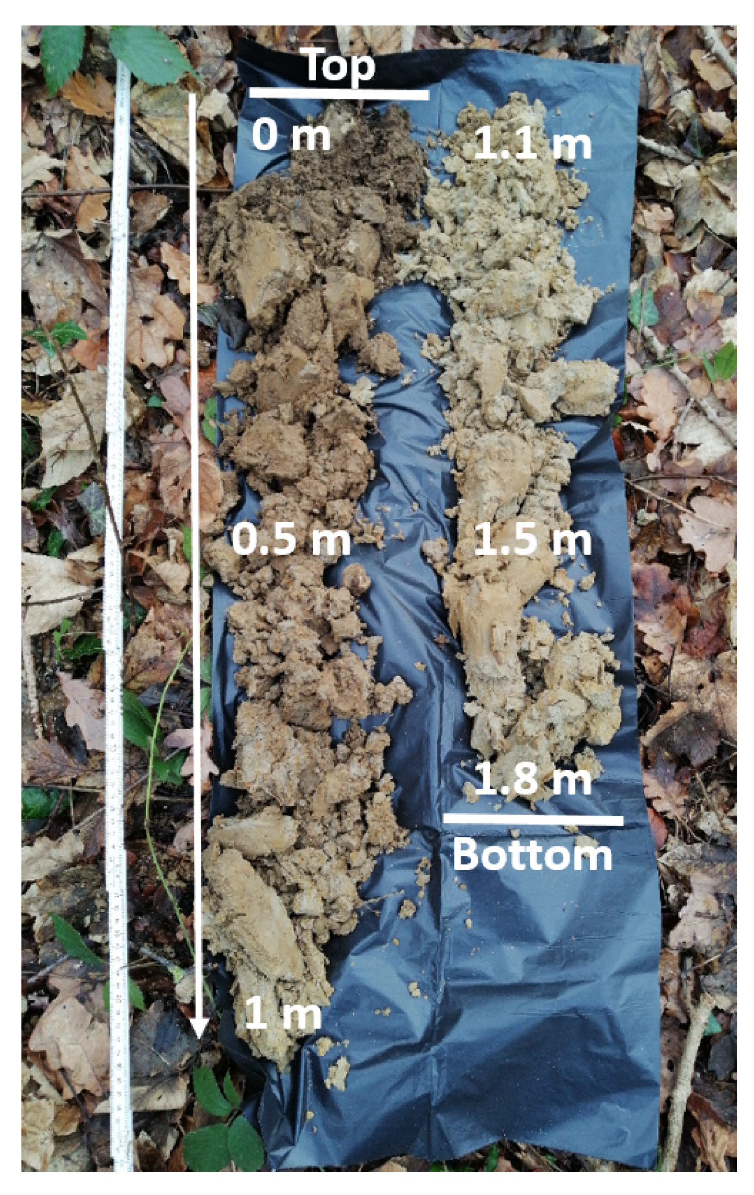
For the validation of the EC profile, a vertical hole was drilled using an Edelmann auger. Figure 6 shows the drilling output. From the drilling output, multiple soil layers were visually distinguished. For the top 0.15 m, we found an organic rich forest material (plants and other organic material), including several air-filled voids. Below 0.15 m down to approximately 0.8 m, a clay-rich sand was found. Below 0.8 m, the clay content decreased with increasing depth, which resulted in a relatively higher sand content. Around 1.5 m, the groundwater table was reached.
To link a possible inversion result to the above soil profile description, we explain some general relations of the present subsurface material and its influence on the bulk EC [29]. First, air is known as an insulator, thus, significant shares of air-filled voids will result in a relatively low bulk EC value. High clay content is known to result in relatively high conductivities as compared to the average soil due to surface charges on the mineral surface. In contrast, sand is known for its relatively low EC values, therefore, an increase in sand content is expected to lower the bulk EC of the soil. The presence of groundwater usually coincides with an increase in EC, due to the presence of free electrical charge carriers.
For inverse modeling, we used an approach similar to the one described for the synthetic multi-layer inversion. First, a prior model was defined for discrete horizontal model layers of 8.5 cm thickness. The prior model mean was chosen to cover a large EC range expected from auger drilling. In particular, the prior model mean is 0.02 S/m with one STD ranging to an upper limit of 0.04 S/m and a lower limit of 0.01 S/m. Twelve offset parameters were added to the prior model for the calibration of the FDEM data: two offsets for each IP and QP signal of each receiver coil [20]. The prior offsets are a priori unknown and, therefore, a prior PDF with mean of zero and a relatively large STD of 100 ppm was defined (corresponding to an average of 9.3% of the magnitude of the measurement values). For the two types of data, different noise levels were estimated from repeated VES and FDEM measurements. These noise levels were used for defining the PDFs that provide the basis for the construction of data matrix . We chose an ensemble size of 50,000 for this study based on the results of the synthetic sample size study and the fine discretization chosen for this study. The total computation time (on the same personal computer) for the separate VES inversion was 53.06 s, and for the separate FDEM inversion 724.36 s. The total computation time of the joint inversion was 770.49 s using the same prior and and forward response ensemble. The difference in the update step computation time between VES/FDEM inversion and the joint inversion was 0.07 and 0.15 s, respectively.
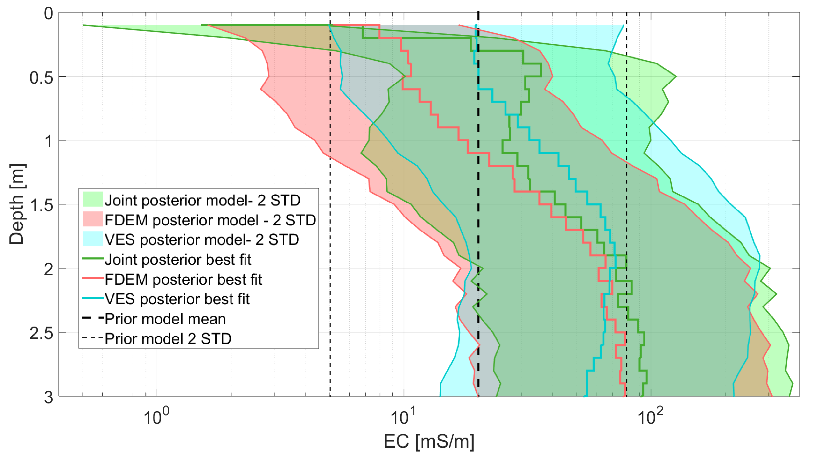
In Figure 7, we show the results for separate and joint KEG inversion of VES and FDEM data. All of the profiles result in EC estimates in the same order of magnitude. The best fit models of both separate inversion both approximately indicate an increase of EC with depth. However, in the best fit from joint inversion, a different soil EC profile is derived. First, the top is estimated as relatively resistive, followed by a distinct increase of soil EC up to a depth of approximately 0.5 m. Below 0.5 m, the EC value decreases again down to a depth of 1 m. For the lower most part of the profile below 1 m, the EC is increasing again.
Although smooth results of multi-layer inversion are difficult to interpret in terms of distinct soil or ground water layers, the joint best fit EC profile is in better agreement with the soil profile from auger drilling. Especially, the increase in clay content for the profile section between 0.15 m and 0.7 m agrees with the higher EC in the best fit joint profile. In both best fit profiles from separate inversion, this section of increased EC cannot be observed.
Besides the difference in shape of the best fit profiles, the magnitude of uncertainty can be compared for the three posterior models. Whereas the profiles from the separate inversions only show a small reduction of the prior uncertainty for the upper, most sensitive, profile parameters, the joint posterior model results in a comparably larger reduction of uncertainty. With increasing depth, i.e., with a decrease in measurement sensitivity, the uncertainty magnitude increases until, finally, the joint STD is in the same order of magnitude as for the other posterior models. Overall, the supposed properties of the joint posterior model, as described in the previous two paragraphs, are in agreement with the expectations for joint inversion as compared to the separate inversions.
5. Conclusions
We used the Kalman ensemble generator (KEG) as a framework for performing geophysical joint inversion. Joint inversion was performed for two synthetic data sets and one field data set, each consisting of direct current (DC) resistivity and frequency-domain electromagnetic (FDEM) data. When compared to the results of separate KEG inversion of VES and FDEM data, joint inversion resulted in better estimations with smaller uncertainty.
Like most probabilistic inversions, the KEG is readily extendable into a joint inversion framework, without the need for specific input for weighing the influence of each considered data set. It should be noted though that the KEG is a much more efficient solver for the non-linear joint inversion than the commonly applied probabilistic methods, i.e., Markov chain Monte Carlo (MCMC) approaches. This efficiency is achieved by restricting all probability density function to Gaussianity. On the one hand, this means that the KEG only yields a Gaussian approximation to the posterior PDF. On the other hand, the KEG works without rejection sampling and a burn-in phase. Thus, each sample can be used for the direct characterization of the posterior. Additionally, the joint KEG inversion is fully parallelizable, especially concerning the most computationally expensive step, the computation of the forward problems for the two (or more) types of geophysical methods.
Joint KEG inversion of DC resistivity and FDEM yielded two major benefits over separate KEG inversions, namely (1) a reduction of uncertainty in the joint posterior model and (2) a best fit model that is closer to the true subsurface parameter variation. This is illustrated by the reduction of the range of estimated model parameters using the joint framework. Additionally, in our study, the estimated joint parameter range is not a simple mean or average of the range estimated in the corresponding separate inversions. The joint inversion resolved distinct features that were not resolved by both separate inversion results providing that an ensemble size is used that is large enough to sufficiently suppress spurious correlation. In the investigated synthetic example, a sample size of 10,000 was sufficient as adding more samples did not significantly improve the posterior estimates computed.
The KEG application to the VES and FDEM field data set shows that the joint processing of both data sets is straightforward in a real world setting. Here, the only difference between synthetic and field data processing consists in the additional offset parameters added to the simulation of FDEM forward responses, mediating the often encountered severe systematic errors in FDEM field data. The joint KEG inversion resulted in an EC profile that was well in accordance with the soil profile derived by auger drilling. Additionally, like for the synthetic data case, but less pronounced, the posterior uncertainty derived from joint inversion is smaller than the uncertainty derived from separate inversions.
Overall, the KEG is a functional tool for joint probabilistic inversion. In the future, the limitations of the method, in particular the Gaussian assumption and possibility of normal-score transform for non-Gaussian prior models should be further investigated. Due to the computational advantages of the KEG over MCMC methods, we believe that the KEG has great potential for inverse modelling of complex two- and three-dimensional subsurface structures. Moreover, the KEG might be used for modeling of highly-parametrized problems as for such the KEG might not only outperform MCMC methods but also most gradient-based inversion methods that rely on many calls of the forward model.
Author Contributions
For this research article, the authors have contributed in the following way: C.B. proposed and implemented the main idea of the joint inversion, carried out the field work, processed the geophysical data, and wrote large sections of the manuscript. D.H. implemented the VES forward model. T.H. and E.V.D.V. contributed to the writing of this manuscript and supervised the project. All authors have read and agreed to the published version of the manuscript.
Funding
This project has received funding from the European Union’s EU Framework Programme for Research and Innovation Horizon 2020 under Grant Agreement No 721185.
Acknowledgments
The authors thank Valentijn Van Parys for his help with the field work.
Conflicts of Interest
The authors declare no conflict of interest.
References
- Tarantola, A. Inverse Problem Theory and Methods for Model Parameter Estimation; SIAM: Philadelphia, PA, USA, 2005. [Google Scholar]
- Moorkamp, M. Integrating electromagnetic data with other geophysical observations for enhanced imaging of the earth: A tutorial and review. Surv. Geophys. 2017, 38, 935–962. [Google Scholar] [CrossRef] [Green Version]
- Gomez-Trevino, E.; Edwards, R. Electromagnetic soundings in the sedimentary basin of southern Ontario—A case history. Geophysics 1983, 48, 311–330. [Google Scholar] [CrossRef]
- Raiche, A.; Jupp, D.; Rutter, H.; Vozoff, K. The joint use of coincident loop transient electromagnetic and Schlumberger sounding to resolve layered structures. Geophysics 1985, 50, 1618–1627. [Google Scholar] [CrossRef]
- Sharma, S.; Kaikkonen, P. Appraisal of equivalence and suppression problems in 1D EM and DC measurements using global optimization and joint inversion. Geophys. Prospect. 2003, 47, 219–249. [Google Scholar] [CrossRef]
- Yi, M.J.; Sasaki, Y. 2-D and 3-D joint inversion of loop–loop electromagnetic and electrical data for resistivity and magnetic susceptibility. Geophys. J. Int. 2015, 203, 1085–1095. [Google Scholar] [CrossRef] [Green Version]
- Koefoed, O. Geosounding Principles, 1. Resistivity Sounding Measurements; Elsevier Science Publishing Co.: Amsterdam, The Netherlands, 1979. [Google Scholar]
- Aster, R.C.; Borchers, B.; Thurber, C.H. Parameter Estimation and Inverse Problems; Elsevier: Amsterdam, The Netherlands, 2018. [Google Scholar]
- Commer, M.; Newman, G.A. Three-dimensional controlled-source electromagnetic and magnetotelluric joint inversion. Geophys. J. Int. 2009, 178, 1305–1316. [Google Scholar] [CrossRef] [Green Version]
- Malinverno, A.; Briggs, V.A. Expanded uncertainty quantification in inverse problems: Hierarchical Bayes and empirical Bayes. Geophysics 2004, 69, 1005–1016. [Google Scholar] [CrossRef]
- Sambridge, M.; Mosegaard, K. Monte Carlo methods in geophysical inverse problems. Rev. Geophys. 2002, 40, 3-1–3-29. [Google Scholar] [CrossRef] [Green Version]
- Bobe, C.; Van De Vijver, E.; Keller, J.; Hanssens, D.; Van Merivenne, M.; De Smedt, P. Probabilistic 1-D inversion of frequency-domain electromagentic data using a Kalman ensemble generator. IEEE Trans. Geosci. Remote Sens. 2019, 58, 3287–3297. [Google Scholar] [CrossRef]
- Michel, H.; Nguyen, F.; Kremer, T.; Elen, A.; Hermans, T. 1D geological imaging of the subsurface from geophysical data with Baeysian Evidential Learning. Comput. Geosci. 2020, 138, 104456. [Google Scholar] [CrossRef]
- Nowak, W. Best unbiased ensemble linearization and the quasi-linear Kalman ensemble generator. Water Resour. Res. 2009, 45. [Google Scholar] [CrossRef] [Green Version]
- Evensen, G. The ensemble Kalman filter: Theoretical formulation and practical implementation. Ocean Dyn. 2003, 53, 343–367. [Google Scholar] [CrossRef]
- Reynolds, J.M. An Introduction to Applied and Environmental Geophysics; John Wiley & Sons: Hoboken, NJ, USA, 2011. [Google Scholar]
- Ward, S.H.; Hohmann, G.W. Electromagnetic theory for geophysical applications. Electromagn. Methods Appl. Geophys. 1988, 1, 131–311. [Google Scholar]
- Hanssens, D.; Delefortrie, S.; De Pue, J.; Van Meirvenne, M.; De Smedt, P. Frequency-Domain Electromagnetic Forward and Sensitivity Modeling: Practical Aspects of Modeling a Magnetic Dipole in a Multilayered Half-Space. IEEE Geosci. Remote Sens. Mag. 2019, 7, 74–85. [Google Scholar] [CrossRef]
- Sasaki, Y.; Son, J.S.; Kim, C.; Kim, J.H. Resistivity and offset error estimations for the small-loop electromagnetic method. Geophysics 2008, 73, F91–F95. [Google Scholar] [CrossRef]
- Bobe, C.; Van De Vijver, E. Offset errors in probabilistic inversion of small-loop frequency-domain electromagnetic data: A synthetic study on their influence on magnetic susceptibility estimation. In Proceedings of the International Workshop on Gravity, Electrical & Magnetic Methods and Their Applications, Xi’an, China, 19–22 May 2019; Society of Exploration Geophysicists: Tulsa, OK, USA, 2019; pp. 312–315. [Google Scholar]
- Binley, A.; Kemna, A. DC resistivity and induced polarization methods. In Hydrogeophysics; Springer: Dordrecht, Switzerland, 2005; pp. 129–156. [Google Scholar]
- Everett, M.E. Near-Surface Applied Geophysics; Cambridge University Press: Cambridge, UK, 2013. [Google Scholar]
- Blatter, D.; Key, K.; Ray, A.; Gustafson, C.; Evans, R. Bayesian joint inversion of controlled source electromagnetic and magnetotelluric data to image freshwater aquifer offshore New Jersey. Geophys. J. Int. 2019, 218, 1822–1837. [Google Scholar] [CrossRef] [Green Version]
- Gelman, A.; Stern, H.S.; Carlin, J.B.; Dunson, D.B.; Vehtari, A.; Rubin, D.B. Bayesian Data Analysis; Chapman and Hall/CRC: London, UK, 2013. [Google Scholar]
- Kalman, R.E. A new approach to linear filtering and prediction problems. J. Basic Eng. 1960, 82, 35–45. [Google Scholar] [CrossRef] [Green Version]
- Burgers, G.; Jan van Leeuwen, P.; Evensen, G. Analysis scheme in the ensemble Kalman filter. Mon. Weather Rev. 1998, 126, 1719–1724. [Google Scholar] [CrossRef]
- MATLAB. MATLAB and Statistics Toolbox Release; The MathWorks Inc.: Natick, MA, USA, 2012. [Google Scholar]
- Zhou, H.; Gomez-Hernandez, J.J.; Franssen, H.J.H.; Li, L. An approach to handling non-Gaussianity of parameters and state variables in ensemble Kalman filtering. Adv. Water Resour. 2011, 34, 844–864. [Google Scholar] [CrossRef] [Green Version]
- Cassidy, N.J. Electrical and magnetic properties of rocks, soils and fluids. In Ground Penetrating Radar: Theory and Applications; Jol, H., Ed.; Elsevier: Amsterdam, The Netherlands, 2009; Volume 2, Chapter 2; pp. 41–72. [Google Scholar]
Figure 1.
(a) Synthetic true model consisting of four subsurface layers with the lowermost layer extending to infinite depth; and, corresponding simulated data for the synthetic subsurface model (b) simulated in-phase (IP) and quadrature (QP) response a for frequency-domain electromagnetic device in the setups, as shown, and (c) apparent electrical conductivity simulated for a vertical electrical sounding setup with current electrode spacing AB and a voltage electrode spacing both of 30 cm.

Figure 2.
Covariance matrix-like arrangement of scatter plots of the 1000 KEG samples of all parameter pairs from the posterior models for separate (blue and green) and joint (red) inversion of FDEM and VES data, including a larger black dot for the synthetic true solution. The four plots on the diagonal show the respective Gaussian posterior probability functions. The true subsurface model is shown in the lower left corner (black solid line) with its layer boundaries (black dashed line) being accompanied by the best fit (posterior mean) estimates derived from the respective separate and joint inversions.

Figure 3.
Kalman ensemble generator (KEG) inversion results for the same synthetic true model using the same prior model for vertical electrical sounding (VES) data, frequency domain electromagnetic (FDEM) data, and joint inversion of VES and FDEM data.
Figure 3.
Kalman ensemble generator (KEG) inversion results for the same synthetic true model using the same prior model for vertical electrical sounding (VES) data, frequency domain electromagnetic (FDEM) data, and joint inversion of VES and FDEM data.

Figure 4.
Best fit functions of joint Kalman ensemble generator (KEG) inversion results of FDEM and DC resistivity data for the same synthetic true model using the different sample sizes (SS) for ensemble creation, EC-axis in logarithmic scale.
Figure 4.
Best fit functions of joint Kalman ensemble generator (KEG) inversion results of FDEM and DC resistivity data for the same synthetic true model using the different sample sizes (SS) for ensemble creation, EC-axis in logarithmic scale.

Figure 5.
Multi-receiver FDEM measurement using a multi-receiver instrument at 0.6 m height; transmitter and receiver coils are arranged as sketched in Figure 1 with an additional HCP/PRP coil pair at 4 m/4.1 m, respectively.
Figure 5.
Multi-receiver FDEM measurement using a multi-receiver instrument at 0.6 m height; transmitter and receiver coils are arranged as sketched in Figure 1 with an additional HCP/PRP coil pair at 4 m/4.1 m, respectively.

Figure 6.
Output from auger drilling arranged according to approximate depth in the subsurface.

Figure 7.
Kalman ensemble generator (KEG) inversion results for the same synthetic true model using the same prior model for vertical electrical sounding (VES) data, frequency domain electromagnetic (FDEM) data, and joint inversion of VES and FDEM data.
Figure 7.
Kalman ensemble generator (KEG) inversion results for the same synthetic true model using the same prior model for vertical electrical sounding (VES) data, frequency domain electromagnetic (FDEM) data, and joint inversion of VES and FDEM data.


Table 1.
Comparison of root-mean-square errors (RMSEs) between the synthetic true model and the three best fit models (ensemble means) for separate and joint inversion of VES and FDEM data.
Table 1.
Comparison of root-mean-square errors (RMSEs) between the synthetic true model and the three best fit models (ensemble means) for separate and joint inversion of VES and FDEM data.
| VES | FDEM | Joint | |
|---|---|---|---|
| RMSE [mS/m] | 18.32 | 15.05 | 11.89 |
Table 2.
Root mean square (RMS) values for the best fit functions (corrected for synthetic true) computed for different sample size (SS) in the joint inversion.
Table 2.
Root mean square (RMS) values for the best fit functions (corrected for synthetic true) computed for different sample size (SS) in the joint inversion.
| SS | RMS |
|---|---|
| 100 | 0.201 |
| 1000 | 0.086 |
| 2500 | 0.081 |
| 10,000 | 0.069 |
| 100,000 | 0.067 |
© 2020 by the authors. Licensee MDPI, Basel, Switzerland. This article is an open access article distributed under the terms and conditions of the Creative Commons Attribution (CC BY) license (http://creativecommons.org/licenses/by/4.0/).
Share and Cite
MDPI and ACS Style
Bobe, C.; Hanssens, D.; Hermans, T.; Van De Vijver, E. Efficient Probabilistic Joint Inversion of Direct Current Resistivity and Small-Loop Electromagnetic Data. Algorithms 2020, 13, 144. https://0-doi-org.brum.beds.ac.uk/10.3390/a13060144
AMA Style
Bobe C, Hanssens D, Hermans T, Van De Vijver E. Efficient Probabilistic Joint Inversion of Direct Current Resistivity and Small-Loop Electromagnetic Data. Algorithms. 2020; 13(6):144. https://0-doi-org.brum.beds.ac.uk/10.3390/a13060144
Chicago/Turabian StyleBobe, Christin, Daan Hanssens, Thomas Hermans, and Ellen Van De Vijver. 2020. "Efficient Probabilistic Joint Inversion of Direct Current Resistivity and Small-Loop Electromagnetic Data" Algorithms 13, no. 6: 144. https://0-doi-org.brum.beds.ac.uk/10.3390/a13060144
Note that from the first issue of 2016, this journal uses article numbers instead of page numbers. See further details here.