On Multidimensional Congestion Games †


1
Department of Mathematics and Physics “Ennio De Giorgi”, University of Salento-Provinciale Lecce-Arnesano, P.O. Box 193, 73100 Lecce, Italy
2
Gran Sasso Science Institute-Viale Francesco Crispi 7, 67100 L’Aquila, Italy
3
Department of Information Engineering Computer Science and Mathematics, University of L’Aquila-Via Vetoio, Loc. Coppito, 67100 L’Aquila, Italy
*
Authors to whom correspondence should be addressed.
†
This work widely improves on an extended abstract presented at SIROCCO 2012.
Algorithms 2020, 13(10), 261; https://0-doi-org.brum.beds.ac.uk/10.3390/a13100261
Submission received: 9 September 2020
/
Revised: 27 September 2020
/
Accepted: 3 October 2020
/
Published: 15 October 2020
(This article belongs to the Special Issue Graph Algorithms and Applications)
Abstract
:We introduce multidimensional congestion games, that is, congestion games whose set of players is partitioned into clusters . Players in have full information about all the other participants in the game, while players in , for any , have full information only about the members of and are unaware of all the others. This model has at least two interesting applications: it is a special case of graphical congestion games induced by an undirected social knowledge graph with independence number equal to d, and it represents scenarios in which players have a type and the level of competition they experience on a resource depends on their type and on the types of the other players using it. We focus on the case in which the cost function associated with each resource is affine and bound the price of anarchy and stability as a function of d with respect to two meaningful social cost functions and for both weighted and unweighted players. We also provide refined bounds for the special case of in presence of unweighted players.
1. Introduction
Congestion games [1,2,3,4] are, perhaps, the most famous class of non-cooperative games due to their capability to model several interesting competitive scenarios, while maintaining nice properties. In these games, there is a set of players sharing a set of resources. Each resource has an associate cost function which depends on the number of players using it (the so-called congestion). Players aim at choosing subsets of resources so as to minimize the sum of the resource costs.
Congestion games were introduced by Rosenthal in Reference [2]. He proved that each such a game admits a bounded potential function whose set of local minima coincides with the set of pure Nash equilibria [5] of the game, that is, strategy profiles in which no player can decrease her cost by unilaterally changing her strategic choice. This existence result makes congestion games particularly appealing especially in all those applications in which pure Nash equilibria are elected as the ideal solution concept.
In these contexts, the study of inefficiency due to selfish and non-cooperative behavior has affirmed as a fervent research direction. To this aim, the notions of price of anarchy [6] and price of stability [7] are widely adopted. The price of anarchy (resp. stability) compares the performance of the worst (resp. best) pure Nash equilibrium with that of an optimal cooperative solution.
Congestion games with unrestricted cost functions are general enough to model the Prisoner’s Dilemma game, whose unique pure Nash equilibrium is known to perform arbitrarily bad with respect to the solution in which all players cooperate. Hence, in order to deal with significative bounds on the prices of anarchy and stability, some kind of regularity needs to be imposed on the cost functions associated with the resources. To this aim, lot of research attention has been devoted to the case of polynomial cost functions [8,9,10,11,12,13,14,15,16,17], and more general latency functions verifying some mild assumptions [10,18,19]. Among these, the particular case of affine functions occupies a predominant role. In fact, as shown in References [20,21,22], they represent the only case, together with that (perhaps not particularly meaningful) of exponential cost functions, for which weighted congestion games [20], that is the generalization of congestion games in which each player has a weight and the congestion of a resource becomes the sum of the weights of its users, still admit a potential function.
1.1. Motivations
Traditional (weighted) congestion games are defined under a full information scenario—each player knows all the other participants in the game as well as their available strategies. These requirements, anyway, become too strong in many practical applications, where players may be unaware about even the mere existence of other potential competitors. This observation, together with the widespread of competitive applications in social networks, has drawn some attention on the model of graphical (weighted) congestion games [23,24,25].
A graphical (weighted) congestion game is obtained by coupling a traditional (weighted) congestion game with a social knowledge graphG expressing the social context in which the players operate. In G, each node is associated with a player of and there exists a directed edge from node i to node j if and only if player i has full information about player j. A basic property of (weighted) congestion games is that the congestion of a resource r in a given strategy profile is the same for all players. The existence of a social context in graphical (weighted) congestion games, instead, makes the congestion of each resource player dependent. In these games, in fact, the congestion presumed by player i on resource r in the strategy profile is obtained by excluding from the set of players choosing r in those of whom player i has no knowledge. Clearly, if G is complete, then there is no difference between and . In all the other cases, however, there may be a big difference between the cost that a player presumes to pay on a certain strategy profile and the real cost that she effectively perceives because of the presence of players she was unaware of during her decisional process (We observe that the model of graphical congestion games is sufficiently powerful to describe an alternative scenario in which players never perceive their real costs, which are perceived and evaluated by a central entity only. In such case, the central entity aims at evaluating the global and real impact on the performance of the game caused by the players’ strategic behaviour).
Graphical congestion games have been introduced by Bilò et al. in Reference [24]. They focus on affine cost functions and provide a complete characterization of the cases in which existence of pure Nash equilibria can be guaranteed. In particular, they show that equilibria always exist if and only if G is either undirected or directed acyclic. Then, for all these cases, they give bounds on the price of anarchy and stability expressed as a function of the number of players in the game and of the maximum degree of G. These metrics are defined with respect to both the sum of the perceived costs and the sum of the presumed ones.
Fotakis et al. [25] argue that the maximum degree of G is not a proper measure of the level of social ignorance in a graphical congestion game and propose to bound the prices of anarchy and stability as a function of the independence number of G, denoted by . They focus on graphical weighted congestion games with affine cost functions and show that they still admit a potential function when G is undirected. Then, they prove that the price of anarchy is between and with respect to both the sum of the perceived costs and the sum of the presumed ones, and that the price of stability is between and with respect to the sum of the perceived costs.
1.2. Our Contribution and Significance
The works of Bilò et al. [24] and Fotakis et al. [25] aim at characterizing the impact of social ignorance in the most general case, that is, without imposing any particular structure on the social knowledge graphs defining the graphical game. Nevertheless, real-world-based knowledge relationships usually obey some regularities and present recurrent patterns: for instance, people tend to cluster themselves into well-structured collaborative groups (cliques) due to family memberships, mutual friendships, interest sharing, business partnerships.
To this aim, we introduce and study multidimensional (weighted) congestion games, that is, (weighted) congestion games whose set of players are partitioned into clusters . Players in have full information about all the other participants in the game, while players in , for any , have full information only about the members of and are unaware of all the others. It is not difficult to see (and we provide a formal proof of this fact in the next section) that each multidimensional (weighted) congestion game is a graphical (weighted) congestion game whose social knowledge graph G is undirected and verifies . In addition, G possesses the following, well-structured, topology: it is the union of disjoint cliques (each corresponding to one of the clusters in the multidimensional (weighted) congestion game) with the additional property that there exists an edge from all the nodes belonging to one of these cliques (the one corresponding to cluster ) to all the nodes in all the other cliques.
We believe that the study of graphical games restricted to some prescribed social knowledge graphs like the ones we consider here, may be better suited to understand the impact of social ignorance in non-cooperative systems coming from practical and real-world applications. Moreover, the particular social knowledge relationships embedded in the definition of multidimensional (weighted) congestion games perfectly model the situation that generates when several independent games with full information are gathered together by some promoting parties so as to form a sort of “global super-game”. The promoting parties become players with full information in the super-game, while each player in the composing sub-games maintains full information about all the other players in the same sub-game, acquires full information about all the promoting parties in the super game, but completely ignores the players in the other sub-games. Such a composing scheme resembles, in a sense, the general architecture of the Internet, viewed as a self-emerged network resulting from the aggregation of several autonomous systems (AS). Users in an AS have full information about anything happening within the AS, but, at the same time, they completely ignore the network global architecture and how it develops outside their own AS, except for the existence of high-level network routers. High-level network routers, instead, have full information about the entire network.
Furthermore, multidimensional (weighted) congestion games are also useful to model games in which players belong to different types and the level of competition that each player experiences on each selected resource depends on her type and on the types of the other players using the resource. Consider, for instance, a machine which is able to perform d different types of activities in parallel and a set of tasks requiring the use of this machine. Tasks are of two types: simple and complex. Simple tasks take the machine busy on one particular activity only, while complex tasks require the completion of all the d activities. Hence, complex tasks compete with all the other tasks, while simple ones compete only with the tasks requiring the same machine (thus, also with complex tasks). A similar example is represented by a facility location game where players want to locate their facilities so as to minimize the effect of the competition due to the presence of neighbor competitors. If we assume that the facilities can be either specialized shops selling particular products (such as perfumeries, clothes shops, shoe shops) or shopping centers selling all kinds of products, we have again that the shopping centers compete with all the other participants in the game, while specialized shops compete only with shops of the same type and with shopping centers.
In this paper, we focus on multidimensional (weighted) congestion games with affine cost functions. In such a setting, we bound the price of anarchy and the price of stability with respect to the two social cost functions, which are the sum of the perceived costs and the sum of the presumed costs. In fact, when multidimensional (weighted) congestion games are viewed as graphical (weighted) congestion games with highly clustered knowledge relationships, the sum of the perceived costs is more appropriate to define the overall quality of a profile: players decide according to their knowledge, but then, when the solution is physically realized, their cost becomes influenced also by the players of which they were not aware. Hence, under this social cost function, the notions of price of anarchy and price of stability effectively measure the impact of social ignorance in the system. On the other hand, when multidimensional (weighted) congestion games are used to model players belonging to different types, the perceived cost of a player coincides with the presumed one since there is no real social ignorance, even if the fact that players can be of different types allows for a reinterpretation of the model as a special case of graphical (weighted) congestion games. Hence, in such a setting, the inefficiency due to selfish behavior has to be analyzed with respect to the sum of the presumed costs.
We determine general upper bounds for the price of anarchy and the price of stability as a function of d. For the sum of the presumed costs, we show that the price of anarchy and stability of weighted games are at most and 2, respectively. Instead, for the sum of the perceived costs, the results of Reference [25] yield upper bounds of and for the price of anarchy and the price of stability, respectively.
Then, we investigate the case of unweighted games with (i.e., bidimensional congestion games) in higher depth and provide refined bounds. In particular, we prove that price of anarchy is with respect to the sum of the presumed costs and it is with respect to the sum of the perceived ones, and that the price of stability is between and for the sum of the presumed costs as social cost function, and between and for the sum of the perceived ones. These results are derived by exploiting the primal-dual method developed in Reference [11].
A preliminary version of this paper has been presented at SIROCCO 2012 [26].
1.3. Paper Organization
Next section contains all formal definitions and notation. In Section 3 we discuss the existence of pure Nash equilibria in multidimensional weighted congestion games. In Section 4 and Section 5, we present our bounds for the price of anarchy and the price of stability, respectively. Finally, in the last section, we give some concluding remarks and discuss open problems.
2. Model and Definitions
For an integer , we denote . In a weighted congestion game , we have n players and a set of resources R, where each resource has an associated cost function . The set of strategies for each player , denoted as , can be any subset of the powerset of R, that is, . Each player is associated with a positive weight . Given a strategy profile , the congestion of resource r in , denoted as , is the total weight of players choosing r in , that is, . The perceived cost paid by player i in is . An unweighted congestion game (congestion game, for brevity) is a weighted congestion game in which all players have unitary weights. An affine weighted congestion game is a weighted congestion game such that, for any , it holds that , with ; the game is linear if for any .
For any integer , a d-dimensional weighted congestion game consists of a weighted congestion game whose set of players is partitioned into clusters . For a player i, we denote by the cluster she belongs to. We say that players in are omniscient and that players in , for any , are ignorant. Given a strategy profile , we denote by the total weight of players belonging to who are using resource r in . The presumed cost of a player i in is if she is ignorant and if she is omniscient. A d-dimensional weighted affine congestion game is a pair such that is an affine weighted congestion game.
Given a strategy profile and a strategy for a player , we denote with the strategy profile obtained from by replacing the strategy played by i in with s. A pure Nash equilibrium is a strategy profile such that, for any player and for any strategy , it holds that .
Let be the set of all possible strategy profiles which can be realized in . We denote with the set of pure Nash equilibria of . Let be a social cost function measuring the overall quality of each strategy profile in . We denote with a social optimum of with respect to , that is, a strategy profile minimizing the social cost function . We consider two social cost functions, namely, the (weighted) sum of the presumed costs of all players and the (weighted) sum of their perceived ones denoted, respectively, as and . Technically, they assume the following expressions:
and
For a fixed social cost function , the price of anarchy of , denoted by , is the ratio between the social value of the worst pure Nash equilibrium of and that of a social optimum, that is, . The price of stability, denoted by , considers the best case, so that .
3. Existence of Pure Nash Equilibria
In this section, we prove that multidimensional unweighted (resp. weighted affine) congestion games are graphical unweighted (resp. weighted affine) congestion games defined by an underlying undirected social knowledge graph. This allows us to use a result in Reference [24] (resp. [25]) stating that these games are potential games, thus admitting pure Nash equilibria.
A graphical weighted congestion game consists of a weighted congestion game and a directed graph such that each node of N is associated with a player in and there exists a directed edge from node i to node j if and only if player i has full information about player j. The congestion presumed by player i on resource r in the profile is and the presumed cost paid by player i in is . A graphical weighted affine congestion game is a pair such that is an affine weighted congestion game. The independence number of is the cardinality of a maximum independent set of graph G.
A function is a weighted potential function for a graphical weighted congestion game , if for any profile , any player and any strategy , it holds that for some ; if , is an exact potential function. In Reference [24] (resp. [25]), it is shown that each graphical unweighted (resp. weighted affine) congestion game such that G is undirected admits an exact potential function (resp. weighted potential function).
The following result shows that d-dimensional weighted congestion games are a subclass of graphical weighted congestion games.
Proposition 1.
Each d-dimensional weighted congestion game is a graphical weighted congestion game whose social knowledge graph is undirected.
Proof.
Fix a d-dimensional weighted congestion game . We define a graph such that each node in N is associated with a player in and there is an undirected edge if and only if either for some or . We show that, for any strategy profile of and for any , .
Consider first an omniscient player . In , it holds that
while in , it holds that
where the last equality follows from the fact that, by construction of G, it holds that , for any with .
Next, consider an ignorant player for some . In , it holds that
while in , it holds that
where the last equality follows from the fact that, by construction of G, for any with , it holds that if and only if . □
Each game admitting an exact or weighted potential function always admits pure Nash equilibria. Hence, by Proposition 1 and the existence of an exact (resp. weighted) potential function for graphical unweighted (resp. weighted affine) congestion games with undirected social knowledge graphs, we have that d-dimensional unweighted (resp. weighted affine) congestion games always admit pure Nash equilibria.
For weighted affine games, the potential function assume the following expression:
4. Bounds for the Price of Anarchy
In this section, we provide an upper bound for the price of anarchy of multidimensional weighted affine congestion games as a function of d.
Fix a pure Nash equilibrium and a social optimum , thus fixing the congestions and for each and . The pure Nash equilibrium condition implies that no player lowers her presumed cost by deviating to the strategy she uses in . For any player , this yields
that is a necessary condition satisfied by any pure Nash equilibrium (The equilibrium condition yields the stronger inequality , so that inequality is a relaxation of the equilibrium condition.). For weighted games, by using for any and such that , by multiplying (2) for and summing it for each , we get
that is a further necessary condition satisfied by any pure Nash equilibrium. For unweighted games, we simply fix for any and sum the inequality for each , thus getting
For any player , with , the equilibrium condition yields
For weighted games, again, by using for any and such that , by multiplying this inequality for , and by summing it for each , we get
By further summing for each , we obtain
For unweighted games, by setting , and by summing the equilibrium constraint for any and , we analogously get
In the sequel, for the sake of conciseness, we adopt and as short-hands for and , respectively.
Theorem 1 provides an upper bound for the price of anarchy of multidimensional weighted affine congestion games with respect to social cost function .
Theorem 1.
For each d-dimensional weighted affine congestion game ,
under the social cost function .
Proof.
Let and be a worst-case equilibrium and a social optimum of , respectively. Let , , and let be the binary matrix such that: (i) if either , or , or ; (ii) otherwise. By summing inequalities (3) and (5), we get the following compact inequality involving the product between vectors, matrices, and scalars:
Let be the matrix such that: (i) if ; (ii) if either , or , with ; (iii) otherwise. As for any we have that
We have that matrix is a symmetric positive-semidefinite matrix (see Lemma A1 in the Appendix A for the proof of this fact), thus, the following inequality holds for any :
Finally, as for any , we have that
for any vector of non-negative real numbers. By exploiting (7), (9), and (10), for any fixed we get
where (11), (12), and (13), come from (7), (9), and (10), respectively (Inequalities (11)–(14) can be stated within the smoothness framework of Roughgarden [19], and show that multidimensional weighted affine congestion games are -smooth with and for any .). Finally, by manipulating (14), we get
thus showing the claim. A simpler upper bound of can be obtained by setting in (15). □
Relatively to the social cost function , the following upper bound is derived as a corollary of a result in Reference [25].
Corollary 1.
For each d-dimensional affine congestion game , under the social cost function .
Proof.
Theorem 2 of Reference [25] states that is an upper bound for the price of anarchy of any graphical congestion having independence number . As the graphical congestion game equivalent to has independence number equal to d, the claim follows. □
5. Bounds for the Price of Stability
In order to bound the price of stability with respect to the social cost function , we consider a pure Nash equilibrium that minimizes the potential function defined in (1), which leads to the following upper bound.
Theorem 2.
For each d-dimensional weighted affine congestion game , under the social cost function .
Proof.
Relatively to the social cost function , the following upper bound is derived as a corollary of a result in Reference [25].
Corollary 2.
For each d-dimensional affine congestion game , under the social cost function .
Proof.
Theorem 6 of Reference [25] states that is an upper bound for the price of stability of any graphical congestion game having independence number . As the graphical congestion game equivalent to has independence number equal to d, the claim follows. □
6. Bounds for Bidimensional Unweighted Games
In this section, we investigate in more detail the case of unweighted affine games with , that is, bidimensional affine congestion games, and provide refined bounds for the price of anarchy and the price of stability under both social cost functions. The technique we adopt is the primal-dual framework introduced in Reference [11].
6.1. Price of Anarchy
We first consider the price of anarchy. Let be an arbitrary d-dimensional unweighted congestion game, and let and be a worst-case equilibrium and a social optimum of , respectively. For , we get the following primal linear program in variables , whose optimal solution provides an upper bound to :
The optimal solution of the above linear program is an upper bound to the price of anarchy as the objective function is equal to , the first two constraints are the pure Nash equilibrium conditions derived in (4) and (6), respectively (which are necessary conditions satisfied by any equilibrium), and the last normalization constraint imposes without loss of generality that (When applying the primal dual method, we observe that, once and are fixed, the coefficients and are chosen in such a way that the value is maximized, thus getting an upper bound on the price of anarchy. We also observe that and are the unique variables in the considered LP formulation, and the other quantities (e.g., the congestions) are considered as fixed parameters (w.r.t. the LP formulation). See Reference [11] for further details on the primal-dual method and how to apply it to measure the performance of congestion games under different quality metrics.).
By associating the three dual variables x, y and , with the three constraints of , the dual formulation becomes
By the Weak Duality Theorem, each feasible solution for provides an upper bound to the optimal solution of , that is on the price of anarchy achievable by the particular choice of and . Anyway, if the provided dual solution is independent of this choice, we obtain an upper bound on the price of anarchy for any possible game.
For the case of the social cost function , we only need to replace the objective function and the third constraint in , respectively, with
This results in the following dual program :
Note that the second constraint is the same in both and . For the sake of conciseness, in the sequel, we shall drop the subscript r from the notation; moreover, when fixed a dual solution, we shall denote the first and second constraint of a given dual program as and , respectively, where we set and .
When , we exploit an equivalent, but nicer, representation of the dual inequalities. With this aim, we set and and replace and with and , respectively. By substituting and rearranging, becomes
Similarly, the dual program can be rewritten as:
In the following theorem we provide upper bounds for the price of anarchy of bidimensional affine congestion games under social cost functions and .
Theorem 3.
For each bidimensional affine congestion game , under the social cost function and under the social cost function .
We now show the existence of two matching lower bounding instances (the proof is deferred to the Appendix B).
Theorem 4.
There exist two bidimensional linear congestion games and such that under the social cost function and under the social cost function Appendix B.
6.2. Price of Stability
In order to bound the price of stability, we can use the same primal formulations exploited for the determination of the price of anarchy with the additional constraint , which, by Equation (1), becomes
Hence, the dual program for the social cost function becomes the following one.
Again, for the social cost function , we obtain mutatis mutandis the following dual program.
Again, by setting and and replacing and with and , respectively, becomes
Similarly, the dual program can be rewritten as:
Theorem 5.
For each bidimensional affine congestion game , under the social cost function and under the social cost function .
Proof.
For the social cost function , set , and . The second dual constraint is always satisfied, as and . Thus, we shall focus again on the first constraint . For any , becomes
The claim follows by applying Lemma A9 reported in the Appendix A.
For the social cost function , set , , and . Again, the second dual constraint is always satisfied, as and . Thus, we shall focus again on the first constraint . For any , become The claim follows by applying Lemma A13 reported in the Appendix A. □
For these cases, unfortunately, we are not able to devise matching lower bounds. The following result is obtained by suitably extending the lower bounding instance given in Reference [17] for the price of stability of congestion games (the proof is deferred to the Appendix).
Theorem 6.
For any , there exist two bidimensional linear congestion games and such that under the social cost function and under the social cost function .
7. Conclusions and Open Problems
We have introduced d-dimensional (weighted) congestion games: a generalization of (weighted) congestion games able to model various interesting scenarios of applications. They can also be reinterpreted as a particular subclass of that of graphical (weighted) congestion games defined by an undirected social knowledge graph whose independence number is equal to d. We have provided bounds for the price of anarchy and the price of stability of these games as a function of d under the two fundamental social cost functions sum of the players’ perceived costs and sum of the players’ presumed costs. We have also considered in deeper detail the case of in presence of unweighted players only.
Closing the gap between upper and lower bounds is an intriguing and challenging open problem. In particular, we conjecture that the upper bound of for the price of anarchy of d-dimensional weighted congestion games is asymptotically tight (with respect to d), even for unweighted games.
Along the line of research of improving the performance of congestion games via some feasible strategies or coordination (e.g., taxes [27,28] or Stackelberg strategies [29,30]), another interesting research direction is partitioning the players into clusters similarly as in d-dimensional games, to improve as much as possible the price of anarchy or the price of stability.
Author Contributions
Conceptualization, V.B., M.F., V.G., and C.V.; Methodology, V.B., M.F., V.G., and C.V.; Validation, V.B., M.F., and C.V.; Formal Analysis, V.B., M.F., and C.V.; Investigation, V.B., M.F., V.G., and C.V.; Writing Original Draft Preparation, V.B., M.F., and C.V.; Writing Review & Editing, V.B. and C.V.; Visualization, V.B., M.F., V.G., and C.V.; Supervision, V.B., M.F., and C.V.; Project Administration, V.B. and M.F.; Funding Acquisition, M.F. All authors have read and agreed to the published version of the manuscript.
Funding
This work was partially supported by the Italian MIUR PRIN 2017 Project ALGADIMAR “Algorithms, Games, and Digital Markets”.
Conflicts of Interest
The authors declare no conflict of interest.
Appendix A. Technical Lemmas
In this section we gather all technical lemmas needed to prove our main theorems.
Lemma A1.
For any , let be the matrix such that: (i) if ; (ii) if either , or , with ; (iii) otherwise. We have that is a positive-semidefinite matrix.
Proof.
To show the claim, we resort to the Sylvester’s criterion, stating that a symmetric matrix is positive-semidefinite if and only if the determinant of each principal minor of (i.e., each upper upper left h-by-h corner of ) is non-negative. Let be a matrix such that: (i) if ; (ii) if , and, either , or ; (iii) otherwise. We have that each principal minor of matrix is of type for some . Thus, it is sufficient showing that the determinant of matrix , denoted as , is non-negative for any .
We first show by induction on integers that for any fixed . If we trivially get . Now, we assume that holds for some , and we show that . We get , where the first equality comes from the Laplace expansion for computing the determinant, and the second equality comes from the inductive hypothesis.
By using the fact that holds for any and any integer , we have that for any , where the last inequality holds since quantity is always non-negative for any if . Thus each principal minor of has a non-negative determinant, and the claim follows. □
Lemma A2.
Let be the function such that . For any such that and , it holds that .
Proof.
At a first glance, in order to use standard arguments from calculus, we allow the 6-tuples to take values in the set of non-negative real numbers.
We first show that, in such an extended scenario, attains its minimum for 6-tuples such that and . Consider to this aim the 6-tuple , where . By definition of , we get
Hence, we do not lose in generality by restricting to 6-tuples of non-negative real values such that and . In this case becomes . Consider the two partial derivatives and . Since they are linear and decreasing in b and e, respectively, it follows that is minimized at one of the following four cases: , , and .
In the first case, becomes . Since , is minimized at . By substituting, becomes which is always non-negative for any .
In the second case, becomes . Since , is minimized at . By substituting, becomes which is always non-negative for any .
In the third case, becomes . Since , is minimized at . By substituting, becomes which is always non-negative for any .
In the fourth case, becomes . Since , is minimized at . By substituting, becomes which is always non-negative for any .
Hence, in order to complete the proof, we are left to settle the following cases: , , , , , and .
In the case , becomes which is always non-negative for any . In the case , becomes which is always non-negative for any . In the cases and , becomes which is always non-negative for any . In the cases and , becomes which is always non-negative for any . Finally, in the case , becomes which is always non-negative for any . Hence, we are only left to consider the case for which becomes . Since , it holds that which is always non-negative since for any such that . □
Lemma A3.
Let be the function such that . For any such that , it holds that .
Proof.
Since , is minimized at . By substituting, we get which is non-negative for any . □
Lemma A4.
Let be the function such that . For any such that , it holds that .
Proof.
Since , is minimized at . By substituting, we get which is non-negative for any . □
Lemma A5.
Let be the function such that . For any , it holds that .
Proof.
Since , is minimized at . By substituting, we get which is non-negative for any . □
Lemma A6.
Let be the function such that . For any , it holds that .
Proof.
Since , is minimized at . By substituting, we get which is non-negative for any . □
Lemma A7.
Let be the function such that . For any such that and , it holds that .
Proof.
At a first glance, in order to use standard arguments from calculus, we allow the 6-tuples to take values in the set of non-negative real numbers. Since and , is minimized at one of the following four cases: , , and .
In the first case, we get . Since , is minimized at which yields . Since , is minimized at which yields . The claim then follows for any by applying Lemma A3. For the leftover tuples of the form , we get which is always non-negative for any .
In the second case, we get . Since , is minimized at , which yields . The claim then follows for any by applying Lemma A3. For the leftover tuples of the form , we get which is always non-negative for any .
In the third case, we get . Since , is minimized at either or . For , we get . Since , is minimized at . This yields and the claim then follows by applying Lemma A5. For , we get . Since , is minimized at which yields and the claim then follows for any by applying Lemma A4. For the leftover tuples of the form , we get which is always non-negative for any . Hence, we are still left to prove what happens for the tuples of the form . In this case, we get which is always non-negative for any .
In the fourth case, we get . Since , is minimized at either or . For , we get . Since , is minimized at either or . The first case yields and the claim then follows by applying Lemma A6, while the second one yields and the claim then follows by applying Lemma A5. For , we get . Since , is minimized at which yields and the claim then follows by applying Lemma A5. □
Lemma A8.
Let be the function such that . For any , it holds that .
Proof.
Since , is minimized at either or .
In the first case, becomes which is always non-negative for any .
In the second case, becomes which is always non-negative for any . For the leftover case , becomes which is always non-negative for any . For the other case , becomes which is always non-negative for any . □
Lemma A9.
Let be the function such that . For any such that and , it holds that .
Proof.
Note first, that for 6-tuples of the form , it holds that , since and , for 6-tuples of the form , it holds that , since , and for 6-tuples of the form , it holds that , since . Hence, in the sequel of the proof, we avoid to consider the cases , and .
At a first glance, in order to use standard arguments from calculus, we allow the 6-tuples to take values in the set of non-negative real numbers. Since it holds that and , is minimized at one of the following four cases: , , and .
In the first case, we get . The claim follows by applying Lemma A8, since .
In the second case, we get . Since , is minimized at , which yields . Since , is minimized for . In this case, becomes . The claim follows by applying Lemma A8, since .
In the third case, we get . Since , is minimized for , which yields . Since , is minimized for . In this case, becomes . The claim follows by applying Lemma A8, since .
In the fourth case, we get . Since , is minimized at either or . For , becomes . Since , is minimized at either or . In these two cases, becomes, respectively, and which are always non-negative because of Lemma A8 and the fact that . For , becomes . Since , is minimized at either or . In these two cases, becomes, respectively, and which are always non-negative because of Lemma A8 and the fact that . □
Lemma A10.
Let be the function such that . For any , it holds that .
Proof.
Since , is minimized at either or .
In the first case, becomes which is always non-negative for any .
In the second case, becomes which is always non-negative for any . For the leftover case , becomes , which is non-negative for any . For the other case of , becomes which is non-negative for any . □
Lemma A11.
Let be the function such that . For any , it holds that .
Proof.
Since , is minimized at either or .
In the first case, becomes which is always non-negative for any .
In the second case, becomes which is always non-negative for any . For the leftover case of , becomes which is non-negative for any . □
Lemma A12.
Let be the function such that . For any , it holds that .
Proof.
Since , is minimized at either or .
In the first case, becomes which is always non-negative for any .
In the second case, becomes which is always non-negative for any . For the leftover case , becomes , which is non-negative for any . For the other case of , becomes which is non-negative for any . □
Lemma A13.
Let be the function such that . For any such that and , it holds that .
Proof.
At a first glance, in order to use standard arguments from calculus, we allow the 6-tuples to take values in the set of non-negative real numbers. Since it holds that and , is minimized at one of the following four cases: , , and .
In the first case, we get . Since , is minimized at , which yields . Since , is minimized for . In this case, becomes . The claim follows by applying Lemma A10.
In the second case, we get . Since , is minimized at , which yields . Since , is minimized at either and . In both cases becomes and the claim follows by applying Lemma A10.
In the third case, we get . Since , is minimized at , which yields . Since , is minimized at either or . For , becomes and the claim follows by applying Lemma A11. For , becomes and the claim follows for any 6-tuple such that by applying Lemma A12. Hence, we are left to consider the 6-tuples of the form . In this case becomes which is always non-negative since .
In the fourth case, we get . Since , is minimized at either or . For , becomes . Since , is minimized at either or . In these two cases, becomes, respectively, and which are always non-negative because of Lemma A10 and the fact the . For , becomes . Since , is minimized at either or . In both cases, becomes and the claim follows for any 6-tuple such that by applying Lemma A12. Hence, we are left to consider the 6-tuples of the form . In this case, becomes which is always non-negative since . □
Appendix B. Missing Proofs
Theorem A1
(Claim of Theorem 4). There exist two bidimensional linear congestion games and such that under the social cost function and under the social cost function .
Proof.
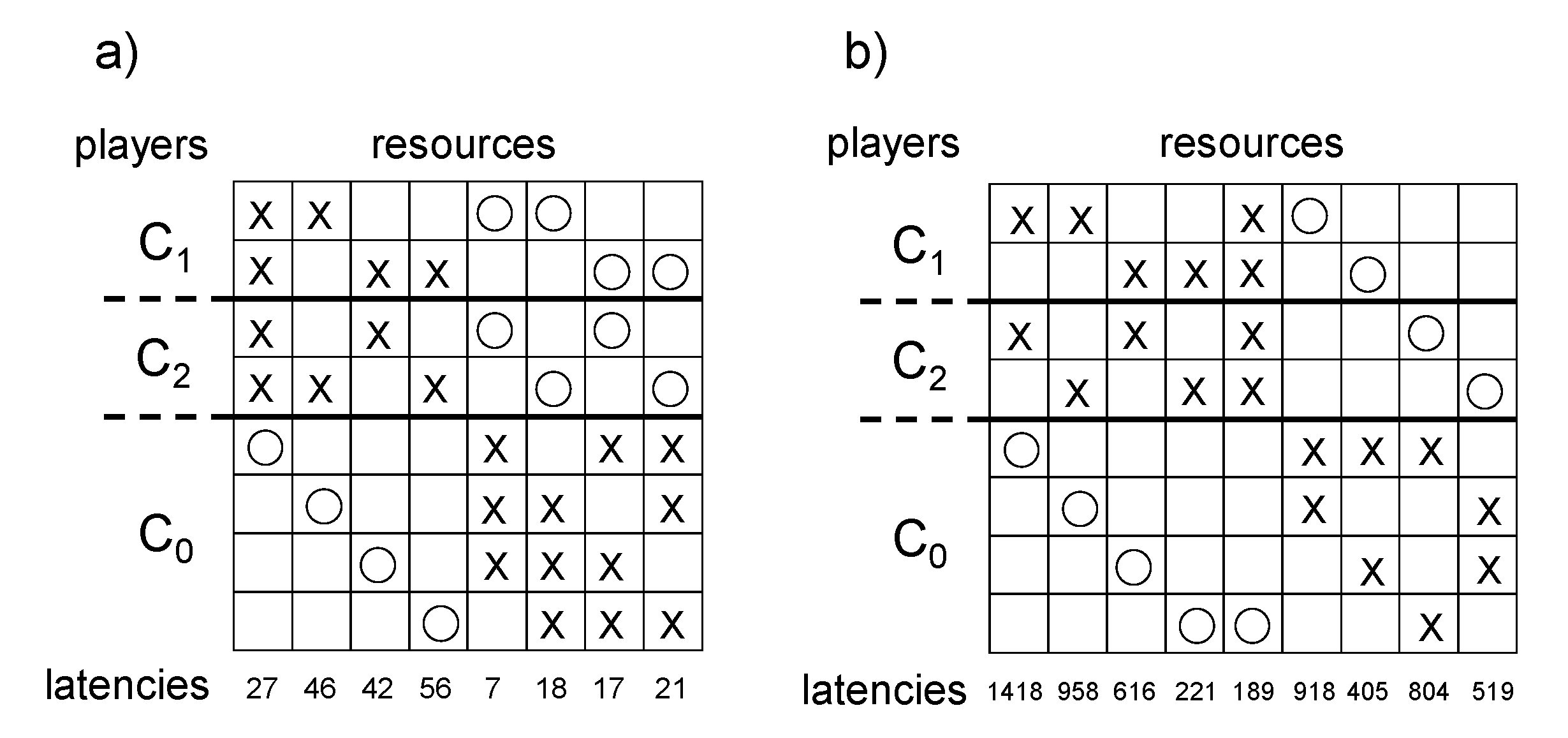
For the social cost function , consider the game depicted in Figure A1a). First, we show that is a pure Nash equilibrium for , that is, no player can lower her perceived cost by switching to her optimal strategy. Player 1 is paying ; by switching to , she pays . Player 2 is paying ; by switching to , she pays . Player 3 is paying ; by switching to , she pays . Player 4 is paying ; by switching to , she pays . Player 5 is paying ; by switching to , she pays . Player 6 is paying ; by switching to , she pays . Player 7 is paying ; by switching to , she pays . Player 8 is paying ; by switching to , she pays .
The price of anarchy of is then lower bounded by the ratio
For the social cost function , consider the game depicted in Figure A1b). First, we show that is a pure Nash equilibrium for , that is, no player can lower her perceived cost by switching to her optimal strategy. Player 1 is paying ; by switching to , she pays . Player 2 is paying ; by switching to , she pays . Player 3 is paying ; by switching to , she pays . Player 4 is paying ; by switching to , she pays . Player 5 is paying ; by switching to , she pays . Player 6 is paying ; by switching to , she pays . Player 7 is paying ; by switching to , she pays . Player 8 is paying ; by switching to , she pays .
By noting that the perceived cost of the first four players is exactly twice their presumed one, the price of anarchy of is then lower bounded by the ratio
□
Figure A1.
The games depicted in figures (a,b) represent the lower bound instances w.r.t. the social cost functions and , respectively. Each column in the matrix represents a resource of cost function whose coefficient is reported at the bottom of the column. Each row i in the matrix models the strategy set of player i as follows: circles represent resources belonging to , while crosses represent resources belonging to .

Theorem A2
(Claim of Theorem 6). For any , there exist two bidimensional linear congestion games and such that under the social cost function and under the social cost function .
Proof.
Let be a bidimensional linear congestion game such that and . Each player has two strategies and , while all players in have the same strategy .
There are three types of resources:
- resources , , each with cost function , where is an arbitrarily small positive value. Resource belongs only to ;
- resources , with , each with cost function . Resource belongs only to and to ;
- one resource with cost function . Resource belongs to for each and to .
Let (resp. ) be the strategy profile in which each player plays strategy (resp. ). The cost of each player , with , for adopting strategy when there are exactly h players in adopting the strategy played in (and thus there are players in adopting the strategy played in ) is . Similarly, the cost of each player for adopting strategy when there are exactly h players in adopting the strategy played in is . Since for any , it holds that , it follows that is the only pure Nash equilibrium for .
The price of stability of is then lower bounded by the following ratio
which, for going to infinity and , tends to .
Let be a bidimensional linear congestion game such that , and . Each player has two strategies and , while all players in have the same strategy .
There are three types of resources:
- resources , , each with cost function , where is an arbitrarily small positive value. Resource belongs only to ;
- resources , with , each with cost function . Resource belongs only to and to ;
- one resource with cost function . Resource belongs to for each and to .
Let (resp. ) be the strategy profile in which each player plays strategy (resp. ). The cost of each player for adopting strategy when there are exactly h players in adopting the strategy played in (and thus there are players in adopting the strategy played in ) is . Similarly, the cost of each player for adopting strategy when there are exactly h players in adopting the strategy played in is . Since for any , it holds that , it follows that is the only pure Nash equilibrium for .
The price of stability of is then lower bounded by the following ratio
which, for going to infinity and , tends to . □
References
- Beckmann, M.J.; McGuire, C.B.; Winsten, C.B. Studies in the Economics of Transportation; Yale University Press: London, UK, 1956. [Google Scholar]
- Rosenthal, R.W. A Class of Games Possessing Pure-Strategy Nash Equilibria. Int. J. Game Theory 1973, 2, 65–67. [Google Scholar] [CrossRef]
- Wardrop, J.G. Road Paper. Some Theoretical Aspects of Road Traffic Research. Proc. Inst. Civ. Eng. 1952, 1, 325–362. [Google Scholar] [CrossRef]
- Wardrop, J.G.; Whitehead, J.I. Correspondence. Some Theoretical Aspects of Road Traffic Research. Proc. Inst. Civ. Eng. 1952, 1, 767–768. [Google Scholar] [CrossRef]
- Nash, J.F. Equilibrium points in n-person games. Proc. Natl. Acad. Sci. USA 1950, 36, 48–49. [Google Scholar] [CrossRef] [PubMed] [Green Version]
- Koutsoupias, E.; Papadimitriou, C. Worst-case equilibria. In Proceedings of the 16th International Symposium on Theoretical Aspects of Computer Science (STACS), LNCS 1653, Trier, Germany, 4–6 March 1999; pp. 404–413. [Google Scholar]
- Anshelevich, E.; Dasgupta, A.; Kleinberg, J.; Tardos, E.; Wexler, T.; Roughgarden, T. The Price of Stability for Network Design with Fair Cost Allocation. SIAM J. Comput. 2008, 38, 1602–1623. [Google Scholar] [CrossRef]
- Aland, S.; Dumrauf, D.; Gairing, M.; Monien, B.; Schoppmann, F. Exact Price of Anarchy for Polynomial Congestion Games. SIAM J. Comput. 2011, 40, 1211–1233. [Google Scholar] [CrossRef] [Green Version]
- Awerbuch, B.; Azar, Y.; Epstein, A. The Price of Routing Unsplittable Flow. SIAM J. Comput. 2013, 42, 160–177. [Google Scholar] [CrossRef] [Green Version]
- Bhawalkar, K.; Gairing, M.; Roughgarden, T. Weighted Congestion Games: Price of Anarchy, Universal Worst-Case Examples, and Tightness. ACM Trans. Econ. Comput. 2014, 2, 14:1–14:23. [Google Scholar] [CrossRef]
- Bilò, V. A Unifying Tool for Bounding the Quality of Non-Cooperative Solutions in Weighted Congestion Games. Theory Comput. Syst. 2018, 62, 1288–1317. [Google Scholar] [CrossRef] [Green Version]
- Caragiannis, I.; Flammini, M.; Kaklamanis, C.; Kanellopoulos, P.; Moscardelli, L. Tight Bounds for Selfish and Greedy Load Balancing. Algorithmica 2011, 61, 606–637. [Google Scholar] [CrossRef]
- Christodoulou, G.; Gairing, M. Price of Stability in Polynomial Congestion Games. ACM Trans. Econ. Comput. 2016, 4, 10:1–10:17. [Google Scholar] [CrossRef]
- Christodoulou, G.; Gairing, M.; Giannakopoulos, Y.; Spirakis, P.G. The Price of Stability of Weighted Congestion Games. SIAM J. Comput. 2019, 48, 1544–1582. [Google Scholar] [CrossRef] [Green Version]
- Christodoulou, G.; Koutsoupias, E. The Price of Anarchy of Finite Congestion Games. In Proceedings of the 37th Annual ACM Symposium on Theory of Computing (STOC), Baltimore, MD, USA, 22–24 May 2005; pp. 67–73. [Google Scholar]
- Christodoulou, G.; Koutsoupias, E. On the Price of Anarchy and Stability of Correlated Equilibria of Linear Congestion Games. In Proceedings of the 13th Annual European Symposium on Algorithms (ESA), LNCS 3669, Palma de Mallorca, Spain, 3–6 October 2005; pp. 59–70. [Google Scholar]
- Christodoulou, G.; Koutsoupias, E.; Spirakis, P.G. On the Performance of Approximate Equilibria in Congestion Games. Algorithmica 2011, 61, 116–140. [Google Scholar] [CrossRef] [Green Version]
- Bilò, V.; Vinci, C. On the Impact of Singleton Strategies in Congestion Games. In Proceedings of the 25th Annual European Symposium on Algorithms (ESA), LIPIcs, Vienna, Austria, 4–6 September 2017; pp. 17:1–17:14. [Google Scholar]
- Roughgarden, T. Intrinsic Robustness of the Price of Anarchy. J. ACM 2015, 62, 32:1–32:42. [Google Scholar] [CrossRef]
- Fotakis, D.; Kontogiannis, S.; Spirakis, P. Selfish Unsplittable Flows. Theor. Comput. Sci. 2005, 348, 226–239. [Google Scholar] [CrossRef] [Green Version]
- Harks, T.; Klimm, M. On the Existence of Pure Nash Equilibria in Weighted Congestion Games. Math. Oper. Res. 2012, 37, 419–436. [Google Scholar] [CrossRef]
- Harks, T.; Klim, M.; Möhring, R.H. Characterizing the Existence of Potential Functions in Weighted Congestion Games. Theory Comput. Syst. 2011, 49, 46–70. [Google Scholar] [CrossRef]
- Bilò, V.; Fanelli, A.; Flammini, M.; Moscardelli, L. When Ignorance Helps: Graphical Multicast Cost Sharing Games. Theor. Comput. Sci. 2010, 411, 660–671. [Google Scholar] [CrossRef] [Green Version]
- Bilò, V.; Fanelli, A.; Flammini, M.; Moscardelli, L. Graphical Congestion Games. Algorithmica 2011, 61, 274–297. [Google Scholar] [CrossRef]
- Fotakis, D.; Gkatzelis, V.; Kaporis, A.C.; Spirakis, P.G. The Impact of Social Ignorance on Weighted Congestion Games. Theory Comput. Syst. 2012, 50, 559–578. [Google Scholar] [CrossRef]
- Bilò, V.; Flammini, M.; Gallotti, V. On Bidimensional Congestion Games. In Proceedings of the 19th International Colloquium on Structural Information and Communication Complexity (SIROCCO), LNCS 7355, Reykjavik, Iceland, 30 June–2 July 2012; pp. 147–158. [Google Scholar]
- Bilò, V.; Vinci, C. Dynamic Taxes for Polynomial Congestion Games. ACM Trans. Econ. Comput. 2019, 7, 15:1–15:36. [Google Scholar] [CrossRef] [Green Version]
- Caragiannis, I.; Kaklamanis, C.; Kanellopoulos, P. Taxes for linear atomic congestion games. ACM Trans. Algorithms 2010, 7, 13:1–13:31. [Google Scholar] [CrossRef] [Green Version]
- Bilò, V.; Vinci, C. On Stackelberg Strategies in Affine Congestion Games. Theory Comput. Syst. 2019, 63, 1228–1249. [Google Scholar] [CrossRef]
- Fotakis, D. Stackelberg Strategies for Atomic Congestion Games. Theory Comput. Syst. 2010, 47, 218–249. [Google Scholar] [CrossRef]
- Bell, M.G. Hyperstar: A Multi-path Astar Algorithm for Risk Averse Vehicle Navigation. Transp. Res. Part B Methodol. 2009, 43, 97–107. [Google Scholar] [CrossRef]
- Bell, M.G.; Cassir, C. Risk-averse User Equilibrium Traffic Assignment: An Application of Game Theory. Transp. Res. Part B Methodol. 2002, 36, 671–681. [Google Scholar] [CrossRef]
- Yekkehkhany, A.; Murray, T.; Nagi, R. Road Paper. Risk-Averse Equilibrium for Games. arXiv 2020, arXiv:2002.08414. [Google Scholar]
- Yekkehkhany, A.; Nagi, R. Risk-Averse Equilibrium for Autonomous Vehicles in Stochastic Congestion Games. arXiv 2020, arXiv:2007.09771. [Google Scholar]
- Bilò, V.; Moscardelli, L.; Vinci, C. Uniform Mixed Equilibria in Network Congestion Games with Link Failures. In Proceedings of the 45th International Colloquium on Automata, Languages, and Programming (ICALP), LIPIcs 107, Prague, Czech Republic, 9–13 July 2018; pp. 146:1–146:14. [Google Scholar]
- Penn, M.; Polukarov, M.; Tennenholtz, M. Congestion Games with Failures. Discret. Appl. Math. 2011, 159, 1508–1525. [Google Scholar] [CrossRef] [Green Version]
- Penn, M.; Polukarov, M.; Tennenholtz, M. Congestion Games with Load-dependent Failures: Identical Resources. Games Econ. Behav. 2009, 67, 156–173. [Google Scholar] [CrossRef] [Green Version]
Publisher’s Note: MDPI stays neutral with regard to jurisdictional claims in published maps and institutional affiliations. |
© 2020 by the authors. Licensee MDPI, Basel, Switzerland. This article is an open access article distributed under the terms and conditions of the Creative Commons Attribution (CC BY) license (http://creativecommons.org/licenses/by/4.0/).
Share and Cite
MDPI and ACS Style
Bilò, V.; Flammini, M.; Gallotti, V.; Vinci, C. On Multidimensional Congestion Games. Algorithms 2020, 13, 261. https://0-doi-org.brum.beds.ac.uk/10.3390/a13100261
AMA Style
Bilò V, Flammini M, Gallotti V, Vinci C. On Multidimensional Congestion Games. Algorithms. 2020; 13(10):261. https://0-doi-org.brum.beds.ac.uk/10.3390/a13100261
Chicago/Turabian StyleBilò, Vittorio, Michele Flammini, Vasco Gallotti, and Cosimo Vinci. 2020. "On Multidimensional Congestion Games" Algorithms 13, no. 10: 261. https://0-doi-org.brum.beds.ac.uk/10.3390/a13100261
Note that from the first issue of 2016, this journal uses article numbers instead of page numbers. See further details here.