Feasibility of Kd-Trees in Gaussian Process Regression to Partition Test Points in High Resolution Input Space


Faculty of Applied Engineering, Department Electromechanics, University of Antwerp, Groenenborgerlaan 171, B 2020 Antwerp, Belgium
*
Author to whom correspondence should be addressed.
Algorithms 2020, 13(12), 327; https://0-doi-org.brum.beds.ac.uk/10.3390/a13120327
Submission received: 21 November 2020
/
Revised: 2 December 2020
/
Accepted: 3 December 2020
/
Published: 5 December 2020
(This article belongs to the Special Issue Algorithms for Sequential Analysis)
Abstract
:Bayesian inference using Gaussian processes on large datasets have been studied extensively over the past few years. However, little attention has been given on how to apply these on a high resolution input space. By approximating the set of test points (where we want to make predictions, not the set of training points in the dataset) by a kd-tree, a multi-resolution data structure arises that allows for considerable gains in performance and memory usage without a significant loss of accuracy. In this paper, we study the feasibility and efficiency of constructing and using such a kd-tree in Gaussian process regression. We propose a cut-off rule that is easy to interpret and to tune. We show our findings on generated toy data in a 3D point cloud and a simulated 2D vibrometry example. This survey is beneficial for researchers that are working on a high resolution input space. The kd-tree approximation outperforms the naïve Gaussian process implementation in all experiments.
1. Introduction
Over the past few decades, Gaussian processes (GPs) [1] have proved themselves in a wide variety of fields: geostatistics [2], robotics and adaptive control [3], vehicle pattern recognition and trajectory modelling [4], econometrics [5], indoor map construction and localization [6], reinforcement learning [7], non-rigid shape recovery [8] and time series forecasting [9]. By following the Bayesian paradigm, they allow for a non-parametric and nonlinear regression (and classification) on only a limited set of training points. Besides being sample efficient, their predictions are more interpretable and explainable than neural networks or other conventional machine learning techniques [10]. Moreover, GPs provide predictions accompanied by an uncertainty interval. These properties are of utmost importance in the medical world [11], in finance [5] or in predictive maintenance [12]. Finally, they have a built in mechanism against overfitting [13].
The main bottleneck of GPs are the operations and storage requirements, where n is the number of training points in the dataset. This renders a naïvely implemented GP intractable for big data or growing datasets in which new data points are added sequentially. Over the last few years, the community has spent a lot of effort on tackling this hurdle. A recent and elaborate review can be found in [14]. All of the methods described approximate either the dataset or the inference itself. Once a GP has been trained, a prediction for a single test point (a point not included in the training points of the dataset) costs operations for the mean and operations for the variance [15]. This yields a second hurdle for applications where there are a lot of test points, for instance on high resolution meshes or point clouds. This is an issue for inference on measurements for example in laser Doppler vibrometry [16], micro pulse LiDAR [17], object detection [18] and spatial augmented reality tracking [19]. The computational burden grows linearly in sequential analysis where data points are added one by one. Speeding up inference time for these applications makes them more economically viable in industrial production settings like automatic quality control [20]. Whether or not naïve GPR is feasible depends on the application itself. Even small datasets with a relatively low number of test points could yield calculation times that are too long—for instance, in virtual reality where a certain frame rate needs to be achieved to prevent cyber sickness. Furthermore, a large number of calculations that add very little extra information wastes battery power. This might be an issue for internet of things devices, stand-alone head mounted displays, or drones.
One alternative to circumvent this second hurdle is to subsample the set of test points to a lower resolution. However, this results in loss of accuracy. Another approach could be to resort to implement local approximations around each of the training points. The key problem with this is that, for a high resolution set of test points, the range of each local approximation would be limited, depending on computational budget. This leads to losing the ability to learn global structures or trends. A kd-tree [21] combines the best of both worlds. It allows for a multi-resolution description of the set of test points. The nodes in the tree close to the training points are split recursively, resulting in a higher resolution in areas where the predicted posterior uncertainty is lowest. Vice versa, areas with high uncertainty fall back on lower resolution. From a Bayesian perspective, this makes total sense.
1.1. Related Work
In the literature, GPs have been constructed with multi-resolution structures in different ways. In [22], a set of smooth GPs is defined, each over a nested set of training points. A Voronoi tessellation was implemented in [23]. A kd-tree to approximate the training points in conjunction with conjugate gradient for fast inference is studied in [24]. This idea has been extended in [25] by using product trees. In [26], large scale terrain data are modeled with a kd-tree and neural network kernel to account for the non-stationary data. Distributed Gaussian processes [27] provide a divide and conquer approach by recursively distributing computations to independent computational units and then recombining them. In practice, in real time field applications, these distributed units are often not available. As for the methods in [14], all of these focus on the training points in the dataset, not on the set of test points where predictions are being made.
There exists a myriad of tree data structures such as kd-trees, octrees [28], ball trees [29] and cover trees [30]. Each have their own advantages and disadvantages. Since this work focusses on points representable by three dimensions (situated on a triangular meshes or in a point cloud), an octree or kd-tree is most applicable. In addition, locally, points on a polygon mesh that define the shape of a polyhedral object are generally not very well spread out in all three dimensions, leaving a kd-tree as the more reasonable choice.
1.2. Contribution
The main contribution of this work is validating the feasibility and efficiency of implementing a kd-tree to a set of test points that live in high resolution input space. We achieve this by:
- showing that the kd-tree approximation can lead to considerable time savings without sacrificing much accuracy.
- proposing a cut-off rule by combining criteria that are easy to interpret and that can be tailored for different computational budgets.
- applying our method in a sequential analysis setting on two types of generated toy data: a 3D point cloud with hotspots and a simulated 2D laser Doppler vibrometry example.
To the best of our knowledge, no work has been done earlier on kd-trees approximating the set of test points in Gaussian process regression.
1.3. Outline of the Paper
This paper is structured as follows. In Section 2, we present a brief overview of Gaussian processes. In Section 3, we propose our method for kd-tree construction and cut-off rule. We validate our findings on experiments in Section 4. We discuss the results and future work in Section 5 and make conclusions in Section 6.
2. Gaussian Processes
2.1. Gaussian Process Regression
By definition, a Gaussian process (GP) is a continuous collection of random variables, any finite subset of which is normally distributed as a multivariate distribution. A more comprehensive treatment can be found in [1]. Here, we give a brief introduction with focus on practical implications.
Let be a dataset of n observations, where is an matrix of n input vectors of dimension d and is a vector of continuous-valued scalar outputs. These data points are also called training points. Regression aims to find a mapping ,
with being identically distributed observation noise. In stochastic numerics, this mapping is often implemented by a Gaussian process, which is fully defined by its mean and covariance function . It is generally denoted as . Typically, the covariance function, also referred to as a kernel or kernel function, is parametrized by a vector of hyperparameters . By definition, a GP yields a distribution over a collection of functions that have a joint normal distribution [1],
where X and are the input vectors of the n observed training points and the unobserved test points, respectively. The vectors of mean values for X and are given by and . The covariance matrices , , and are constructed by evaluating k at their respective pairs of points. In practice, we don’t have access to the latent function values directly, but are dependent on the noisy observations .
Putting it all together, the conditional (predictive posterior) distribution of the GP can be written as:
Without loss of generality, the mean function m is often set to zero. This does not imply a zero mean posterior , which in fact does not depend on the mean of the training points at all. However, recent work by [31] shows that the rate of convergence for Bayesian optimization (BO) can depend sensitively on the choice for a non-zero mean function.
An extensive overview of kernels and how to implement and combine them can be found in [32]. Hyperparameters are usually learned by using a gradient based optimization algorithm to maximize the log marginal likelihood,
which is a combination of a data fit term and complexity penalty and thus automatically incorporates Occam’s Razor [33]. This guards the GP against overfitting. A comparison of common optimizers can be found in [34]. In our experiments, we use BFGS, a quasi-Newton method described in [35].
For efficiency and numerical stability, the linear system is often calculated by first calculating the Cholesky decomposition factor L of and then solving
2.2. Covariance Functions
There exists a large variety of kernel functions, which have been extensively studied and reviewed in [36]. The de facto default kernel used in Gaussian processes is the squared exponential kernel, also called the radial basis function kernel, the Gaussian kernel, or exponentiated quadratic kernel. It is applicable in a wide variety of situations because it is infinitely differentiable and thus yields smooth functions. Besides that, it only takes two hyperparameters to tune. It has the form:
in which is a height-scale factor and l the length-scale that determines the radius of influence of the training points. For the squared exponential kernel, the hyperparameters are . For the function to be a valid kernel, it must be positive semi-definite (PSD), which means that, for any vector , the kernel matrix K is positive semi-definite. This implies that for all . In this work, we only use the squared exponential kernel.
2.3. Computational and Memory Requirements
Gaussian processes regression (GPR) requires operations and storage [15], making it an intractable method for datasets that contain over a few thousand training points. Over the past few decades, a considerable amount of work has been done by the community to overcome this problem. A thorough review can be found in [14]. Big datasets are not an issue in our research, as we aim to gain a maximum amount of information about a large number of test points on a mesh or point cloud by using as few training points as possible. We typically restrict ourselves to . This leads to a matrix of moderate size . Contrarily, in this work, we study the challenge of having test points, resulting in a large matrix of size and a matrix of size (and its transpose). The predictive mean and variance of a trained GP cost and operations per test point [15], resulting in and . Practical applications generally do not require the full predictive covariance matrix, but rather the predictive variance along its diagonal. This reduces the calculation of the values of to only the diagonal values. The main contribution of this work is the feasibility of implementing a kd-tree to approximate the set of test points and thus reducing all together. In sequential analysis, this computational gain adds up quickly. For every new incoming data point, n increases by one and both and have to be recalculated again.
3. Kd-Trees
The main goal of using kd-trees in our research is to implement a structure that yields a set of test points with higher resolution around the training points and lower resolution in areas far away from the data. From a Bayesian perspective, this makes sense. Predictions in areas far away from the data tend to fall back on the prior, and thus have greater associated uncertainty. Our main philosophy is that we can trade off many time-consuming predictions with large uncertainty for fewer predictions and thus speedier inference—even if those predictions are less accurate due to the approximation of the structure. In our experiments, we iteratively add training points, retrain the GP each time (calculate all covariance matrices) and infer the posterior distribution on the relevant nodes in the tree instead of all the test points on the mesh.
3.1. Construction
A kd-tree [37] for a set X is a binary tree with the nodes labelled by non-empty subsets of X, following the conditions:
- label(root) = X, the whole set
- label(leaf) = , one point
- label(internal node) = label(left child) ⊔ label(right child), the disjoint union of the sets below
In our work, we apply the kd-tree to the set of all test points (not the set of all training points). Typically, these are part of a triangular mesh and thus represent positions in three-dimensional Euclidean space. Therefore, a node can be described by a bounding rectangular box or cuboid. Several possible splitting criteria have been proposed to split the nodes recursively [21]. As described in detail in [38], a commonly used method is splitting a node along the median of its widest dimension. For a balanced kd-tree, in each node. Balancing a kd-tree optimizes search times for random points [39]. Nearest neighbour search in a kd-tree with randomly distributed points takes an empirically observed average running time of [40].
For trees with large nodes, as in our case, calculating the median becomes time-consuming. According to [41], a faster approach to construct the kd-tree is splitting a node in half along its widest dimension. However, this approach does not guarantee a balanced tree. Nonetheless, the imbalances observed when working with points that are spread evenly on a high resolution triangular mesh are negligible. This approach is also explained in [42,43]. Alternatively, Ref. [39] also states that simply alternating the dimension to split along would be even faster, since this eliminates the need to check for the widest dimension or calculating the median. Locally, triangular meshes become almost flat 2D surfaces. Using all three dimensions in an alternating way introduces very underpopulated nodes. These imbalances have a negative effect on overall performance. However, for point clouds that do not represent a 2D surface embedded in 3D, this is a viable alternative.
In our implementation, the kd-tree is fixed and fully constructed beforehand. Alternatively, the kd-tree could be adaptive to incoming data points, expanding nodes only when needed, i.e., when they are close to data points according to the criteria mentioned. We leave this for future work.
3.2. Cut-Off Rule
When iterating through the tree, i.e., when determining which nodes to use in GPR, the decision to descend to a child node is determined by a cut-off rule. The design of this rule is crucial for both performance and accuracy. In our implementation, we take different criteria into consideration and define several easy to configure parameters. Working with multiple criteria and parameters has the advantage that the decision-making process is more interpretable. Furthermore, in our code implementation, we postpone more time-consuming calculations to when they are necessary. The most important criterion is how close a training point is to the node under evaluation. The cut-off rule determines whether a node is retained or the algorithm should recursively descend to the node’s children. When iterating through the nodes of the tree, we evaluate every training point from the dataset one by one. When for a training point a criterion is met to descend further in the tree to the node’s children, we no longer check the remaining training points. We flag the decision for a node to descend further into its children for future iterations.
For the first cut-off criterion, we calculate the covariance between the node’s minimum and maximum point along its widest dimension and ,
in which k is the GP kernel function and h is its height-scale for normalization. This results in a value between 0 and 1 and serves as a measurement for how wide the cuboid encapsulating the node is. If this value is above a threshold , then there is significant covariance between the two extrema. This case we are considering a node with points that are close to each other, so it is retained and the recursion is cut off. Otherwise, the algorithm continues to descend into the child nodes. This yields the first cut-off criterion:
It puts an upper limit on the size we allow for the cuboids encapsulating the nodes. Cuboids that are too large make the kd-tree approximation too crude.
For the second cut-off criterion, we calculate the covariance between the training point and the node’s representative point . In our case, this is the nearest neighbour to the arithmetic mean of the points in the node. This representative point is pre-calculated when the tree is constructed and stored in the node itself. By using the nearest neighbour, we ensure that is a point on the mesh:
Again, we have an easy to interpret value between 0 and 1 that can be seen as a measurement for the distance between the node and the training point. If this value is below a certain threshold , then the node is far from the training point, so it is retained and the recursion is cut off. Otherwise, we continue. This yields the second cut-off criterion:
This puts a lower limit on the distance we allow for the nodes. Nodes that are too close are not retained, unless they are a leaf. In other words, close to the training points, we abandon the kd-tree and work with the actual test points.
By including the kernel in the above criteria, it becomes part of the cut-off rule itself. The thresholds adapt to the kernel length-scale and height-scale. A downside to this approach is that these thresholds have to be recalculated every time the hyperparameters of the kernel function are updated.
The first two criteria implement strict boundaries: nodes with cuboids that are too large or nodes that are too close to the data points are not retained. This means their child nodes are always visited. A third cut-off criterion further investigates the nodes that are retained. It builds on the second criterion, by feeding through a sigmoid function to yield:
in which s is a steepness factor and m is a shift of the midpoint. This allows us to tune the outcome of the first two all-or-nothing criteria. Finally, it is evaluated against the relative depth of the node in the third cut-off criterion:
This way, shallow nodes are evaluated against a lower threshold, making them less likely to be retained.
Lastly, whenever we encounter a node without children, a leaf, we can no longer recursively iterate further. This node is always retained. In the limit, when all the retained nodes are leaves, the kd-tree approximation results in the full set of test points. Our overall algorithm is summarized in Algorithm 1.
| Algorithm 1 Get Nodes In Kd-Tree | |
| 1: | ▹ start with an empty list of tree nodes |
| 2: | ▹ start recursion |
| 3: return | |
| 4: procedure GetNodesInBranch(node) | |
| 5: | ▹ empty list of branch nodes |
| 6: if node.isLeaf then | |
| 7: | |
| 8: return | |
| 9: else | |
| 10: if node.mustVisitChildren then | ▹ if flag set in previous iteration |
| 11: | |
| 12: | |
| 13: return | |
| 14: else | |
| 15: for all do | ▹ evaluate every training point |
| 16: if then | ▹ node too wide |
| 17: node.mustVisitChildren ← True | |
| 18: | ▹ no need to evaluate other training points |
| 19: else if then | ▹ node too close |
| 20: node.mustVisitChildren ← True | |
| 21: | ▹ no need to evaluate other training points |
| 22: else if then | |
| 23: node.mustVisitChildren ← True | |
| 24: | ▹ no need to evaluate other training points |
| 25: end if | |
| 26: end for | |
| 27: if node.mustVisitChildren then | ▹ recursion continues |
| 28: | |
| 29: | |
| 30: else | ▹ recursion is cut off |
| 31: | |
| 32: end if | |
| 33: return | |
| 34: end if | |
| 35: end if | |
| 36: end procedure |
In our implementation, we constructed a class named KDNode of which the most important elements are
- references to the left and right child nodes which are also objects of the class KDNode
- a boolean indicating the node is a leaf or not
- for the leaves the position of the point
- the position of the nearest neighbour in the node to the average position, i.e., the representative point
- a boolean whether the child nodes should be visited by the algorithm
- the pre-calculated covariance between the two most distant points in the node
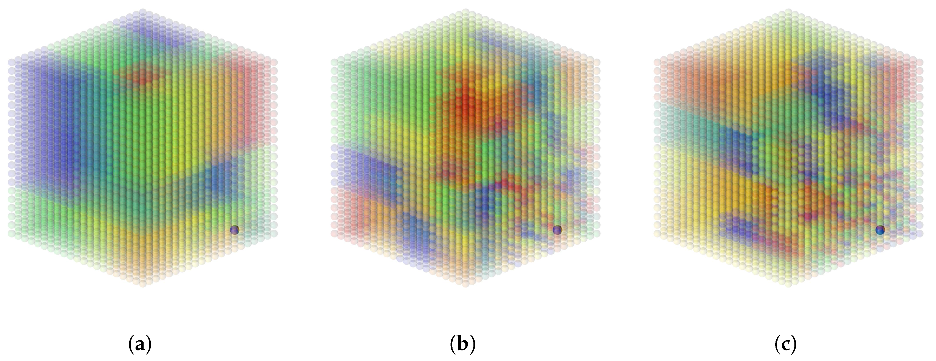
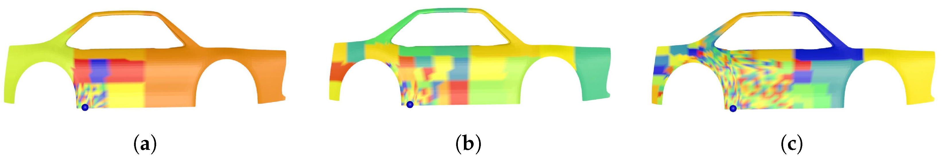
We implemented a module that renders a random colour for every node returned by our algorithm. This allows for visual tuning of the kd-tree parameters. Examples of a constructed kd-tree are given in Figure 1 and Figure 2. By tuning s and m, we can tailor the kd-tree to every computational budget. Furthermore, we can have a boundary with a steepness that corresponds to the behaviour of the covariance function used.
4. Results
We performed experiments on two types of generated toy data: a 3D point cloud with hotspots and a simulated 2D laser Doppler vibrometry example. All experiments were run in the editor of the Unity game engine [44] version 2019.2.17f1. All code was written in C#, which automatically gets recompiled to C++. For mathematical functionality, we imported the open source library Math.NET Numerics [45]. We used a laptop with an i7 9th Gen Intel processor, a GTX 2080 graphics card and 32 GB RAM. This setup is not the most performant. It does, however, facilitate the visualization of the different models and allows us to assess whether or not these techniques could be used in practical virtual or augmented reality applications for which Unity is currently a widely used development tool. We investigated GPR by sequentially adding training points. Each step is called an iteration. To make the comparison between the naïve GP and the kd-tree implementation fair, we always started both runs at the same initial training point. The point with the highest posterior uncertainty was chosen as the next new training point. This is the point where the least is known about the underlying function. This is the fastest way to reduce the total uncertainty with every new data point. To assess the merit of the kd-tree, we logged two values.
First, we calculated the normalized root mean square error (NRMSE) between the ground truth and the posterior mean via
in which the root mean square error RMSE (between the ground truth values y and the predicted values ) is normalized by the average ground truth value . This is a measurement for how far the GPR prediction deviates from the ground truth.
Second, we calculated the average value for all points (both test and training). For a normal distribution, 95% of the samples lie within a band around the mean with a width of two standard deviations . This is a measurement for how much uncertainty the posterior still has for our input domain and thus how much information could be gained by continuing the regression. When this value converges, there is little use in continuing.
Hyperparameters were learned beforehand and not updated during inference. This strategy is explained in [46]. Updating between iterations while the dataset is small can lead to length-scales that are too big and predictions that are overconfident far from the data itself. Moreover, because learning the hyperparameters via BFGS depends on numerical convergences, this would result in varying iteration times, making a comparison between them futile. Instead, hyperparameters were learned on a portion of the data set. We took 100 evenly spread out training points and learned the hyperparameters on those. We then adjusted them to reasonable values’ encapsulation prior belief. A kernel noise of was used throughout.
In these experiments, we set to 0, meaning we allowed encapsulating cuboids to be of any size. The choice of s and m removed the need to impose a stricter threshold. However, this might not always be the case. This depends on the application. Choosing a larger value puts an upper limit on the size of the cuboids, resulting in a minimum resolution of the spread of the test points. For , a value of 1 was chosen, which allows for nodes to be far from the data points. Choosing a lower number means abandoning the kd-tree for nodes that are close to the data points.
4.1. Generated Data on a 3D Point Cloud
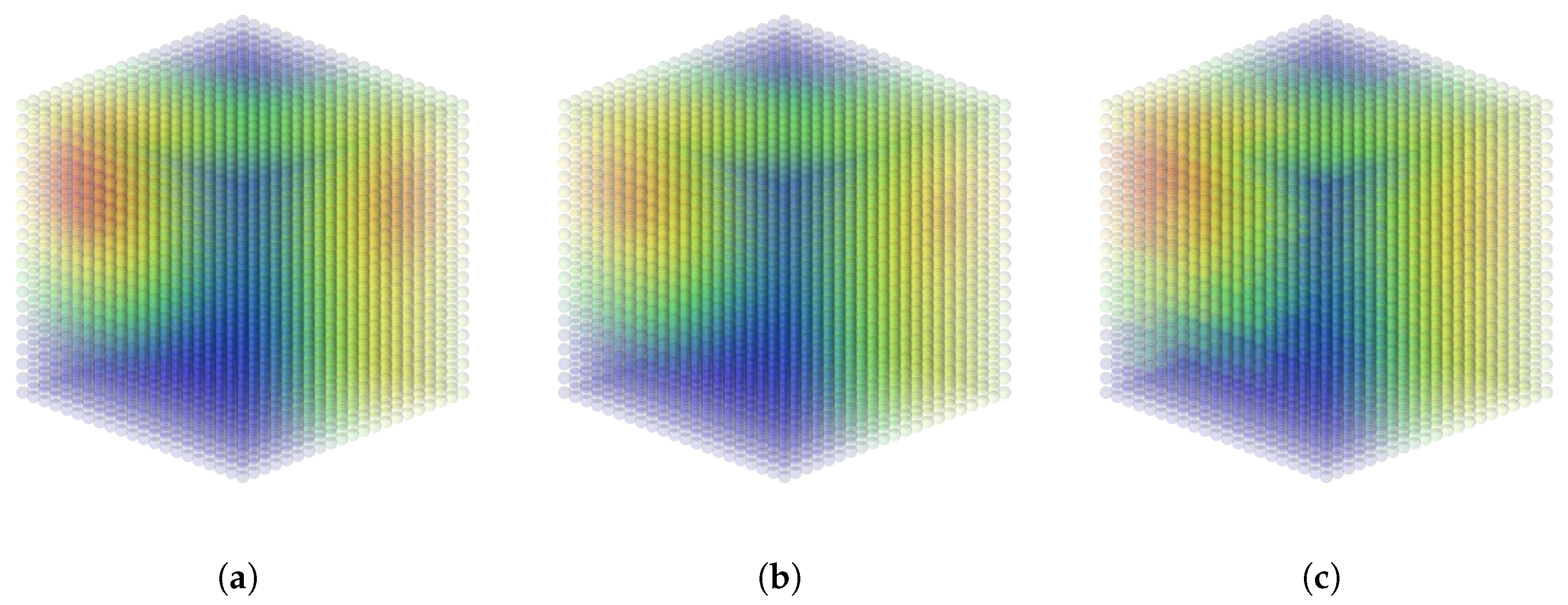
We generated toy data by simulating heat in a 3D point cloud in which 9261 points are organized in a cubic grid. From its points, we picked three and assigned each one a toy value of , and , respectively. These functioned as simulated sources of heat. We then calculated a dummy heat value in every other point using the heat kernel as described in [47]. For simplicity, we used Euclidean distances. This serves as a function in 3D with three local maxima. This model is referenced by the name Cube. A visualization is given in Figure 3.
Via GPR, we inferred the generated heat values for every point in the point cloud. We started with just one training point which was the point with the lowest local maximum of . We choose the squared exponential covariance function since it behaves similarly to the heat kernel. The height scale was set to and the length scale to . We ran 100 iterations in total. Each iteration added a new training point taken from the ground truth. The time to construct the kd-tree beforehand was ms.
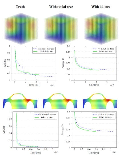
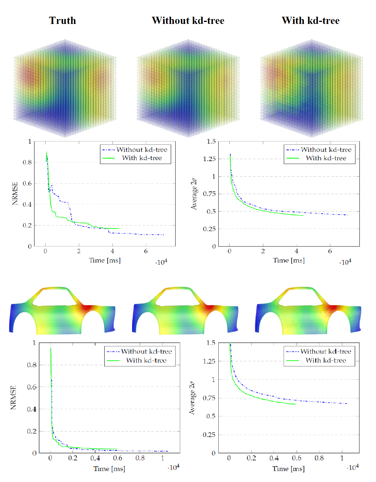
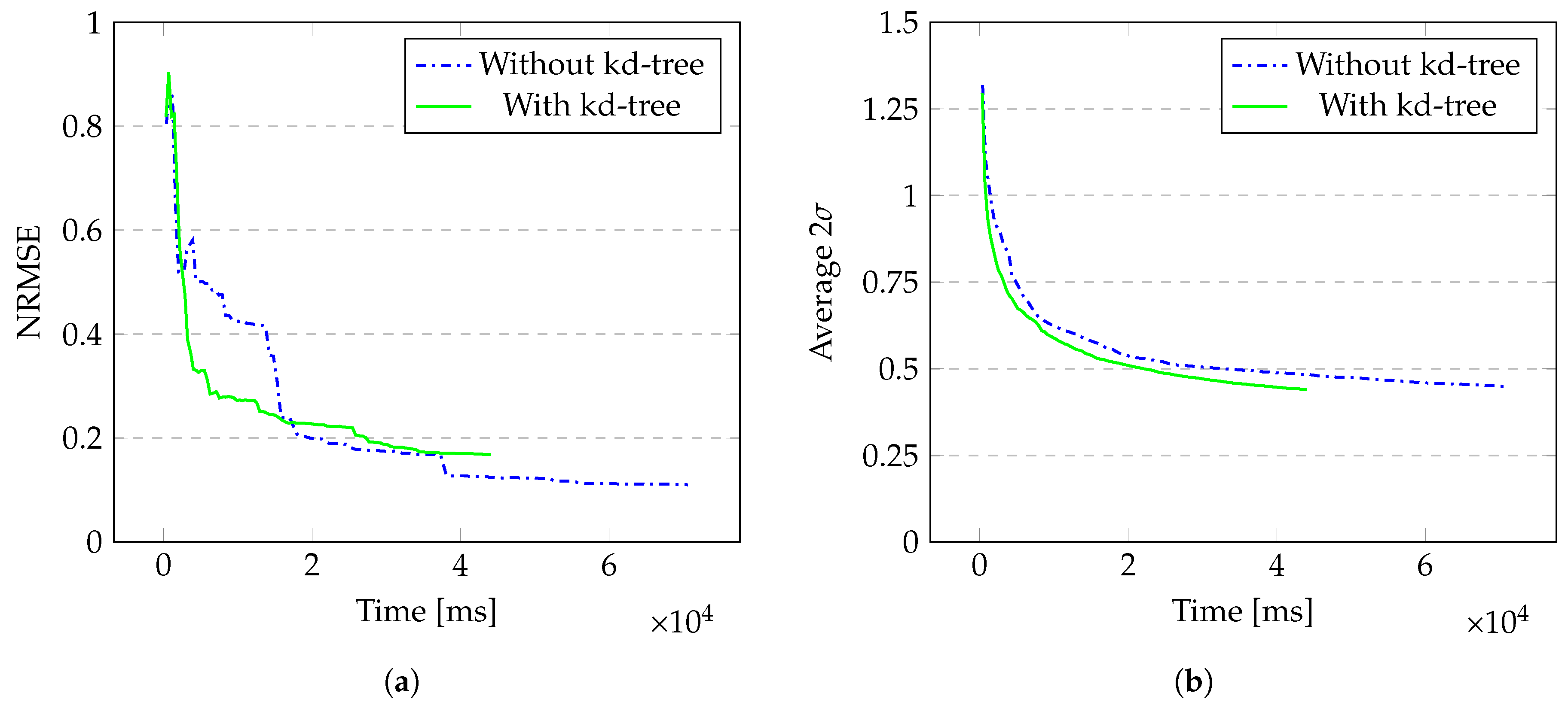
As can be seen in Figure 4 and Table 1, Table 2 and Table 3, the kd-tree approximation is slightly less accurate but almost 38 percent faster with similar values for the uncertainty level. The time compared is the time spent on GPR calculations, not the total time the application ran. This filters out the time Unity needed to render the spheres and other graphical elements in our scene that are besides the implementation of the kd-tree analysis. This gain in GPR calculation time highly depends on the number of iterations, as the covariance matrices grow faster for the naïve GPR in comparison to the kd-tree implementation.
4.2. Laser Doppler Vibrometry Simulation
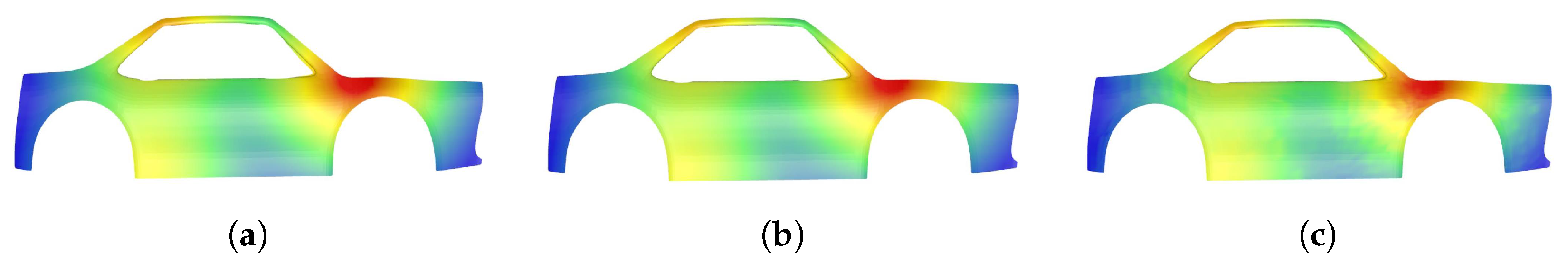
In a second experiment, we simulated a laser Doppler vibrometry setup. We used Blender to model the side frame of a car. The triangular mesh consisted of 2296 vertices. These serve as the locations of the input points. Again, we picked three of those and assigned each one a toy value of , and , respectively. As in the experiment above, we then calculated a dummy value in every other point. In a real world situation, these could be vibration amplitudes as for instance described in [16]. This model is referenced by the name Car. A visualization is given in Figure 5.
Via GPR, we inferred the generated heat values for every point in the point cloud. We started with just one training point which was the point with the lowest local maximum of . We choose the squared exponential covariance function since it behaves similarly to the heat kernel. The height scale was set to and the length scale to . We ran 100 iterations in total. Each iteration added a new training point taken from the ground truth. The time to construct the kd-tree beforehand was ms.
5. Discussion
In this work, we focussed on implementing a kd-tree in Gaussian process regression. However, this technique could also be used in classification scenario’s or when working with non-stationary data. Further work is required to establish the viability in these settings. Furthermore, it is an open question whether or not the approximations can be used with non-stationary data, as large nodes tend to hide underlying local trends like a change in the frequency spectrum of the underlying latent function. In our dataset, the number of dimensions remained restricted to three. Moreover, points on a polygon mesh are locally almost coplanar. This makes the kd-tree a reasonable choice. A comparison to other tree-like structures could confirm this.
We implemented a fixed kd-tree that is constructed beforehand. Alternatively, the kd-tree could be adaptive to sequentially incoming data points. We permanently flag the decision for a node to descend further into its children. Future iterations use this flag to bypass the calculations for the criteria. In our experiments, we gradually introduce new data points one by one. This results in an ever growing set of retained test points. Alternatively, one could implement Bayesian filtering techniques explained in [48,49] to combine the previously calculated posterior with a new one based on only one data point and a new set of test points.
In our experiments, we restricted the dataset to 100 data points. The issue of large datasets is beyond the scope of this paper. Further studies regarding the incorporation of the techniques presented in [14] would be worthwhile. This would lower both the amount of data points and test points simultaneously, resulting in even larger computational gains.
This work can be extended to points on graphs such as representations of computer networks or links between people both in real life or on social media. An application of this is monitoring the spread of contagious diseases like for example Covid-19 among a population with only limited testing.
6. Conclusions
The main goal of this work was to determine the feasibility of implementing a kd-tree in Gaussian process regression on a set of test points in scenarios where the input space has so many points that inference becomes slow. This is, for instance, the case when working with a high resolution triangular mesh or large point cloud. From a Bayesian perspective, the kd-tree implementation is justified by approximation regions with higher uncertainty more crudely than regions close to the training points. It takes extra time to construct a kd-tree, especially for higher resolution input spaces. However, our experiments confirmed that this allows for faster inference while sacrificing only little accuracy. It is always worth the time investment. The larger the number of test points to make predictions for, the larger the gain by using a kd-tree. This allows for inference on high resolution meshes which would otherwise not be possible within reasonable time constraints. We proposed a cut-off rule combined of easy to interpret and tune criteria and demonstrated this on generated data. The kd-tree always outperforms the naïve GP implementation. The need for more accuracy can be satisfied by making the kd-tree approximation less crude. We showed that this can be easily accomplished by tuning the kd-tree construction parameters. This allows for a trade-off between accuracy and speed suited for every computational budget. In summary, these results show that the kd-tree implementation can speed up the inference process significantly without sacrificing too much accuracy.
Author Contributions
Conceptualization, I.D.B. and R.P.; methodology, I.D.B. and R.P.; software, I.D.B.; validation, I.D.B.; formal analysis, I.D.B.; investigation, I.D.B.; resources, I.D.B.; data curation, I.D.B.; writing—original draft preparation, I.D.B.; writing—review and editing, I.D.B., R.P., P.J. and B.R.; visualization, I.D.B; supervision, R.P.; project administration, B.R.; funding acquisition, R.P and B.R. All authors have read and agreed to the published version of the manuscript.
Funding
This research received no external funding.
Acknowledgments
We thank the anonymous reviewers whose comments helped improve the quality of this paper.
Conflicts of Interest
The authors declare no conflict of interest.
References
- Rasmussen, C.E.; Williams, C.K.I. Gaussian Processes for Machine Learning (Adaptive Computation and Machine Learning); The MIT Press: Cambridge, MA, USA, 2005. [Google Scholar]
- Matheron, G. Principles of geostatistics. Econ. Geol. 1963, 58, 1246–1266. [Google Scholar] [CrossRef]
- Jaquier, N.; Rozo, L.; Calinon, S.; Bürger, M. Bayesian optimization meets Riemannian manifolds in robot learning. In Proceedings of the Conference on Robot Learning, Cambridge MA, USA, 16–18 November 2020; pp. 233–246. [Google Scholar]
- Tiger, M.; Heintz, F. Gaussian Process Based Motion Pattern Recognition with Sequential Local Models. In Proceedings of the 2018 IEEE Intelligent Vehicles Symposium (IV), Changshu, China, 26–30 June 2018; pp. 1143–1149. [Google Scholar]
- Mojaddady, M.; Nabi, M.; Khadivi, S. Stock market prediction using twin Gaussian process regression. Int. J. Adv. Comput. Res. (JACR) Preprint 2011. Available online: http://disi.unitn.it/~nabi/files/stock.pdf (accessed on 4 December 2020).
- Wang, X.; Wang, X.; Mao, S.; Zhang, J.; Periaswamy, S.C.; Patton, J. Indoor Radio Map Construction and Localization with Deep Gaussian Processes. IEEE Internet Things J. 2020, 7, 11238–11249. [Google Scholar] [CrossRef]
- Brochu, E.; Cora, V.M.; De Freitas, N. A tutorial on Bayesian optimization of expensive cost functions, with application to active user modeling and hierarchical reinforcement learning. arXiv 2010, arXiv:1012.2599. [Google Scholar]
- Zhu, J.; Hoi, S.C.; Lyu, M.R. Nonrigid shape recovery by gaussian process regression. In Proceedings of the 2009 IEEE Conference on Computer Vision and Pattern Recognition, Miami, FL, USA, 20–25 June 2009; pp. 1319–1326. [Google Scholar]
- Hachino, T.; Kadirkamanathan, V. Multiple Gaussian process models for direct time series forecasting. IEEJ Trans. Electr. Electron. Eng. 2011, 6, 245–252. [Google Scholar] [CrossRef]
- Plate, T.A. Accuracy versus interpretability in flexible modeling: Implementing a trade-off using gaussian process models. Behaviormetrika 1999, 26, 29–50. [Google Scholar] [CrossRef] [Green Version]
- Lasko, T.A. Efficient inference of Gaussian-process-modulated renewal processes with application to medical event data. In Uncertainty in Artificial Intelligence: Proceedings of the Conference on Uncertainty in Artificial Intelligence; NIH Public Access: Bethesda, MD, USA, 2014; Volume 2014, p. 469. [Google Scholar]
- Aye, S.; Heyns, P. An integrated Gaussian process regression for prediction of remaining useful life of slow speed bearings based on acoustic emission. Mech. Syst. Signal Process. 2017, 84, 485–498. [Google Scholar] [CrossRef]
- Mohammed, R.O.; Cawley, G.C. Over-fitting in model selection with gaussian process regression. In Proceedings of the International Conference on Machine Learning and Data Mining in Pattern Recognition, New York, NY, USA, 15–20 July 2017; Springer: Berlin/Heidelberg, Germany, 2017; pp. 192–205. [Google Scholar]
- Liu, H.; Ong, Y.S.; Shen, X.; Cai, J. When Gaussian process meets big data: A review of scalable GPs. IEEE Trans. Neural Netw. Learn. Syst. 2020, 31, 4405–4423. [Google Scholar] [CrossRef] [Green Version]
- Wilson, A.G.; Dann, C.; Nickisch, H. Thoughts on massively scalable Gaussian processes. arXiv 2015, arXiv:1511.01870. [Google Scholar]
- Rothberg, S.; Allen, M.; Castellini, P.; Di Maio, D.; Dirckx, J.; Ewins, D.; Halkon, B.J.; Muyshondt, P.; Paone, N.; Ryan, T.; et al. An international review of laser Doppler vibrometry: Making light work of vibration measurement. Opt. Lasers Eng. 2017, 99, 11–22. [Google Scholar] [CrossRef] [Green Version]
- Spinhirne, J.D. Micro pulse lidar. IEEE Trans. Geosci. Remote. Sens. 1993, 31, 48–55. [Google Scholar] [CrossRef]
- Shi, S.; Wang, Z.; Shi, J.; Wang, X.; Li, H. From points to parts: 3d object detection from point cloud with part-aware and part-aggregation network. IEEE Trans. Pattern Anal. Mach. Intell. 2020. [Google Scholar] [CrossRef] [PubMed] [Green Version]
- Chadalavada, R.T.; Andreasson, H.; Schindler, M.; Palm, R.; Lilienthal, A.J. Bi-directional navigation intent communication using spatial augmented reality and eye-tracking glasses for improved safety in human–robot interaction. Robot. Comput. Integr. Manuf. 2020, 61, 101830. [Google Scholar] [CrossRef]
- Paone, N.; Scalise, L.; Stavrakakis, G.; Pouliezos, A. Fault detection for quality control of household appliances by non-invasive laser Doppler technique and likelihood classifier. Measurement 1999, 25, 237–247. [Google Scholar] [CrossRef]
- Ramasubramanian, V.; Paliwal, K.K. A generalized optimization of the K-d tree for fast nearest-neighbour search. In Proceedings of the Fourth IEEE Region 10 International Conference TENCON, Bombay, India, 22–24 November 1989; pp. 565–568. [Google Scholar]
- Fox, E.; Dunson, D.B. Multiresolution gaussian processes. Adv. Neural Inf. Process. Syst. 2012, 25, 737–745. [Google Scholar]
- Kim, H.M.; Mallick, B.K.; Holmes, C. Analyzing nonstationary spatial data using piecewise Gaussian processes. J. Am. Stat. Assoc. 2005, 100, 653–668. [Google Scholar] [CrossRef]
- Shen, Y.; Seeger, M.; Ng, A.Y. Fast gaussian process regression using kd-trees. Adv. Neural Inf. Process. Syst. 2006, 18, 1225–1232. [Google Scholar]
- Moore, D.A.; Russell, S.J. Fast Gaussian Process Posteriors with Product Trees. In Proceedings of the UAI, Quebec City, QC, Canada, 23–27 July 2014; pp. 613–622. [Google Scholar]
- Vasudevan, S.; Ramos, F.; Nettleton, E.; Durrant-Whyte, H. Gaussian process modeling of large-scale terrain. J. Field Robot. 2009, 26, 812–840. [Google Scholar] [CrossRef]
- Deisenroth, M.; Ng, J.W. Distributed gaussian processes. In Proceedings of the International Conference on Machine Learning, Lille, France, 6–11 July 2015; pp. 1481–1490. [Google Scholar]
- Yamaguchi, K.; Kunii, T.; Fujimura, K.; Toriya, H. Octree-related data structures and algorithms. IEEE Comput. Graph. Appl. 1984, 53–59. [Google Scholar] [CrossRef]
- Omohundro, S.M. Five Balltree Construction Algorithms; International Computer Science Institute: Berkeley, CA, USA, 1989. [Google Scholar]
- Beygelzimer, A.; Kakade, S.; Langford, J. Cover trees for nearest neighbour. In Proceedings of the 23rd International Conference on Machine Learning, Pittsburgh, PA, USA, 25–29 June 2006; pp. 97–104. [Google Scholar]
- De Ath, G.; Fieldsend, J.E.; Everson, R.M. What Do You Mean? The Role of the Mean Function in Bayesian Optimisation. In Proceedings of the 2020 Genetic and Evolutionary Computation Conference Companion (GECCO ’20), Cancún, Mexico, 8–12 July 2020; Association for Computing Machinery: New York, NY, USA, 2020; pp. 1623–1631. [Google Scholar] [CrossRef]
- Duvenaud, D. Automatic Model Construction with Gaussian Processes. Ph.D. Thesis, Computational and Biological Learning Laboratory, University of Cambridge, Cambridge, UK, 2014. [Google Scholar]
- Rasmussen, C.; Ghahramani, Z. Occam’s Razor. In Advances in Neural Information Processing Systems 13; Max-Planck-Gesellschaft, MIT Press: Cambridge, MA, USA, 2001; pp. 294–300. [Google Scholar]
- Blum, M.; Riedmiller, M.A. Optimization of Gaussian process hyperparameters using Rprop. In Proceedings of the ESANN, Bruges, Belgium, 24–26 April 2013; pp. 339–344. [Google Scholar]
- Liu, D.C.; Nocedal, J. On the limited memory BFGS method for large scale optimization. Math. Program. 1989, 45, 503–528. [Google Scholar] [CrossRef] [Green Version]
- Genton, M.G. Classes of Kernels for Machine Learning: A Statistics Perspective. J. Mach. Learn. Res. 2002, 2, 299–312. [Google Scholar]
- Preparata, F.P.; Shamos, M.I. Computational Geometry: An Introduction; Springer Science & Business Media: Berlin/Heidelberg, Germany, 2012. [Google Scholar]
- Zhou, K.; Hou, Q.; Wang, R.; Guo, B. Real-Time KD-Tree Construction on Graphics Hardware. ACM Trans. Graph. 2008, 27. [Google Scholar] [CrossRef]
- Friedman, J.H.; Bentley, J.L.; Finkel, R.A. An Algorithm for Finding Best Matches in Logarithmic Expected Time. ACM Trans. Math. Softw. 1977, 3, 209–226. [Google Scholar] [CrossRef]
- Bentley, J.L. Multidimensional Binary Search Trees Used for Associative Searching. Commun. ACM 1975, 18, 509–517. [Google Scholar] [CrossRef]
- Sproull, R. Refinements to nearest-neighbour searching ink-dimensional trees. Algorithmica 1991, 6, 579–589. [Google Scholar] [CrossRef]
- Sample, N.; Haines, M.; Arnold, M.; Purcell, T. Optimizing Search Strategies in k-d Trees. Available online: http://infolab.stanford.edu/~nsample/pubs/samplehaines.pdf (accessed on 4 December 2020).
- Deng, K.; Moore, A. Multiresolution Instance-Based Learning. In Proceedings of the IJCAI, Montreal, QC, Canada, 20–25 August 1995. [Google Scholar]
- Haas, J.K. A History of the Unity Game Engine. 2014. Available online: https://web.wpi.edu/Pubs/E-project/Available/E-project-030614-143124/unrestricted/Haas_IQP_Final.pdf (accessed on 4 December 2020).
- Ruegg, C.; Cuda, M.; Van Gael, J. Math .NET Numerics. 2016. Available online: http://numerics.mathdotnet.com (accessed on 4 December 2020).
- Ram, R.; Müller, S.; Pfreundt, F.; Gauger, N.R.; Keuper, J. Scalable Hyperparameter Optimization with Lazy Gaussian Processes. In Proceedings of the 2019 IEEE/ACM Workshop on Machine Learning in High Performance Computing Environments (MLHPC), Denver, CO, USA, 18 November 2019; pp. 56–65. [Google Scholar]
- Crane, K.; Weischedel, C.; Wardetzky, M. Geodesics in Heat: A New Approach to Computing Distance Based on Heat Flow. ACM Trans. Graph. 2013, 32. [Google Scholar] [CrossRef]
- Sarkka, S.; Solin, A.; Hartikainen, J. Spatiotemporal Learning via Infinite-Dimensional Bayesian Filtering and Smoothing: A Look at Gaussian Process Regression Through Kalman Filtering. IEEE Signal Process. Mag. 2013, 30, 51–61. [Google Scholar] [CrossRef]
- Schürch, M.; Azzimonti, D.; Benavoli, A.; Zaffalon, M. Recursive estimation for sparse Gaussian process regression. Automatica 2020, 120, 109127. [Google Scholar] [CrossRef]
Figure 1.
Three examples of a constructed kd-tree on a point cloud consisting of 9261 points in a cubic grid. Every point is visualized by a small transparent sphere and all points in a retained node have the same random colour. The blue dot in the lower right corner represents the location of a single training point. (a) s = 5, m = 0.9, 52 retained nodes; (b) s = 5, m = 0.75, 315 retained nodes; (c) s = 10, m = 0.75, 798 retained nodes.

Figure 2.
Three examples of a constructed kd-tree on the mesh of car side panel. It has 2296 vertices. Every node is visualized by a random colour. The blue dot represents the location of a single training point. (a) s = 3, m = 0.5, 118 retained nodes; (b) s = 8, m = 0.5, 125 retained nodes; (c) s = 8, m = 0.25, 441 retained nodes.

Figure 3.
The Cube model. (a) a point cloud with three different hotspots (upper left, upper right and lower right). This is the ground truth to be found via GPR. The posterior belief after sequentially adding a new data point 100 times; (b) without kd-tree and (c) with kd-tree.
Figure 3.
The Cube model. (a) a point cloud with three different hotspots (upper left, upper right and lower right). This is the ground truth to be found via GPR. The posterior belief after sequentially adding a new data point 100 times; (b) without kd-tree and (c) with kd-tree.

Figure 4.
Results for the Cube model as 100 data points are added sequentially. (a) NRMSE between the posteriors and the ground truth; (b) average value for all points.
Figure 4.
Results for the Cube model as 100 data points are added sequentially. (a) NRMSE between the posteriors and the ground truth; (b) average value for all points.

Figure 5.
The Car model. (a) three different hotspots (on the back of the roof left, at the front of the back tire and between the bonnet and the front window). This is the ground truth to be found via GPR. The posterior belief after sequentially adding a new data point 100 times; (b) without kd-tree; (c) with kd-tree.

Figure 6.
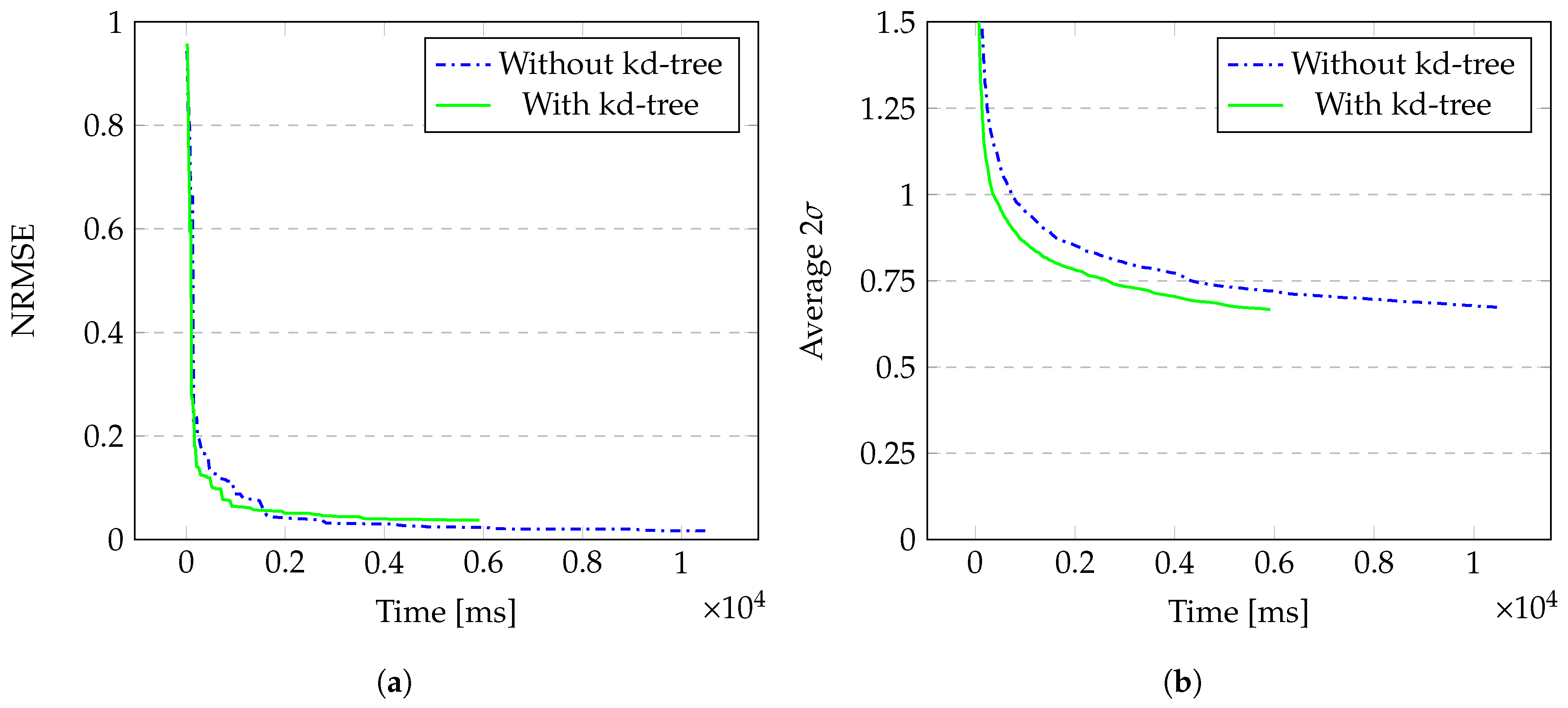
Results for the Car model as 100 data points are added sequentially. (a) NRMSE between the posteriors and the ground truth; (b) average value for all points.
Figure 6.
Results for the Car model as 100 data points are added sequentially. (a) NRMSE between the posteriors and the ground truth; (b) average value for all points.


Table 1.
Time it took to perform 100 iterations. All times are given in ms.
| Model | Without kd-Tree | With kd-Tree | % Gain |
|---|---|---|---|
| Cube | 70,596 | 44,075 | 37.6 |
| Car | 10,497 | 5914 | 43.7 |
Table 2.
NRMSE after 100 iterations.
| Model | Without kd-Tree | With kd-Tree | Difference |
|---|---|---|---|
| Cube | 0.110 | 0.168 | 0.058 |
| Car | 0.017 | 0.037 | 0.020 |
Table 3.
Average two times sigma after 100 iterations.
| Model | Without kd-Tree | With kd-Tree | Difference |
|---|---|---|---|
| Cube | 0.449 | 0.439 | 0.010 |
| Car | 0.673 | 0.666 | 0.007 |
Publisher’s Note: MDPI stays neutral with regard to jurisdictional claims in published maps and institutional affiliations. |
© 2020 by the authors. Licensee MDPI, Basel, Switzerland. This article is an open access article distributed under the terms and conditions of the Creative Commons Attribution (CC BY) license (http://creativecommons.org/licenses/by/4.0/).
Share and Cite
MDPI and ACS Style
De Boi, I.; Ribbens, B.; Jorissen, P.; Penne, R. Feasibility of Kd-Trees in Gaussian Process Regression to Partition Test Points in High Resolution Input Space. Algorithms 2020, 13, 327. https://0-doi-org.brum.beds.ac.uk/10.3390/a13120327
AMA Style
De Boi I, Ribbens B, Jorissen P, Penne R. Feasibility of Kd-Trees in Gaussian Process Regression to Partition Test Points in High Resolution Input Space. Algorithms. 2020; 13(12):327. https://0-doi-org.brum.beds.ac.uk/10.3390/a13120327
Chicago/Turabian StyleDe Boi, Ivan, Bart Ribbens, Pieter Jorissen, and Rudi Penne. 2020. "Feasibility of Kd-Trees in Gaussian Process Regression to Partition Test Points in High Resolution Input Space" Algorithms 13, no. 12: 327. https://0-doi-org.brum.beds.ac.uk/10.3390/a13120327
Note that from the first issue of 2016, this journal uses article numbers instead of page numbers. See further details here.