Improving Scalable K-Means++

Abstract

Two new initialization methods for K-means clustering are proposed. Both proposals are based on applying a divide-and-conquer approach for the K-means‖ type of an initialization strategy. The second proposal also uses multiple lower-dimensional subspaces produced by the random projection method for the initialization. The proposed methods are scalable and can be run in parallel, which make them suitable for initializing large-scale problems. In the experiments, comparison of the proposed methods to the K-means++ and K-means‖ methods is conducted using an extensive set of reference and synthetic large-scale datasets. Concerning the latter, a novel high-dimensional clustering data generation algorithm is given. The experiments show that the proposed methods compare favorably to the state-of-the-art by improving clustering accuracy and the speed of convergence. We also observe that the currently most popular K-means++ initialization behaves like the random one in the very high-dimensional cases.

1. Introduction

Clustering is one of the core techniques in data mining. Its purpose is to form groups from data in a way that the observations within one group, the cluster, are similar to each other and dissimilar to observations in other groups. Prototype-based clustering algorithms, such as the popular K-means [1], are known to be sensitive to initialization [2,3], i.e., the selection of initial prototypes. A proper set of initial prototypes can improve the clustering result and decrease the number of iterations needed for the convergence of an algorithm [3,4]. The initialization of K-means was remarkably improved by the work of Arthur and Vassilvitskii [5], where they proposed the K-means++ method. There, the initial prototypes are determined by favoring distinct prototypes, which in high probability are not similar to the already selected ones.

A drawback of K-means++ is that the initialization phase requires K inherently sequential passes over the data, since the selection of a new initial prototype depends on the previously selected prototypes. Bahmani et al. [6] proposed a parallel initialization method called K-means‖ (Scalable K-means++). The K-means‖ speeds up initialization by sampling each point independently and by updating sampling probabilities less frequently. Independent sampling of the points enables parallelization of the initialization, thus providing a speedup over K-means++. However, for example MapReduce-based implementation of K-means‖ needs multiple MapReduce jobs for the initialization. The MapReduce K-means++ method [7] tries to address this issue, as it uses one MapReduce job to select K initial prototypes, which speeds up the initialization compared to K-means‖. Suggestions of parallelizing the second, search phase of K-means have been given in several papers (see, e.g., [8,9]). On a single machine, distance pruning approaches can be used to speed up K-means without affecting the clustering results [10,11,12,13,14]. Besides parallelization and distance pruning, data summarization is also a viable option for speeding up the K-means clustering [15,16].

Dimension reduction has had an important role in making clustering algorithms more efficient. Over the years, various dimension reduction methods have been applied to decrease the dimension of data in order to speed up clustering algorithms [17,18,19,20]. The key idea for improved efficiency is to solve an approximate solution to the clustering problem in a lower-dimensional space. Dimension reduction methods are usually divided into two categories: feature selection methods and feature extraction methods [21]. Feature selection methods aim to select a subset of the most relevant variables from the original variables. Correspondingly, feature extraction methods aim to transform the original dataset into a lower-dimensional space while trying to preserve the characteristics (especially distances between the observations and the overall variability) of the original data.

A particular dimensional reduction approach for processing large datasets is the random projection (RP) method [22]. Projecting data from the original space to a lower-dimensional space while preserving the distances is the main characteristic of the RP method. This makes RP very appealing in clustering, whose core concept is dissimilarity. Moreover, classical dimension reduction methods such as the principal component analysis (PCA) [23] become expensive to compute for high-dimensional spaces whereas RP remains computationally efficient [24].

Fern and Brodley [18] proposed an ensemble clustering method based on RP. They showed empirically that aggregation of clustering results from multiple lower-dimensional spaces produced by RP leads to better clustering results compared to a single clustering in lower-dimensional space produced by PCA or RP. Other combinations of K-means and RP have been studied in several papers [17,25,26,27]. RP for K-means++ was analyzed in [28]. Generally, the main idea is to create a lower-dimensional dataset with RP and to solve the ensuing K-means clustering problem with less computational effort. On the other hand, one can also optimize clustering method’s proximity measure for small datasets [29].

In general, K-means clustering procedure typically uses a non-deterministic initialization, such as K-means++, followed by the Lloyd’s iterations [1]—with multiple restarts. Prototypes corresponding to the smallest sum-of-squares clustering error are selected as the final clustering result. In [30], such a multistart strategy was carried out during the initialization phase, thus reducing the need to repeat the whole clustering algorithm. More precisely, a parallel method based on K-means++ clustering of subsets produced by the distribution optimally balanced stratified cross-validation (DOB-SCV) algorithm [31] was proposed and tested. Here, such an approach is developed further with the help of K-means‖ and RP. More precisely, we run K-means‖ method in a low-dimensional subset created by RP. In contrast to the previous work [30], the new methods also restrict the number of Lloyd’s iterations in the subsets.

Vattani [32] showed by construction that the number of iterations, and thus the running time, of the randomly initialized K-means algorithm can grow exponentially already in small-dimensional spaces. As stated in the original papers [5,6], the K-means++ and K-means‖ readily provide improvements to this both in theory and in practice. Concerning our work, we have provided time complexity analysis for SK-means‖ in Section 3.1 and for SRPK-means‖ in Section 3.2. In terms of time complexity, SRPK-means$\left|\right|$ reduces the time complexity of the initialization for large-scale high-dimensional data (this was also confirmed by our experimental results) and provides better clustering results; thus, it reduces need for restarts compared to the baseline methods. Reduced need for restarts also improves the overall time complexity of K-means algorithm. In terms of clustering accuracy, SK-means does this same effect for large-scale lower-dimensional datasets. Moreover, we showed for the synthetic datasets (M-spheres) that the random projection variant of the initialization (SRPK-means‖) can provide clear advantage in very high-dimensional cases, where the distances can become meaningless for other distance-based initialization methods.

The main purpose of this article is to propose two new algorithms for clustering initialization and compare them experimentally to the initializations of K-means++ and K-means‖ using several large-scale datasets. To summarize the main justification of the proposed methods: they provide better results compared to baseline methods with better or equal running time. The proposed initialization method reduces data processing with sampling, subsampling, and dimensional reduction solving the K-means clustering problem in a coarse fashion. Moreover, from the perspective of parallel computing, using a parallelizable clustering method in the subset clustering allows fixing the number of subsets and treating each subset locally in parallel, hence improving the scalability.

For quantified testing and comparison of the methods, we introduce a novel clustering problem generator for high dimension spaces (see Section 3.4). Currently, challenging simulated datasets for high-dimensional clustering problems are difficult to find. For instance, the experiments with DIM datasets of tens or hundreds of dimensions in [4] were inconclusive: all clustering results and cluster validation index comparisons behaved perfectly without any errors. Therefore, better experimental datasets are needed and can be produced with the proposed algorithm.

2. Existing Algorithms

In this section, we introduce the basic composition of the existing algorithms.

2.1. K-Means Clustering Problem and the Basic Algorithms

Let $\mathbf{X}=\{{\mathbf{x}}_1,{\mathbf{x}}_2,...,{\mathbf{x}}_N\}$ be a dataset such that ${\mathbf{x}}_i\in {\mathbb{R}}^M\forall 1\le i\le N$, where M denotes the dimension, and let $\mathbf{C}=\{{\mathbf{c}}_1,{\mathbf{c}}_2,...,{\mathbf{c}}_K\}$ be a set of prototypes, where each prototype also belongs to ${\mathbb{R}}^M$. The goal of the K-means clustering algorithm is to find a partition of $\mathbf{X}$ into K disjoint subsets, by minimizing the sum-of-squares error (SSE) defined as

$$\mathrm{SSE}\left(\mathbf{C}\right)=\sum _{\mathbf{x}\in \mathbf{X}}\underset{\mathbf{c}\in \mathbf{C}}{min}{\parallel \mathbf{c}-\mathbf{x}\parallel }^2.$$

(1)

An approximate solution to the minimization problem with (1) is typically computed by using the Lloyd’s K-means algorithm [1]. Its popularity is based on simplicity and scalability. Even if the cost function in (1) is mathematically nondifferentiable because of the min-operator, it is easy to show that after the initialization, the K-means type of iterative relocation algorithm converges in finite many steps [4].

Prototype-based clustering algorithms, such as K-means, are initialized before the prototype relocation (search) phase. The classical initialization algorithm, readily proposed in [33], is to randomly generate the initial set of prototypes. A slight refinement of this strategy is to select, instead of random points (from appropriate value ranges), random indices and use the corresponding observations in data as initialization [34]. Because of this choice, there cannot be empty clusters in the first iteration. Bradley and Fayyad [35] proposed an initialization method where J randomly selected subsets of the data are first clustered with K-means. Next, it forms a superset of the $J\times K$ prototypes obtained from the subset clustering. Finally, the initial prototypes are achieved as the result of K-means clustering of the superset.

Arthur and Vassilvitskii [5] introduced the K-means++ algorithm, which improves the initialization of K-means clustering. The algorithm selects first prototype at random, and then the remaining $K-1$ prototypes are sampled using probabilities based on the squared distances to the already selected set, thus favoring distant prototypes. The generalized form of such an algorithm with different $l_p$-distance functions and the corresponding cluster location estimates was depicted in [4].

The parallelized K-means++ method, called K-means‖, was proposed by Bahmani et al. [6] (see Algorithm 1). In Algorithm 1, and from here onwards, symbol “#” denotes ’number of’. In the algorithm, sampling from $\mathbf{X}$ is conducted in a slightly different fashion compared to K-means++. More precisely, the sampling probabilities are multiplied with the over-sampling factor l and the sampling is done independently for each data point. The initial SSE for the first sampled point $\psi$ determines the number of sampling iterations. K-means‖ runs $O\left(log\right(\psi \left)\right)$ sampling iterations. For each iteration, the expected number of points is l. Hence, after $O\left(log\right(\psi \left)\right)$ iterations, the expected number of points added to $\mathbf{C}$ is $O\left(llog\right(\psi \left)\right)$. Finally, weights representing the accumulation of data around the sampled points are set and the result of the weighted clustering then provides the K initial prototypes. K-means++ can be used to cluster the weighted data (see Algorithm 1 in [36]). Selecting $r=5$ instead of $O\left(log\right(\psi \left)\right)$ rounds and setting the over-sampling factor to $2K$ were demonstrated to be sufficient in [6]. Recently, Bachem et al. [36] proved theoretically that small r instead of $O\left(log\right(\psi \left)\right)$ iterations is sufficient in K-means‖. A modification of K-means‖ for initializing robust clustering was described and tested in [37].

Algorithm 1: K-means‖

Input: Dataset $\mathbf{X}$, #clusters K, and over-sampling factor l. Output: Set of prototypes $\mathbf{C}=\{{\mathbf{c}}_1,{\mathbf{c}}_2,...,{\mathbf{c}}_K\}$.       1: $\mathbf{C}\leftarrow$ select point ${\mathbf{c}}_1$ uniformly random from $\mathbf{X}$.       2: $\psi \leftarrow$ compute $SSE\left(\mathbf{C}\right)$.       3: for $O(log(\psi \left)\right)$ times do       4:     ${\mathbf{C}}^{\prime }\leftarrow$ sample each point $\mathbf{x}\in \mathbf{X}$ independently with probability $l·{d\left(\mathbf{x}\right)}^2/SSE\left(\mathbf{C}\right)$.       5:     $\mathbf{C}\leftarrow \mathbf{C}\cup {\mathbf{C}}^{\prime }$       6: For each $\mathbf{x}$ in $\mathbf{C}$ attach a weight defined as the number of points in $\mathbf{X}$ closer to $\mathbf{x}$ than any other point in $\mathbf{C}$.       7: Do a weighted clustering of $\mathbf{C}$ into K clusters.

2.2. Random Projection

The background for RP [22] comes from the Johnson–Lindenstrauss lemma [38]. The lemma states that points in a high-dimensional space can be projected to a lower dimension space while approximately preserving the distances of the points, when the projection is done with a matrix whose elements are randomly generated. Hence, for an $N\times M$ dataset $\mathbf{X}$, let $\mathbf{R}\in M\times P$ be a random matrix. Then, the random projected data matrix $\tilde{\mathbf{X}}$ is given by $\tilde{\mathbf{X}}=\frac{1}{\sqrt{P}}\mathbf{X}\mathbf{R}.$ The random matrix $\mathbf{R}$ consists of independent random elements $\left(r_{ij}\right)$ which can be drawn from one of the following probability distributions [22]: $r_{ij}=+1$ with probability $1/2$, or $-1$ with probability $1/2$; or $r_{ij}=+1$ with probability $1/6$, 0 with probability $2/3$, or $-1$ with probability $1/6$.

3. New Algorithms

Next we introduce the novel initialization algorithms for K-means, their parallel implementations, and the novel dataset generator algorithm.

3.1. SK-Means‖

The first new initialization method for K-means clustering, Subset K-means‖ (SK-means‖), is described in Algorithm 2. The method is based on S randomly sampled non-disjoint subsets $\{{\mathbf{X}}_1,{\mathbf{X}}_2,...,{\mathbf{X}}_S\}$ from $\mathbf{X}$ of approximately equal size, such as $\mathbf{X}={\cup }_{i=1}^S{\mathbf{X}}_i$. First, K-means‖ is applied in each subset, which gives the corresponding set of initial prototypes ${\mathbf{C}}_i$. Next, each initial prototype set ${\mathbf{C}}_i$ in ${\mathbf{X}}_i$ is refined with $T_{init}$ Lloyd’s iterations. $T_{init}$ is assumed to be significantly smaller than the number of Lloyd’s iterations needed for convergence. Then, SSE is computed locally for each ${\mathbf{C}}_i$ in ${\mathbf{X}}_i$. Differently from the earlier work [30], this locally computed SSE is now used as the selection criteria for the initial prototypes instead of the global SSE. Computation of SSE for ${\mathbf{X}}_i$ in Step 3 is obviously much faster than to compute it for the whole $\mathbf{X}$. However, a drawback is that if the subsets are too small to characterize the whole data, the selection of the initial prototypes might fail. Therefore, S should be selected such that the subsets are sufficiently large. For example, if S is close to the number of samples in the smallest cluster, then this cluster will appear as an anomaly for most of the subsets. On the other hand, this property can also be beneficial to exclude anomalous clusters already in the initialization phase. Currently, there are no systematic comparisons in the literature on the size of the subsets in sampling-based clustering approaches [39]. In [35], the number of subsets was set to 10. Based on [30,35], this selection appears reasonable for the sampling-based clustering initialization approaches.

Algorithm 2: SK-means‖

Input: Subsets $\{{\mathbf{X}}_1,{\mathbf{X}}_2,...,{\mathbf{X}}_S\}$, #clusters K, and #Lloyd’s iterations $T_{init}$. Output: Set of prototypes $\mathbf{C}=\{{\mathbf{c}}_1,{\mathbf{c}}_2,...,{\mathbf{c}}_K\}$.       1: ${\mathbf{C}}_i\leftarrow$ for each subset ${\mathbf{X}}_i$ run K-means‖.       2: ${\mathbf{C}}_i\leftarrow$ for each subset ${\mathbf{X}}_i$ run $T_{init}$ Lloyd’s iterations initialized with ${\mathbf{C}}_i$.       3: Compute local SSE for each ${\mathbf{C}}_i$ in ${\mathbf{X}}_i$.       4: $\mathbf{C}\leftarrow$ select prototypes corresponding to smallest local SSE.

The convergence rate of K-means is fast and the most significant improvements in the clustering error are achieved during the first few iterations [40,41]. Therefore, for the initialization purposes, $T_{init}$ can restricted, e.g., to 5 iterations. Moreover, since the number of Lloyd’s iterations needed for convergence might vary significantly (e.g., [4]), a restriction on the number of Lloyd’s iterations helps in synchronization, when a parallel implementation of the SK-means‖ method is used.

The computational complexity of the K-means‖ method is of the order $\mathcal{O}\left(rlNM\right)$, where r is the number of initialization rounds. Therefore, SK-means‖ also has the complexity of the order $\mathcal{O}\left(rlNM\right)$ in Step 1. In addition, SK-means‖ runs $T_{init}$ Lloyd’s iterations with the complexity of $\mathcal{O}\left(T_{init}KNM\right)$, and computes local SSE with the complexity of $\mathcal{O}\left(KNM\right)$. Hence, the total complexity of SK-means‖ is of the order $\mathcal{O}(rlNM+T_{init}KNM)$.

3.2. SRPK-Means‖

The second novel proposal, Subset Random Projection K-means‖ (SRPK-means‖), adds RPs to SK-means‖. Since SK-means‖ mainly uses time in computing distances in Steps 1 and 2, it is reasonable to speed up the distance computation with RP. The RP-based method is presented in Algorithm 3. Generally, SRPK-means‖ computes a set of candidate initial prototypes in a lower-dimensional space and then evaluates these in the original space. As with Algorithm 2, the best set of prototypes based on the local SSE are selected.

Algorithm 3: SRPK-means‖

Input: Subsets $\{{\mathbf{X}}_1,{\mathbf{X}}_2,...,{\mathbf{X}}_S\}$, #clusters K, #Lloyd’s iterations $T_{init}$, and random projection dimension P. Output: Set of prototypes $\mathbf{C}=\{{\mathbf{c}}_1,{\mathbf{c}}_2,...,{\mathbf{c}}_K\}$.       1: ${\mathbf{R}}_i\leftarrow$ for each subset ${\mathbf{X}}_i$ generate $M\times P$ random matrix.       2: ${\tilde{\mathbf{X}}}_i\leftarrow$ for each subset ${\mathbf{X}}_i$ compute $\frac{1}{\sqrt{P}}{\mathbf{X}}_i{\mathbf{R}}_i$       3: ${\tilde{\mathbf{C}}}_i\leftarrow$ for each ${\tilde{\mathbf{X}}}_i$ run K-means‖.       4: ${\mathbf{I}}_i\leftarrow$ for each ${\tilde{\mathbf{X}}}_i$ run $T_{init}$ Lloyd’s iterations initialized with ${\tilde{\mathbf{C}}}_i$.       5: For each partitioning ${\mathbf{I}}_i$ compute prototypes ${\mathbf{C}}_i$ in original space ${\mathbf{X}}_i$.       6: Compute local SSE for each ${\mathbf{C}}_i$ in ${\mathbf{X}}_i$.       7: $\mathbf{C}\leftarrow$ select prototypes corresponding to smallest local SSE.

The proposal first computes a unique random matrix for each subset ${\mathbf{X}}_i$. Then, the P-dimensional random projected subset ${\tilde{\mathbf{X}}}_i$ is computed in each subset ${\mathbf{X}}_i$. Steps 3–4 are otherwise the same as the Steps 1–2 in Algorithm 2, but these steps are applied for the lower-dimensional subsets $\{{\tilde{\mathbf{X}}}_1,{\tilde{\mathbf{X}}}_2,...,{\tilde{\mathbf{X}}}_S\}$. Next, the labels ${\mathbf{I}}_i$ for partitioning each subset are used to compute ${\mathbf{C}}_i$ in the original space ${\mathbf{X}}_i$. Finally, the local SSEs are computed, and the best set of prototypes are returned as the initial prototypes. Please note that the last two steps in Algorithm 3 are the same as Steps 3–4 in Algorithm 2. SRPK-means‖ computes projected data matrices, which require a complexity of $\mathcal{O}\left(PNM\right)$ (naive multiplication) [17]. Execution of K-means‖ in the lower-dimensional space requires $\mathcal{O}\left(rlNP\right)$, and $T_{init}$ Lloyd’s iterations requires $\mathcal{O}\left(T_{init}KNP\right)$ operations. Step 6 requires $\mathcal{O}\left(KNM\right)$ operations, since it computes the local SSEs in the original space, so that the total computational complexity of the SRPK-means‖ method is $\mathcal{O}(PNM+rlNP+T_{init}KNP+KNM)$. Typically, applications of RP are based on the assumption $P<<M$. Thus, when the dimension of data M is increased, the contribution of the second and the third term of the total computational complexity start to diminish. Moreover, when both M and K are large compared to P, the last term dominates the overall computational complexity. Therefore, in terms of running time, SRPK-means‖ is especially suited for clustering large-scale data with very high dimensionality into a large number of clusters.

Fern and Brodley [18] noted that clustering with RP produces highly unstable and diverse clustering results. However, this can be exploited in clustering to find different candidate structures of data, which then can be combined into a single result [18]. The proposed initialization method in this paper uses a similar idea as it tries to find structures from multiple lower-dimensional spaces that minimize the local SSE. In addition, selecting a result that gives the smallest local SSE excludes the bad structures, which could be caused by inappropriate ${\mathbf{R}}_i$ or ${\mathbf{C}}_i$.

3.3. Parallel Implementation of the Proposed K-Means Initialization Algorithms

Bahmani et al. [6] implemented K-means‖ with the MapReduce programming model. It can also be implemented by the Single Program Multiple Data (SPMD) programming model with message passing. Then all the steps of the parallelized Algorithms 1–3 are executed inside an SPMD block. Next, a parallel implementation of K-means‖ as depicted in Algorithm 1 is briefly described, by using Matlab Parallel Computing Toolbox (PCT), SPMD blocks, and message passing functions (see [42] for a detailed description about PCT). First, data $\mathbf{X}$ is split into Q subsets of approximately equal size and then the subsets are distributed to Q workers. Step 1 picks a random point from a random worker and broadcasts this point to all other workers. In Step 2, each worker calculates distances and SSE for its local data. Next, points are aggregated by calling gplus-function, after which the aggregation distributes this sum to other workers. In Steps 4 and 5, each worker samples points from its local data, the next points are aggregated to ${\mathbf{C}}^{\prime }$ by calling gop-function, and then ${\mathbf{C}}^{\prime }$ is broadcasted to all workers. Again, distances and SSE are calculated similarly as in Step 2. Each worker in Step 6 assigns weights based on its local data, after which the weights are aggregated with gop-function. Finally, Step 7 is computed sequentially.

As with the parallel K-means‖ implementation, a parallel implementation of Algorithm 2 with SMPD and message passing is described next. First, each subset ${\mathbf{X}}_i$ from S subsets is split into J approximately equal size subsets and then these subsets are distributed to $J\times S$ workers, e.g., subset ${\mathbf{X}}_i$ is distributed to workers $(i-1)J+1,...,(i-1)J+J$. In Steps 1–3, each subset of workers runs steps for subset ${\mathbf{X}}_i$ in parallel similarly as described in the previous paragraph. For parallel Lloyd’s iterations, a similar strategy as proposed in [8] can be used in Step 2. Steps 1–3 require calling modified gop-function and gplus-function for the subset of workers; these functions were modified to support this requirement. Finally, prototypes corresponding to the smallest local SSE from the subset $i^{\prime }$ allocated workers $(i^{\prime }-1)J+1,...,(i^{\prime }-1)J+J$ are returned as the initialization.

The parallel SRPK-means‖ in Algorithm 3 can be implemented in a highly similar fashion to the parallel SK-means‖. More precisely, in Step 1, each worker $(i-1)J+1$, where $i\in \{1,2,...,S\}$, generates the random matrix ${\mathbf{R}}_i$ and broadcasts it to workers $(i-1)J+1,...,(i-1)J+J$. In Step 2, each worker computes random projected data for its local data. Steps 3–4 are otherwise computed similarly to the parallel SK-means‖ Steps 1 and 2, except these steps are executed for the projected subsets. In Step 5, the prototypes are computed in the original space in parallel. Finally, Steps 6 and 7 are the same as Steps 3 and 4 in Algorithm 2. The parallel implementations of the proposed methods and K-means‖ are available in (https://github.com/jookriha/Scalable-K-means).

3.4. M-Spheres Dataset Generator

The novel dataset generator is given in Algorithm 4. Based on the method proposed in ([43], p. 586), Algorithm 5 generates a random point that is on the M-dimensional sphere centered on $\mathbf{c}$ with radius of d. The core principle is to draw M independent values from the standard normal distribution and transform these with corresponding M-direction cosines. The obtained M-dimensional vector is then scaled with the radius d and relocated with the center $\mathbf{c}$. The generated points are uniformly distributed on the surface of the sphere, because of the known properties of the standard normal distribution (see [43] (p. 587) and articles therein).

Algorithm 4:M-spheres dataset generator.

Input: #clusters K, #dimensions M, #points per cluster $N_K$, nearest center distance $d_c$, radius of M-sphere $d_r$. Output: Dataset $\mathbf{X}=\{{\mathbf{x}}_1,{\mathbf{x}}_2,...,{\mathbf{x}}_N\}$.       1: $\mathbf{C}\leftarrow$ {(0,...,0)}.       2: if $K>1$ then       3:      ${\mathbf{c}}_2\leftarrow$ randsurfpoint(${\mathbf{c}}_1$,$d_c$).       4:     $\mathbf{C}\leftarrow$$\mathbf{C}\cup \left\{{\mathbf{c}}_2\right\}$.       5:     $k\leftarrow 2$.       6: if $K>2$then       7:     while $k<K$ do       8:         $i\leftarrow$ rand($\{1,2,...,k\}$).       9:         ${\mathbf{c}}_{cand}\leftarrow$ randsurfpoint(${\mathbf{c}}_i$,$d_c$).       10:         $i^{*}\leftarrow {argmin}_j\parallel {\mathbf{c}}_j-{\mathbf{c}}_{cand}\parallel$.       11:         if $i^{*}==i$ then       12:            $\mathbf{C}\leftarrow$$\mathbf{C}\cup \left\{{\mathbf{c}}_{cand}\right\}$.       13:            $k\leftarrow k+1$.       14: $k\leftarrow 1$.       15: $\mathbf{X}\leftarrow \left\{\right\}$.       16: while$k\le K$do       17:     $n\leftarrow 1$       18:     while $n\le N_K$ do       19:         $d_r^{*}\leftarrow rand\left((0,d_r]\right)$       20:         ${\mathbf{x}}_{new}\leftarrow$ randsurfpoint(${\mathbf{c}}_k$,$d_r^{*}$).       21:         $\mathbf{X}\leftarrow \mathbf{X}\cup \left\{{\mathbf{x}}_{new}\right\}$.       22:         $n\leftarrow n+1$       23:     $k\leftarrow k+1$

The generator uses Algorithm 5 for generating K cluster centers so that $\parallel {\mathbf{c}}_i-{\mathbf{c}}_j\parallel =d_c$, where $i\ne j$, $d_c$ is the given distance between the centers, and both ${\mathbf{c}}_i,{\mathbf{c}}_j$ then belong to the set of centers $\mathbf{C}$. Finally, $N_K$ data points for each cluster are generated by applying Algorithm 5 with a uniformly random radius from the interval $(0,d_r]$. This means, in particular, that points in a cluster are nonuniformly distributed and approximately $\frac{100a}{d_r}\%$ percentages of the points are within a M-dimensional sphere with radius a for $0\le a\le d_r$. In Algorithm 5, $\mathcal{N}(0,1)$ denotes the standard normal distribution.

Algorithm 5: randsurfpoint($\mathbf{c}$,d).

Input: Sphere center $\mathbf{c}$, sphere radius d. Output: New point ${\mathbf{x}}^{*}$.       1: $m\leftarrow 1$.       2: $S\leftarrow 0$.       3: while$m\le M$do       4:     $x_m\leftarrow \mathcal{N}(0,1)$.       5:     $S\leftarrow S+x_m^2$.       6:     $m\leftarrow m+1$.       7: ${\mathbf{x}}^{*}\leftarrow \mathbf{c}+d{S}^{-1/2}\mathbf{x}$

For simplicity, generation of the cluster centers starts from the origin. When the new centers are randomly located with the fixed distance and then expanded as clusterwise data in ${\mathbb{R}}^M$, the generator algorithm does not restrict the actual values of the generated data and centers. Hence, depending on the input, data range can be large. However, this can be alleviated with the min-max scaling as part of the clustering process.

4. Empirical Evaluation of Proposed Algorithms

In this section, empirical comparison between K-means++, K-means‖, SK-means‖, and SRPK-means‖ is presented by using 21 datasets. In Section 4.1, the results are given for 15 reference datasets. The performance of the methods was evaluated by analyzing SSE, the number of iterations needed for convergence, and the running time. Finally, In Section 4.2, we analyze the final clustering accuracy for six novel synthetic datasets that highlight the effects of the curse of dimensionality in the K-means++ type initialization strategies. The simulated clustering problems have been formed with the novel generator described in Algorithm 4. The MATLAB implementation of the algorithm is available in (https://github.com/jookriha/M_Spheres_Dataset_Generator).

4.1. Experiments with Reference Datasets

In this section, the results are shown and analyzed for 15 publicly available reference datasets by considering separately the accuracy (Section 4.1.2), efficiency (Section 4.1.3), and scalability (Section 4.1.4) of the algorithms.

4.1.1. Experimental Setup

Basic information about the datasets is shown in

Table 1. Characteristics of datasets. The number of clusters K was chosen according to the known number of classes or fixed by hand. The latter choice is indicated with symbol *.

Dataset	#Observations (N)	#Features (M)	#Clusters (K)
HAR	7352	561	6
ISO	7797	617	26
LET	20,000	16	26
GFE	27,936	300	36
MNI	70,000	784	10
BIR	100,000	2	100
BSM	583,250	77	50 *
FCT	581,012	54	7
SVH	630,420	3072	100 *
RCV	781,265	1000	350
USC	2,458,285	68	100 *
KDD	4,898,431	41	100 *
M8M	8,100,000	784	265
TIN	15,860,403	384	100 *
OXB	16,334,970	128	100 *

. The parallel implementations of the proposed methods and K-means‖ (omitting K-means++ readily tested in [6]) were applied to the seven largest datasets and serial implementations were used otherwise. For the serial experiments, we used the following eight datasets: Human Activity Recognition Using Smartphones (http://archive.ics.uci.edu/ml/index.php) (HAR), ISOLET (ISO), Letter Recognition (LET), Grammatical Facial Expressions (GFE), MNIST (http://yann.lecun.com/exdb/mnist/) (MNI), Birch3 (http://cs.joensuu.fi/sipu/datasets/) (BIR), Buzz in Social Media (BSM), and Covertype (COV). For the parallel experiments, the following seven large high-dimensional datasets were used: KDD Cup 1999 Data (KDD), US Census Data 1990 (USC), Oxford Buildings (http://www.robots.ox.ac.uk/~vgg/data/oxbuildings/) (OXB), Tiny Images (http://horatio.cs.nyu.edu/mit/tiny/data/) (TIN), MNIST8M (M8M), RCV1v2 collection of documents (https://www.csie.ntu.edu.tw/~cjlin/libsvmtools/datasets) (RCV) and Street View House Numbers (http://ufldl.stanford.edu/housenumbers/) (SVH). The BIR dataset [44] was selected to test SK-means‖ for low-dimensional data. With the OXB dataset, we used the transformed dataset with 128-dimensional SIFT descriptors extracted from the original dataset. For the TIN dataset, we sampled a 20% subset from the Gist binary file (tinygist80million.bin), where 79,302,017 images are characterized with 384-dimensional Gist descriptors. The highest-dimensional dataset was SVH, where we combined the training, testing, and validation subsets into a single dataset. We excluded the attack type feature (class label) from the KDD dataset, used the Twitter data for the BSM dataset, and restricted to the training dataset of the HAR dataset. For the RCV dataset, we used the full industries test set (350 categories) and selected 1000 out 47,236 features with the same procedure as in [45]. For the M8M and the RCV datasets, we used the scaled datasets given in http://cs.joensuu.fi/sipu/datasets/, all other datasets were min-max scaled into $[-1,1]$.

In Section 3.1, we discussed the selection of parameter S. Because the results in [30,35] and that the computing nodes’ have typically the number of cores in powers of two, we fixed $S=8$ in the experiments. This means that each dataset was randomly divided into 8 subsets, which were roughly of equal size. Matlab 2018a environment was used in the serial experiments with the K-means$++$, K-means‖, SK-means‖ and SRPK-means‖ methods. In Matlab 2018a version, we were not able to modify gop-function and gplus-function (see Section 3.3). In Matlab R2014a environment, these modifications were possible for the proposed methods. To follow the good practices of running time evaluation [46], all the parallel experiments with the K-means‖, SK-means‖ and SRPK-means‖ methods were run Matlab R2014a environment. The parallel algorithms were implemented with Matlab Parallel Computing Toolbox with the SPMD blocks and message passing functions as discussed in Section 3.3. The parallel experiments were run in a computer cluster using Sandy Bridge nodes with 16 cores and 256 GB memory. A parallel pool of 32 workers was used in the experiments; therefore, 4 workers were allocated for each subset. In the parallel experiments, each worker had a $\frac{1}{4}$ random disjoint partition of the subset on the local workspace.

For all datasets we used the following settings: (i) for K-means‖: $l=2K$ and $r=5$; (ii) for SK-means‖ and SRPK-means‖: $T_{init}=5$ and $S=8$; (iii) and for SRPK-means‖: $P\in \{5,10,20,40\}$ and R with $r_{ij}=\pm 1$. Please note that occurrence of an empty cluster for SRPK-means‖ is possible in rare cases when all S subsets produce an empty cluster. (For instance, empty clusters appeared seven times in all the experiments with the synthetic datasets as reported in Section 4.2). In these cases, we repeated the whole clustering initialization from the start. After initialization, the Lloyd’s algorithm was executed until the number of new assignments between the consecutive iterations was below or equal to the threshold. For the five largest datasets (SVH, RCV, OXB, M8M and TIN) we set this threshold to $1\%$ of N and otherwise to zero. In the parallel experiments, runs were repeated 10 times for each setting. In the serial experiments, runs were repeated 100 times for each setting. Values for the number of clusters, K, are given in the last column of Table 1. Since the MNIST8M dataset is constructed artificially from the original MNIST dataset, we set K for MNIST8M based on the optimal value for MNIST used by Gallego et al. [47]. Otherwise, the selection is either based on the known number of classes or fixed arbitrarily (indicated with * in Table 1).

The quality of the clustering results between the methods was compared by using SSE. The SSE values were computed with formula (1) for the whole data. Finally, statistical comparison between the methods was performed with the nonparametric Kruskal-Wallis test [48,49], since in most cases the clustering errors were not normally distributed. The significance level was set to $0.05$.

4.1.2. Results for Clustering Accuracy

SSE values after the initialization (initial SSE) and after the Lloyd’s iterations (final SSE) are summarized in

Table 2. Clustering accuracy using SSE. The statistically significant differences of the final SSE according to the Kruskal-Wallis test are indicated with $**$ in the first column. Symbols +, *, ‡, and ${†}_{P^{\prime }}$ indicate that the method has statistically significantly better SSE in a pairwise comparison with respect to K-means++ (K$++$), K-means‖ (K‖), SK-means‖ (SK‖), and SRPK-means‖ (SRPK‖) for $P=P^{\prime }$, respectively. The coefficient under the name of the data in the first column is the data-specific multiplier which scales the SSE to the true level. The best performances are highlighted in bold.

		Initialization							Final
		K$++$	K‖	SK‖	SRPK‖				K$++$	K‖	SK‖	SRPK‖
Data	Stats				$\mathit{p}=5$	$\mathit{p}=10$	$\mathit{p}=20$	$\mathit{p}=40$				$\mathit{p}=5$	$\mathit{p}=10$	$\mathit{p}=20$	$\mathit{p}=40$
HAR ${}^{**}$	median	2.5881	1.5577	1.3958	1.4474	1.4192	1.4074	1.4003	1.3803	1.3803	1.3707 ${}^{+,*}$	1.3707 ${}^{+,*}$	1.3707 ${}^{+,*}$	1.3707 ${}^{+,*}$	1.3707 ${}^{+,*}$
${10}^5$	mad	0.1498	0.0436	0.0066	0.0250	0.0175	0.0132	0.0116	0.0203	0.0242	0.0057	0.0117	0.0087	0.0082	0.0064
	max	3.2295	1.7367	1.4316	1.5269	1.4613	1.4504	1.4621	1.5461	1.5461	1.4126	1.4136	1.4110	1.4126	1.4094
	min	2.2533	1.4782	1.3785	1.3971	1.3907	1.3859	1.3825	1.3707	1.3707	1.3707	1.3707	1.3707	1.3707	1.3707
ISO ${}^{**}$	median	8.9267	5.5274	4.9617	5.7887	5.4478	5.198	5.0575	4.7811	4.7795	4.7617 ${}^{+,*}$	4.7578 ${}^{+,*}$	4.7558 ${}^{+,*}$	4.7538 ${}^{+,*}$	4.7575 ${}^{+,*}$
${10}^5$	mad	0.1797	0.0575	0.0271	0.0927	0.0723	0.0486	0.0411	0.0287	0.0246	0.0202	0.0277	0.0306	0.0265	0.0267
	max	9.4413	5.7650	5.0490	6.0687	5.6078	5.2900	5.1494	4.9228	4.8663	4.8529	4.8469	4.8824	4.8407	4.8787
	min	8.4326	5.3859	4.8820	5.6207	5.2543	5.0629	4.9383	4.7142	4.7085	4.7087	4.7145	4.7099	4.7084	4.7180
LET ${}^{**}$	median	1.7868	1.2356	1.1415	1.3543	1.2339	-	-	1.1012	1.1014	1.0985 ${}^{*}$	1.0994	1.0989	-	-
${10}^4$	mad	0.0517	0.0176	0.0070	0.0372	0.0217	-	-	0.0062	0.0060	0.0051	0.0064	0.0065	-	-
	max	2.1162	1.3133	1.1616	1.4327	1.2991	-	-	1.1261	1.1192	1.1218	1.1175	1.1219	-	-
	min	1.6656	1.1771	1.1175	1.2617	1.1844	-	-	1.0872	1.0873	1.0883	1.0876	1.0875	-	-
GFE ${}^{**}$	median	3.0103	2.0860	1.9218	2.1637	2.0463	1.9813	1.9506	1.8605	1.8550	1.8491 ${}^{+}$	1.8398 ${}^{+,*,‡}$	1.8397 ${}^{+,*,‡}$	1.8407 ${}^{+,*,‡}$	1.8420 ${}^{+,*,‡}$
${10}^5$	mad	0.0994	0.0231	0.0155	0.0415	0.0258	0.0727	0.0704	0.0151	0.0146	0.0117	0.0129	0.0123	0.0119	0.0113
	max	3.3933	2.1737	1.9793	2.2439	2.1042	2.0302	1.9990	1.9440	1.9105	1.8999	1.8783	1.8700	1.8757	1.8771
	min	2.7908	2.0247	1.8819	2.0618	1.9802	1.9424	1.9039	1.8252	1.8197	1.8236	1.8172	1.8211	1.8227	1.8195
MNI ${}^{**}$	median	1.9539	1.2495	1.1074	1.2156	1.1752	1.1458	1.1279	1.1013	1.1013	1.0979 ${}^{+,*}$	1.0980 ${}^{+}$	1.0979 ${}^{+,*}$	1.0979 ${}^{+}$	1.0980
${10}^7$	mad	0.0624	0.0152	0.0032	0.0117	0.0093	0.0068	0.0048	0.0027	0.0024	0.0017	0.0023	0.0018	0.0026	0.0027
	max	2.2474	1.3056	1.1171	1.2428	1.1968	1.1606	1.1390	1.1146	1.1075	1.1052	1.1046	1.1069	1.1105	1.1095
	min	1.8138	1.2131	1.1006	1.1885	1.1472	1.1296	1.1136	1.0977	1.0977	1.0977	1.0977	1.0977	1.0977	1.0977
BIR ${}^{**}$	median	3.0658	1.9912	1.8677	-	-	-	-	1.8440	1.8187	1.7781 ${}^{+,*}$	-	-	-	-
${10}^2$	mad	0.1375	0.0544	0.0269	-	-	-	-	0.0469	0.0451	0.0261	-	-	-	-
	max	3.4694	2.3346	1.9533	-	-	-	-	2.0238	2.0943	1.8973	-	-	-	-
	min	2.6292	1.8770	1.8074	-	-	-	-	1.7438	1.7409	1.7248	-	-	-	-
BSM ${}^{**}$	median	1.9621	1.1802	1.0780	1.4680	1.1957	1.1038	1.1012	1.1914 ${}^{†{,}_5}$	1.1631${}^{{†}_5}$	1.0698 ${}^{+,*,{†}_{5,10}}$	1.2124	1.1324 ${}^{+,†{,}_5}$	1.0800 ${}^{+,*,†{,}_{5,10}}$	1.0903 ${}^{+,*,†{,}_{5,10}}$
${10}^5$	mad	0.1943	0.0741	0.0376	0.1593	0.0779	0.0511	0.0564	0.0818	0.0684	0.0374	0.1006	0.0741	0.0504	0.0577
	max	2.5054	1.4593	1.1776	1.8995	1.4179	1.2237	1.2130	1.4205	1.4553	1.1684	1.5541	1.2875	1.1813	1.2063
	min	1.5003	0.9999	0.9908	1.1971	0.9996	0.9779	0.9780	0.9929	0.9616	0.9739	1.0283	0.9668	0.9706	0.9664
FCT ${}^{**}$	median	3.8766	2.2187	1.9273	2.2076	2.1004	2.0086	1.9773	1.9801	2.0000	1.9132${}^{+,*,†{,}_{5-40}}$	1.9781	1.9670 ${}^{*}$	1.9461 ${}^{+,*,†{,}_5}$	1.9385${}^{+*{†}_{5,10}}$
${10}^6$	mad	0.3322	0.1013	0.0343	0.0654	0.0581	0.0508	0.0380	0.0634	0.0784	0.0354	0.0542	0.0506	0.0466	0.0435
	max	5.5290	2.5274	2.0294	2.4008	2.2494	2.1397	2.0698	2.2457	2.3487	2.0293	2.1752	2.1434	2.0852	2.0601
	min	3.1329	1.9329	1.8645	2.0808	2.0013	1.8657	1.8652	1.8644	1.8644	1.8644	1.8644	1.8644	1.8644	1.8644
SVH	median	-	1.3559	1.0855	1.1820	1.1464	1.1155	1.0992	-	1.0703	1.0704	1.0704	1.0705	1.0706	1.0708
${10}^8$	mad	-	0.0636	0.0014	0.0185	0.0149	0.0075	0.0042	-	0.0003	0.0004	0.0005	0.0005	0.0003	0.0003
	max	-	1.5968	1.0889	1.2279	1.1765	1.1290	1.1083	-	1.0711	1.0720	1.0711	1.0717	1.0714	1.0712
	min	-	1.3027	1.0836	1.1639	1.1246	1.1082	1.0922	-	1.0696	1.0698	1.0698	1.0700	1.0703	1.0703
RCV ${}^{**}$	median	-	2.5506	2.1405	2.5897	2.4864	2.3575	2.2313	-	2.0876	2.0913	2.0780	2.0757 ${}^{*,‡}$	2.0702 ${}^{*,‡,†{,}_5}$	2.0715 ${}^{*,‡,†{,}_5}$
${10}^5$	mad	-	0.0233	0.0022	0.0138	0.0041	0.0045	0.0040	-	0.0027	0.0018	0.0019	0.0014	0.0026	0.0022
	max	-	2.5886	2.1427	2.5979	2.4945	2.3652	2.2363	-	2.0922	2.0951	2.0823	2.0778	2.0767	2.0755
	min	-	2.4849	2.1345	2.5647	2.4830	2.3523	2.2228	-	2.0812	2.0863	2.0764	2.0737	2.0688	2.0674
		Initialization							Final
		K$++$	K‖	SK‖	SRPK‖				K++	K‖	SK‖	SRPK‖
Data	Stats				$\mathit{p}=\mathbf{5}$	$\mathit{p}=\mathbf{10}$	$\mathit{p}=\mathbf{20}$	$\mathit{p}=\mathbf{40}$				$\mathit{p}=\mathbf{5}$	$\mathit{p}=\mathbf{10}$	$\mathit{p}=\mathbf{20}$	$\mathit{p}=\mathbf{40}$
USC ${}^{**}$	median	-	1.7014	1.1936	1.5530	1.3218	1.2284	1.1989	-	1.1903	1.1779	1.1736 ${}^{*}$	1.1688 ${}^{*}$	1.1718 ${}^{*}$	1.1709 ${}^{*}$
${10}^7$	mad	-	0.0394	0.0036	0.0338	0.0217	0.0079	0.0037	-	0.0070	0.0057	0.0072	0.0091	0.0091	0.0049
	max	-	1.7671	1.2016	1.6178	1.3542	1.2415	1.2038	-	1.2020	1.1908	1.1803	1.1841	1.1869	1.1829
	min	-	1.6110	1.1877	1.4957	1.2799	1.2191	1.1934	-	1.1781	1.1712	1.1595	1.1566	1.1602	1.1667
KDD ${}^{**}$	median	-	30.5335	2.5466	3.1781	2.6651	2.5817	2.5162	-	2.5218	2.4726	2.4853	2.4582${}^{*}$	2.4755	2.4529 ${}^{*}$
${10}^5$	mad	-	7.3666	0.0337	0.1019	0.0483	0.0562	0.0440	-	0.0372	0.0419	0.0698	0.0413	0.0464	0.0316
	max	-	58.0452	2.5962	3.3024	2.7083	2.6275	2.6367	-	2.6288	2.5432	2.6241	2.5223	2.5640	2.5406
	min	-	22.2667	2.4803	2.9935	2.5447	2.4483	2.4878	-	2.4614	2.4084	2.3961	2.3927	2.4032	2.4330
M8M ${}^{**}$	median	-	2.6631	2.2390	2.9313	2.6415	2.4185	2.3153	-	2.2159	2.2154	2.2139 ${}^{*}$	2.2139 ${}^{*}$	2.2141 ${}^{*}$	2.2139 ${}^{*}$
${10}^8$	mad	-	0.0164	0.0009	0.0286	0.0150	0.0071	0.0041	-	0.0012	0.0008	0.0010	0.0009	0.0005	0.0009
	max	-	2.6959	2.2412	2.9835	2.6690	2.4299	2.3176	-	2.2203	2.2165	2.2162	2.2155	2.2145	2.2157
	min	-	2.6391	2.2376	2.8782	2.6192	2.4091	2.3043	-	2.2143	2.2131	2.2128	2.2126	2.2131	2.2132
TIN	median	-	10.7568	8.8782	9.7335	9.4194	9.2042	9.0595	-	8.8060	8.8065	8.8058	8.8075	8.8073	8.8073
${10}^7$	mad	-	0.1498	0.0057	0.1054	0.0879	0.0338	0.0139	-	0.0012	0.0014	0.0016	0.0018	0.0016	0.0030
	max	-	11.1649	8.8812	9.9343	9.5627	9.2543	9.0841	-	8.8091	8.8077	8.8091	8.8106	8.8093	8.8108
	min	-	10.4721	8.8623	9.5824	9.3339	9.1431	9.0474	-	8.8031	8.8029	8.8042	8.8047	8.8044	8.8024
OXB ${}^{**}$	median	-	1.7678	1.5375	1.6432	1.6249	1.6014	1.5829	-	1.5267	1.5268	1.5254 ${}^{*,‡}$	1.5256 ${}^{*,‡}$	1.5255 ${}^{*‡}$	1.5255 ${}^{*,‡}$
${10}^8$	mad	-	0.0181	0.0004	0.0055	0.0058	0.0028	0.0017	-	0.0006	0.0002	0.0003	0.0005	0.0005	0.0004
	max	-	1.8224	1.5384	1.6575	1.6315	1.6082	1.5850	-	1.5286	1.5271	1.5258	1.5266	1.5262	1.5261
	min	-	1.7506	1.5367	1.6393	1.6162	1.5995	1.5797	-	1.5258	1.5259	1.5251	1.5250	1.5250	1.5250

. For the initial SSE, we did not include any results from the statistical testing because of differences in variances. Moreover, note that the assumption of equal variances of the final SSEs underlying the Kruskal-Wallis test, as tested with the Brown-Forsythe test, was only satisfied for SVH, RCV, USC, KDD, OXB, and M8M. For most datasets (HAR, ISO, LET, GFE, MNI, BIR, BSM, FCT, and TIN), this assumption was not satisfied.

Clearly, SK-means‖ and SRPK-means‖ outperform K-means‖ and K-means++ in terms of the initial SSE. SRPK-means‖ with $p=40$ reaches almost the same initialization SSE level as SK-means‖. For the six largest datasets, SRPK-means‖ with $p=20$ always had smaller max-value of SSE after initialization than the min-value of K-means‖. K-means++ has about two times larger initial SSE than SK-means‖ and SRPK-means‖ ($p=40$).

For all other datasets than SVH and TIN, the final clustering accuracy (SSE) was statistically significantly different between the four methods. Overall, in terms of the final clustering error, SRPK-means‖ achieved better final SSE than K-means‖ and K-means++. Moreover, one can note that for 11 out of 15 datasets, the random projection-based initialization was better than the main baseline K-means‖. In many cases, SK-means‖ gives better final SSE than the baseline methods, but for the high-dimensional datasets, the results are equally good compared to the baseline methods. One can notice, based on the statistical testing, that the final SSE is highly similar for K-means++ and K-means‖. Please note that in Table 2 the min-values of all methods for the final SSE are equal for small number of clusters ($K\le 10$). This is probably due to the fact that the smaller number of possible partitions [50] implies a smaller number of local minima compared to higher values of K.

4.1.3. Results for Running Time and Convergence

Running time for the initialization (median of 10 runs) for the parallel experiments is shown in

Table 3. Running time for the initialization in seconds. The best performances are highlighted in bold.

	KDD	USC	OXB	TIN	M8M	RCV	SVH
K-means‖	5.0 ± 0.1	3.0 ± 0.3	26.0 ± 1.8	52.1 ± 1.3	98.5±2.9	14.1 ± 1.8	13.7 ± 0.8
SK-means‖	8.7 ± 0.2	5.0 ± 0.2	39.1 ± 0.5	65.8 ± 0.9	145.5 ± 0.6	20.6 ± 0.7	17.3 ± 0.2
SRPK-means‖ $p=5$	7.9 ± 0.1	3.9 ± 0.1	23.7 ± 0.3	24.9 ± 0.4	32.2 ± 0.3	4.8 ± 0.1	3.4 ± 0.2
SRPK-means‖ $p=40$	10.2 ± 0.2	5.6 ± 0.3	27.4 ± 0.6	28.5 ± 1.3	37.9 ± 0.6	5.6 ± 0.5	3.3 ± 0.2

. Running time for the initialization taken by K-means‖ is around 60–80% of the running time of SK-means‖. SRPK-means‖ runs clearly faster than SK-means‖ for datasets with dimensionality more than 100, and for the four highest-dimensional datasets, SRPK-means‖ runs clearly faster than K-means‖. Please note that differences are small between $p=5$ and $p=40$ for SRPK-means‖.

The median number of Lloyd’s iterations needed for convergence after the initialization phase are summarized in

Table 4. The number of iterations needed for convergence. The statistically significant differences according to the Kruskal-Wallis test are indicated with $**$ after the dataset acronym. Symbols +, *, ‡, and ${†}_{P^{\prime }}$ indicate that the method has statistically significantly faster convergence in a pairwise comparison with respect to K-means++ (K$++$), K-means‖ (K‖), SK-means‖ (SK‖), and SRPK-means‖ (SRPK‖) for $P=P^{\prime }$, respectively. Median values are on a gray background. Corresponding median absolute deviation values are below the median values. The best performances are highlighted in bold.

	HAR ${}^{**}$	ISO ${}^{**}$	LET ${}^{**}$	GFE ${}^{**}$	MNI ${}^{**}$	BIR	BSM ${}^{**}$	FCT ${}^{**}$	SVH ${}^{**}$	RCV ${}^{**}$	USC	KDD	M8M ${}^{**}$	TIN ${}^{**}$	OXB ${}^{**}$
K-means$++$	25.5	31.5	79	62	86	94	36	14	-	-	-	-	-	-	-
	±11.1	±8.7	±22.1	±15.8	±30.3	±22.7	±11.9	±11.1	-	-	-	-	-	-	-
K-means‖	28.5	33.5	68.5	59	86	97	35	9.5	32.5	20	81	82	31	37.5	27.5
	±10.5	±11.0	±22.8	±15.6	±30.5	±22.2	±12.4	±10.3	±2.5	±2.3	±8.5	±24.5	±1.1	±3.8	±2.3
SK-means‖	23.5	25.5 *${}^{,+,†{,}_5}$	63 *${}^{,+,†{,}_{5,10}}$	52 ${}^{+}$	73	86.5	25.5 *${}^{,+,†{,}_5}$	1 *${}^{,+†{,}_{5-40}}$	28.5 ${}^{†{,}_5}$	19	86	72	24 *${}^{,†{,}_{5-20}}$	33 *${}^{,†{,}_{5-20}}$	22 *${}^{,†{,}_{5-40}}$
	±9.4	±9.2	±20.2	±14.6	±30.7	±24.8	±13.5	±5.6	±3.7	±1.4	±19.2	±22.2	±1.3	±1.7	±1.7
SRPK-means‖ $p=5$	27	35	77	60	87	-	35	6 *${}^{,+}$	35	20.5	93.5	96.5	33	40	28.5
	±9.5	±9.5	±22.8	±16.1	±37.2	-	±12.1	±4.2	±2.1	±1.3	±31.4	±25.2	±1.5	±2.5	±1.6
SRPK-means‖ $P=10$	19 *${}^{,+}$	30	76.5	55.5	72.5	-	30.5	5 *${}^{,+}$	32	20	83.5	78	31.5	38.5	28
	±10.5	±10.0	±21.1	±13.2	±30.3	-	±11.4	±5	±2.2	±1.3	±19.8	±24.2	±1.7	±3	±1.8
SRPK-means‖ $p=20$	20 *${}^{,+}$	30	-	53.5	83	-	26.5 *${}^{,+,†{,}_5}$	4 *${}^{,+}$	30	17 *${}^{,{†}_5}$	77	69	30	39	27.5
	±9.0	±8.7	-	±13.8	±32.9	-	±10.6	±4.8	±2.1	±1.2	±17.2	±18.9	±1.2	±2.6	±2.1
SRPK-means‖ $p=40$	19 *${}^{,+}$	28 ${}^{†{,}_5}$	-	50 ${}^{+}$	66	-	24 *${}^{,+,†{,}_5}$	4 *${}^{,+,†{,}_{5,10}}$	27 ${}^{†{,}_5}$	17 *${}^{,†{,}_{5,10}}$	98.5	70	28.5 ${}^{†{,}_5}$	35.5	28.5
	±9.4	±9.1	-	±17.3	±27.7	-	±11.8	±5.3	±2.9	±0.9	±27.4	±25.4	±2.0	±4.5	±2.6

, where the statistically significant differences are denoted similarly as in Table 2. The assumption of equal variances was satisfied for all datasets except for FCT. In general, SK-means‖ seems to require smaller number of Lloyd’s iterations than K-means++ and K-means‖, which directly translates to faster running time of the K-means search. Based on the statistical testing, SRPK-means‖ is better than or equal compared to the baseline methods in terms of the number of iterations. Therefore, SRPK-means‖ can also speed up the search phase of the K-means clustering method. Increasing the RP dimension from 5 to 40 further improved the speed of convergence for SRPK-means‖. Out of the parameter values used in the experiments, selecting $p=40$ gives the best tradeoff between the running time and the clustering accuracy for SRPK-means‖. Furthermore, note that there is no statistical difference between K-means++ and K-means‖ with respect to the number of Lloyd’s iterations.

4.1.4. Results for Scalability

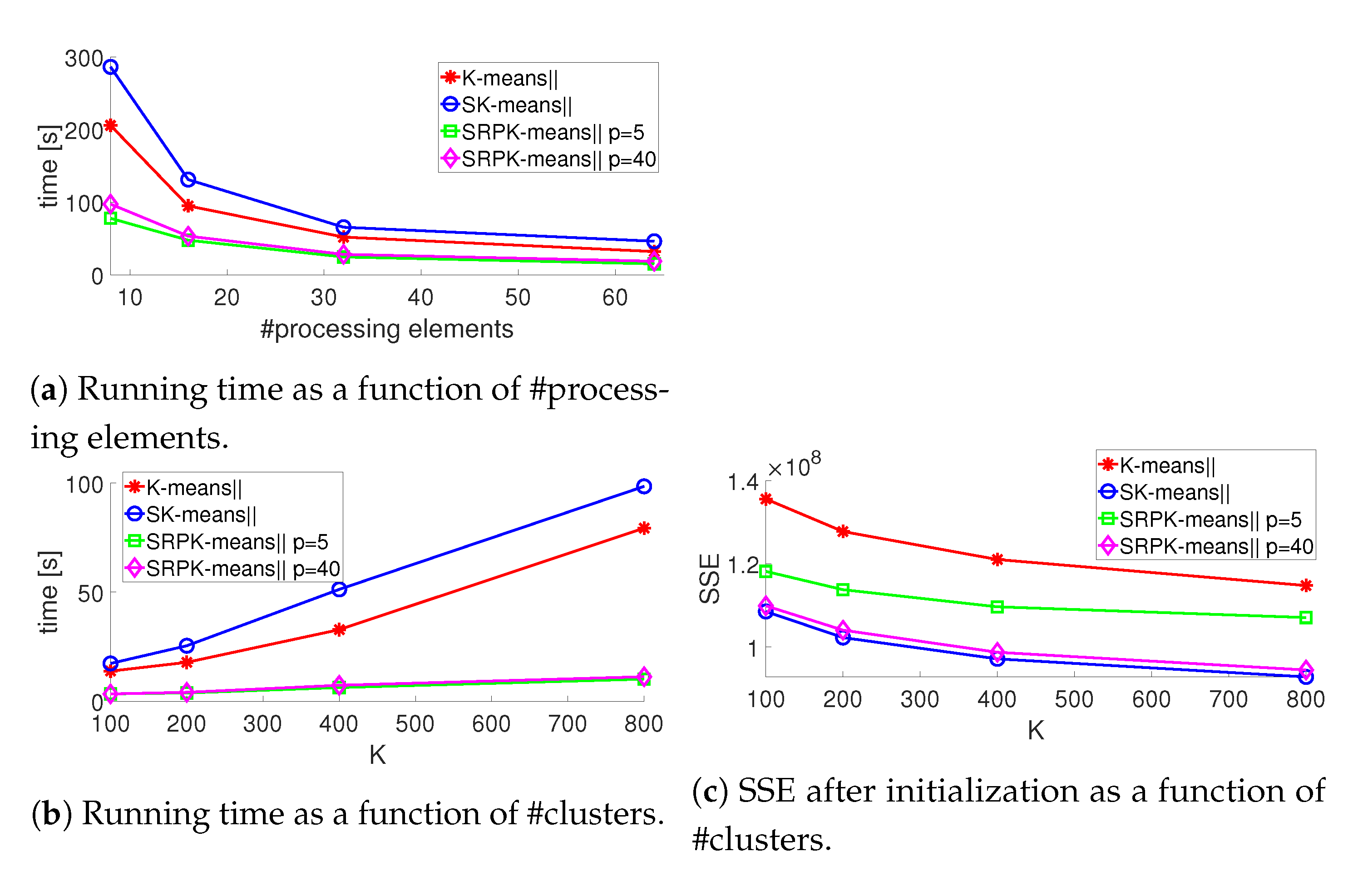
We conducted scalability tests for TIN and SVH to show how running time varies as a function of #processing elements (Matlab workers) and to demonstrate the benefits of using SRPK-means‖ for a very high-dimensional dataset (SVH) when K is increased. We concentrated on the running time of the initialization and the corresponding SSE. We performed scalability experiments in two parts: $\left(1\right)$ Tests with TIN: #processing elements was varied from 8 to 64 and $K=100$ was fixed; $\left(2\right)$ Tests with SVH: The number of clusters was varied as $K\in \{100,200,400,800\}$ and #processing elements was fixed to 32. Otherwise, we used the same parameter settings as in the previous experiments.

Median running time and SSE curves out of 10 runs are shown in Figure 1. Results for the experiment 1 are shown in Figure 1a. In terms of Amdahl’s law [51], K-means‖ and SK-means‖ perform equally well: running time is nearly halved when #processing elements is doubled from 8 to 16 and from 16 to 32. From this perspective, performance of SRPK-means‖ is slightly worse than K-means‖ and SK-means‖. The results for the experiment 2 are shown in Figure 1b,c. Clearly, for very high-dimensional data, SRPK-means‖ runs much faster compared to K-means‖ and SK-means‖. As analyzed in Section 3.2, the speedup for SRPK-means‖ is increased when K is increased. A similar observation was made between K-means++ and RPK-means++ in [28]. Furthermore, when $K=800$, the speedup for SRPK-means‖ with respect to K-means‖ is 7–8 and with respect to SK-means‖ 9–10. Moreover, according to Figure 1c, SRPK-means‖ (when $p=40$) and SK-means‖ sustain their accuracy when K is increased in a frame of K-means‖.

4.2. Experiments with High-Dimensional Synthetic Datasets

Finally, to strengthen the evaluation, we next summarize experiments with novel synthetic datasets, where symmetric, spherical clusters are hidden in a very high-dimensional space. Comparison of K-means initialization methods for datasets with assured spherical shape is clearly relevant because K-means restores such geometries during the clustering process [4,6,44]. Please note that using SSE for high-dimensional data can be ambiguous [52]. As we will next demonstrate, the SSE error difference of good and bad clustering results in a high-dimensional space can be surprisingly small. To show this, we also analyze the final clustering accuracy with normalized mutual information (NMI) [53] with the actual entropies. Please note that it would have been uninformative to use NMI as a quality measure for datasets in Section 4.1 because there we had no information on the cluster geometry. Mutual Information (MI) can be defined as

$$\mathrm{MI}(\mathbf{I},\mathbf{L})=\sum _{k=1}^K\sum _{i=1}^{K^{*}}\frac{n_k^{\left(i\right)}}{n}{log}_2\frac{\frac{n_k^{\left(i\right)}}{n}}{\frac{n^{\left(i\right)}}{n}\frac{n_k}{n}},$$

(2)

where $\mathbf{I}$ refers to the cluster labels, $\mathbf{L}$ to the ground truth labels, $K^{*}$ to the number of unique ground truth labels, and n denotes labels’ frequency counts. Then, NMI can be defined as

$$\mathrm{NMI}(\mathbf{I},\mathbf{L})=\frac{2\mathrm{MI}(\mathbf{I},\mathbf{L})}{H\left(\mathbf{I}\right)+H\left(\mathbf{L}\right)},$$

(3)

where $H\left(\mathbf{I}\right)={log}_2\left(K\right)$ and $H\left(\mathbf{L}\right)={log}_2\left(K^{*}\right)$ denote the entropies of the cluster labels and ground truth labels.

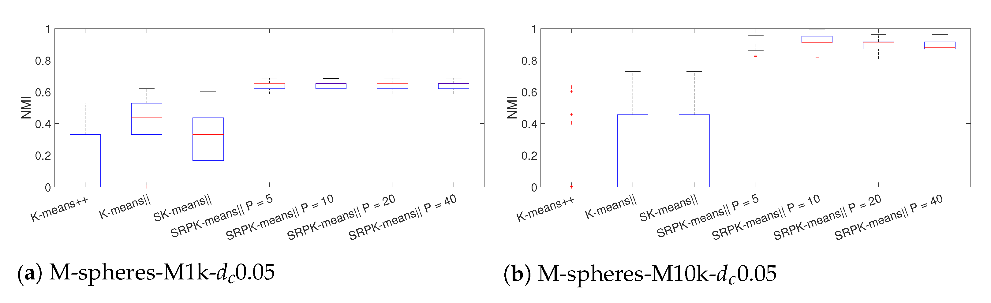
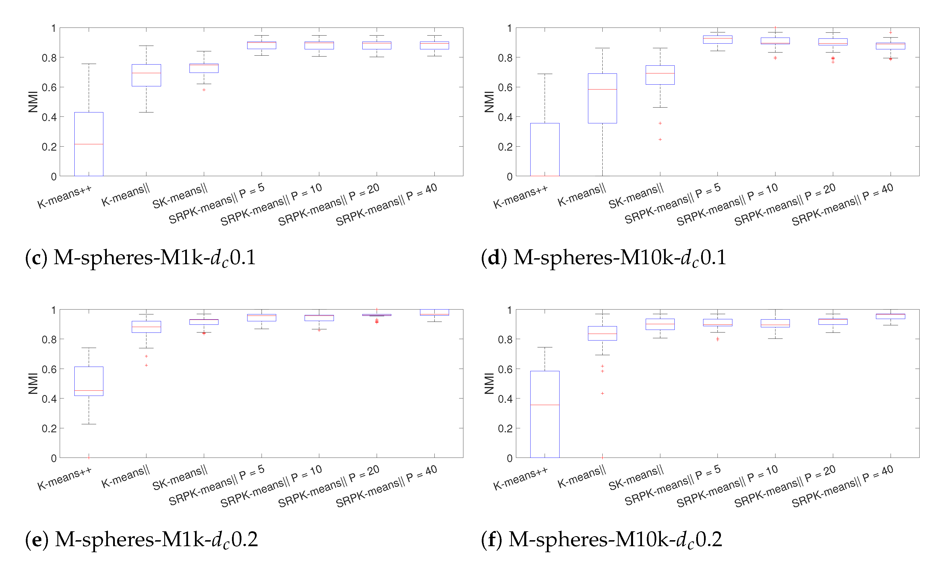
Details of the six generated datasets with Algorithm 4 are summarized in

Table 5. Characteristics of the synthetic datasets.

Dataset	#Observations (N)	#Features (M)	#Clusters (K)	Center Distance (${\mathit{d}}_{\mathit{c}}$)	Radius (${\mathit{d}}_{\mathit{r}}$)
M-spheres-M1k-$d_c$0.05	100,000	1000	10	0.05	1.0
M-spheres-M1k-$d_c$0.1	100,000	1000	10	0.1	1.0
M-spheres-M1k-$d_c$0.2	100,000	1000	10	0.2	1.0
M-spheres-M10k-$d_c$0.05	100,000	10,000	10	0.05	1.0
M-spheres-M10k-$d_c$0.1	100,000	10,000	10	0.1	1.0
M-spheres-M10k-$d_c$0.2	100,000	10,000	10	0.2	1.0

. The generated datasets are referred as M-spheres. For each dataset, we set $N_K=\mathrm{10,000}$, $K=10$, and $d_r=1$. To demonstrate interesting effects in the clustering initialization, we varied the nearest cluster center distance as $d_c=\{0.05,0.1,0.2\}$ and the data dimension as $M=\{1000,\mathrm{10,000}\}$. We set $d_c$ values to much smaller than $d_r$ in order to increase the difficulty of the clustering problems. In Figure 2, PCA projections on the three largest principal components show that the clusters are more separated for $M=\mathrm{10,000}$ than for $M=1000$. For the M-spheres datasets, we used the serial implementations of the initialization methods with the same settings as before.

Results for the final clustering accuracy using NMI with 100 repeats are shown in Figure 3. Clearly, SRPK-means‖ outperforms other methods in terms final clustering accuracy for all the synthetic datasets. Moreover, if we compare the results between the datasets with $M=1000$ and $M=\mathrm{10,000}$, we observe that the clustering accuracy for SRPK-means‖ is improved when the dimensionality increases. The most significant difference is obtained for the M-spheres-M10k-$d_c$0.05 dataset, where K-means++ has a total breakdown of the accuracy while SRPK-means‖ is able find the near optimal clustering result out of 100 repeats. Moreover, the accuracy of K-means++ is clearly worse compared to K-means‖ and SK-means‖ for very high-dimensional datasets. We tested K-means with random initialization for this dataset and observed from the statistical testing that K-means++, K-means‖ and SK-means‖ are no better than the random initialization in terms of NMI. These results demonstrate that the use of distances in the K-means++ type of initialization strategies can become meaningless in very high-dimensional spaces.

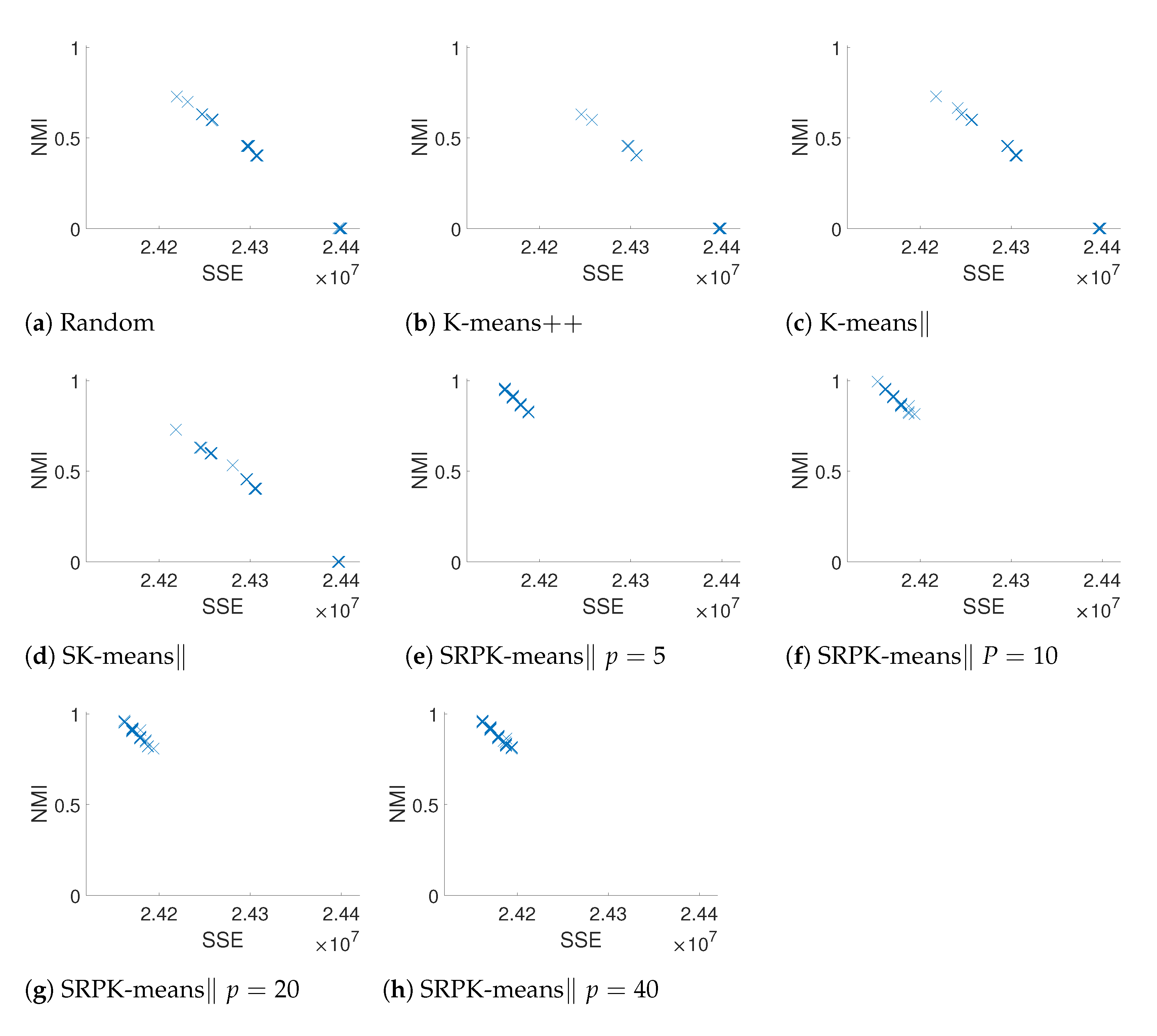
In Figure 4, scatter plots of SSE and NMI values show that the relative SSE difference between worst possible clustering result ($\mathrm{NMI}=0$) and the optimal clustering result ($\mathrm{NMI}=1$) can be surprisingly small for very high-dimensional data. Therefore, the improvements for the final clustering accuracy in Table 2 can be much more significant than the impression given by SSE in terms of how spherical clusters are found for high-dimensional datasets.

Figure 3 and Figure 4 illustrate the deteriorating behavior of the currently most popular K-means++ initialization method in high dimensions. We especially observe that the K-means++ initialization behaves like (i.e., is not better than) the random one in the very high-dimensional cases. Such finding also suggests further experiments, where as a function of the data dimension, emergence of such a behavior is being studied to identify most appropriate random project dimensions to restore the quality of initialization and the whole clustering algorithm.

5. Conclusions

In this paper, we proposed two parallel initialization methods for large-scale K-means clustering and a new high-dimensional clustering data generation algorithm to support their empirical evaluation. The methods are based on divide-and-conquer type of K-means‖ approach and random projections. The proposed initialization methods are scalable and fairly easy to implement with different parallel programming models.

The experimental results for an extensive set of benchmark and novel synthetic datasets showed that the proposed methods improve clustering accuracy and the speed of convergence compared to state-of-the-art approaches. Moreover, the deteriorating behavior of the K-means++ and K-means‖ initialization methods in high dimensions can be recovered with the proposed RP-based approach to provide accurate initialization also for high-dimensional data. Our experiments also confirmed the finding (e.g., [52]) that the difference between the errors (SSE) of good and bad clustering results in high-dimensional spaces can be surprisingly small also challenge cluster validation and cluster validation indices (see [4] and references therein) in such cases.

Experiments with SRPK-means‖ method demonstrate that use of RP and K-means‖ is beneficial for clustering large-scale high-dimensional datasets. In particular, SRPK-means‖ is an appealing approach as a standalone algorithm for clustering very high-dimensional large-scale datasets. In future work, it would be interesting to test a RP-based local SSE selection for SRPK-means‖, which uses the same RP matrix in each subset for the initial prototype selection. In this case, use of sparse RP variants [54] or the mailman algorithm [17] for the matrix multiplication could be beneficial, particularly in applications where K is close to P. Furthermore, integrating the proposed methods into the robust K-means‖ [37] would be beneficial for clustering noisy data, because the clustering problems in these cases are especially challenging.

References

- Lloyd, S. Least squares quantization in PCM. IEEE Trans. Inf. Theory 1982, 28, 129–137. [Google Scholar] [CrossRef]
- Emre Celebi, M.; Kingravi, H.A.; Vela, P.A. A comparative study of efficient initialization methods for the k-means clustering algorithm. Expert Syst. Appl. 2012, 40, 200–210. [Google Scholar] [CrossRef] [Green Version]
- Fränti, P.; Sieranoja, S. How much can k-means be improved by using better initialization and repeats? Pattern Recognit. 2019, 93, 95–112. [Google Scholar] [CrossRef]
- Hämäläinen, J.; Jauhiainen, S.; Kärkkäinen, T. Comparison of Internal Clustering Validation Indices for Prototype-Based Clustering. Algorithms 2017, 10, 105. [Google Scholar] [CrossRef] [Green Version]
- Arthur, D.; Vassilvitskii, S. k-means++: The advantages of careful seeding. In Proceedings of the Eighteenth Annual ACM-SIAM Symposium on Discrete Algorithms, Society for Industrial and Applied Mathematics, New Orleans, LA, USA, 7–9 January 2007; pp. 1027–1035. [Google Scholar]
- Bahmani, B.; Moseley, B.; Vattani, A.; Kumar, R.; Vassilvitskii, S. Scalable K-means++. Proc. VLDB Endow. 2012, 5, 622–633. [Google Scholar] [CrossRef]
- Xu, Y.; Qu, W.; Li, Z.; Min, G.; Li, K.; Liu, Z. Efficient k -Means++ Approximation with MapReduce. IEEE Trans. Paral. Distrib. Syst. 2014, 25, 3135–3144. [Google Scholar] [CrossRef] [Green Version]
- Dhillon, I.S.; Modha, D.S. A data-clustering algorithm on distributed memory multiprocessors. In Large-Scale Parallel Data Mining; Springer: New York, NY, USA, 2002; pp. 245–260. [Google Scholar]
- Zhao, W.; Ma, H.; He, Q. Parallel K-Means Clustering Based on MapReduce. In Proceedings of the 1st International Conference on Cloud Computing, CloudCom ’09, Munich, Germany, 19–21 October 2009; pp. 674–679. [Google Scholar]
- Elkan, C. Using the triangle inequality to accelerate k-means. In Proceedings of the 20th International Conference on Machine Learning (ICML-03), Washington, DC, USA, 21–24 August 2003; pp. 147–153. [Google Scholar]
- Hamerly, G. Making k-means even faster. In Proceedings of the 2010 SIAM International Conference on Data Mining, Columbus, OH, USA, 29 April–1 May 2010; pp. 130–140. [Google Scholar]
- Drake, J.; Hamerly, G. Accelerated k-means with adaptive distance bounds. In Proceedings of the 5th NIPS Workshop On Optimization for Machine Learning, Lake Tahoe, NV, USA, 7–8 December 2012; pp. 42–53. [Google Scholar]
- Ding, Y.; Zhao, Y.; Shen, X.; Musuvathi, M.; Mytkowicz, T. Yinyang k-means: A drop-in replacement of the classic k-means with consistent speedup. Int. Conf. Mach. Learn. 2015, 37, 579–587. [Google Scholar]
- Bottesch, T.; Bühler, T.; Kächele, M. Speeding up k-means by approximating Euclidean distances via block vectors. Int. Conf. Mach. Learn. 2016, 2578–2586. Available online: http://proceedings.mlr.press/v48/bottesch16.pdf (accessed on 24 December 2020).
- Bachem, O.; Lucic, M.; Lattanzi, S. One-shot coresets: The case of k-clustering. In International Conference On Artificial Intelligence And Statistics; PMLR: Canary Islands, Spain, 2018; pp. 784–792. [Google Scholar]
- Capó, M.; Pérez, A.; Lozano, J.A. An efficient K-means clustering algorithm for massive data. arXiv 2018, arXiv:1801.02949. [Google Scholar]
- Boutsidis, C.; Zouzias, A.; Drineas, P. Random projections for k-means clustering. Adv. Neural Inf. Process. Syst. 2010, 23, 298–306. [Google Scholar]
- Fern, X.; Brodley, C. Random projection for high dimensional data clustering: A cluster ensemble approach. In Proceedings of the 20th International Conference on Machine Learning, Washington, DC, USA, 21–24 August 2003; pp. 186–193. [Google Scholar]
- Alzate, C.; Suykens, J.A. Multiway spectral clustering with out-of-sample extensions through weighted kernel PCA. IEEE Trans. Pattern Anal. Mach. Intell. 2010, 32, 335–347. [Google Scholar] [CrossRef]
- Napoleon, D.; Pavalakodi, S. A new method for dimensionality reduction using K-means clustering algorithm for high dimensional data set. Int. J. Comput. Appl. 2011, 13, 41–46. [Google Scholar]
- Liu, H.; Motoda, H. Feature Selection for Knowledge Discovery and Data Mining; Kluwer Academic Publishers: Norwell, MA, USA, 1998. [Google Scholar]
- Achlioptas, D. Database-friendly random projections: Johnson-Lindenstrauss with binary coins. J. Comput. Syst. Sci. 2003, 66, 671–687, Special Issue on {PODS} 2001. [Google Scholar] [CrossRef] [Green Version]
- Jolliffe, I.T. Principal Component Analysis; Springer: New York, NY, USA, 2002. [Google Scholar]
- Bingham, E.; Mannila, H. Random Projection in Dimensionality Reduction: Applications to Image and Text Data. In Proceedings of the Seventh ACM SIGKDD International Conference on Knowledge Discovery and Data Mining, San Francisco, CA, USA, 26–29 August 2001; pp. 245–250. [Google Scholar]
- Cohen, M.B.; Elder, S.; Musco, C.; Musco, C.; Persu, M. Dimensionality reduction for k-means clustering and low rank approximation. In Proceedings of the Forty-Seventh Annual ACM Symposium on Theory of Computing, Portland, OR, USA, 15–17 June 2015; pp. 163–172. [Google Scholar]
- Boutsidis, C.; Zouzias, A.; Mahoney, M.W.; Drineas, P. Randomized dimensionality reduction for k-means clustering. IEEE Trans. Inf. Theory 2014, 61, 1045–1062. [Google Scholar] [CrossRef] [Green Version]
- Cardoso, Â.; Wichert, A. Iterative random projections for high-dimensional data clustering. Pattern Recognit. Lett. 2012, 33, 1749–1755. [Google Scholar] [CrossRef]
- Chan, J.Y.; Leung, A.P. Efficient k-means++ with random projection. In Proceedings of the 2017 International Joint Conference on Neural Networks (IJCNN), IEEE, Anchorage, AK, USA, 14–19 May 2017; pp. 94–100. [Google Scholar]
- Sarkar, S.; Ghosh, A.K. On perfect clustering of high dimension, low sample size data. IEEE Trans. Pattern Anal. Mach. Intell. 2019. Available online: https://www.isical.ac.in/~statmath/report/74969-cluster.pdf (accessed on 24 December 2020).
- Hämäläinen, J.; Kärkkäinen, T. Initialization of Big Data Clustering using Distributionally Balanced Folding. In Proceedings of the European Symposium on Artificial Neural Networks, Computational Intelligence and Machine Learning-ESANN 2016, Bruges, Belgium, 27–29 April 2016; pp. 587–592. [Google Scholar]
- Moreno-Torres, J.G.; Sáez, J.A.; Herrera, F. Study on the Impact of Partition-Induced Dataset Shift on k-fold Cross-Validation. IEEE Trans. Neural Netw. Learn. Syst. 2012, 23, 1304–1312. [Google Scholar] [CrossRef] [PubMed]
- Vattani, A. K-means requires exponentially many iterations even in the plane. Discr. Comput. Geom. 2011, 45, 596–616. [Google Scholar] [CrossRef] [Green Version]
- MacQueen, J. Some methods for classification and analysis of multivariate observations. In Proceedings of the Fifth Berkeley Symposium on Mathematical Statistics and Probability; University of California Press: Berkeley, CA, USA, 1967; Volume 1, pp. 281–297. Available online: https://stacks.stanford.edu/file/druid:xb208zr6261/xb208zr6261.pdf (accessed on 24 December 2020).
- Forgy, E.W. Cluster analysis of multivariate data: Efficiency vs. interpretability of classifications. Biometrics 1965, 21, 768–769. [Google Scholar]
- Bradley, P.S.; Fayyad, U.M. Refining Initial Points for K-Means Clustering. ICML 1998, 98, 91–99. [Google Scholar]
- Bachem, O.; Lucic, M.; Krause, A. Distributed and provably good seedings for k-means in constant rounds. Int. Conf. Mach. Learn. 2017, 70, 292–300. [Google Scholar]
- Hämäläinen, J.; Kärkkäinen, T.; Rossi, T. Scalable robust clustering method for large and sparse data. In Proceedings of the European Symposium on Artificial Neural Networks, Computational Intelligence and Machine Learning-ESANN 2018, Bruges, Belgium, 25–27 April 2018; pp. 449–454. [Google Scholar]
- Johnson, W.B.; Lindenstrauss, J. Extensions of Lipschitz mappings into a Hilbert space. Contemp. Math. 1984, 26, 1. [Google Scholar]
- Rezaei, M.; Fränti, P. Can the Number of Clusters Be Determined by External Indices? IEEE Access 2020, 8, 89239–89257. [Google Scholar] [CrossRef]
- Bottou, L.; Bengio, Y. Convergence properties of the k-means algorithms. Adv. Neural Inf. Process. Syst. 1995, 585–592. Available online: https://papers.nips.cc/paper/1994/file/a1140a3d0df1c81e24ae954d935e8926-Paper.pdf (accessed on 24 December 2020).
- Broder, A.; Garcia-Pueyo, L.; Josifovski, V.; Vassilvitskii, S.; Venkatesan, S. Scalable k-means by ranked retrieval. In Proceedings of the 7th ACM International Conference on Web Search and Data Mining, New York, NY, USA, 24–28 February 2014; pp. 233–242. [Google Scholar]
- Sharma, G.; Martin, J. MATLAB®: A Language for Parallel Computing. Int. J. Parallel Progr. 2009, 37, 3–36. [Google Scholar] [CrossRef] [Green Version]
- Muller, M.E. Some continuous Monte Carlo methods for the Dirichlet problem. Ann. Math. Stat. 1956, 27, 569–589. [Google Scholar] [CrossRef]
- Fränti, P.; Sieranoja, S. K-means properties on six clustering benchmark datasets. Appl. Intell. 2018, 48, 1–17. [Google Scholar] [CrossRef]
- De Vries, C.M.; Geva, S. K-tree: Large scale document clustering. In Proceedings of the 32nd International ACM SIGIR Conference on Research and Development in Information Retrieval, Boston, MA, USA, 19–23 July 2009; pp. 718–719. [Google Scholar]
- Kriegel, H.P.; Schubert, E.; Zimek, A. The (black) art of runtime evaluation: Are we comparing algorithms or implementations? Knowl. Inf. Syst. 2017, 52, 341–378. [Google Scholar] [CrossRef]
- Gallego, A.J.; Calvo-Zaragoza, J.; Valero-Mas, J.J.; Rico-Juan, J.R. Clustering-based k-nearest neighbor classification for large-scale data with neural codes representation. Pattern Recognit. 2018, 74, 531–543. [Google Scholar] [CrossRef] [Green Version]
- Kruskal, W.H.; Wallis, W.A. Use of ranks in one-criterion variance analysis. J. Am. Stat. Assoc. 1952, 47, 583–621. [Google Scholar] [CrossRef]
- Saarela, M.; Hämäläinen, J.; Kärkkäinen, T. Feature Ranking of Large, Robust, and Weighted Clustering Result. In Proceedings of the 21st Pacific Asia Conference on Knowledge Discovery and Data Mining-PAKDD 2017, Jeju, Korea, 23–26 May 2017; pp. 96–109. [Google Scholar]
- Äyrämö, S. Knowledge Mining Using Robust Clustering; Vol. 63 of Jyväskylä Studies in Computing; University of Jyväskylä: Jyväskylä, Finland, 2006. [Google Scholar]
- Amdahl, G.M. Validity of the single processor approach to achieving large scale computing capabilities. AFIPS Conf. Proc. 1967, 30, 483–485. [Google Scholar]
- Aggarwal, C.C.; Hinneburg, A.; Keim, D.A. On the surprising behavior of distance metrics in high dimensional space. In International Conference On Database Theory; Springer: New York, NY, USA, 2001; pp. 420–434. [Google Scholar]
- Strehl, A. Relationship-Based Clustering and Cluster Ensembles for High-Dimensional Data Mining. Ph.D. Thesis, The University of Texas at Austin, Austin, TX, USA, 2002. [Google Scholar]
- Li, P.; Hastie, T.J.; Church, K.W. Very sparse random projections. In Proceedings of the 12th ACM SIGKDD International Conference on Knowledge diScovery and Data Mining, Philadelphia, PA, USA, 20–23 August 2006; pp. 287–296. [Google Scholar]
Figure 1.
Scalability.
Figure 2.
Synthetic dataset projections on the three largest principal components.
Figure 3.
NMI for the synthetic datasets.
Figure 4.
Scatter plot of SSE and NMI results for the M-spheres-M10k-0.05 dataset.